Spatiotemporal analysis of phenological metrics on the Qinghai-Tibet Plateau based on multiple vegetation indices

As global climate change intensifies, understanding the response mechanisms and adaptive capacities of ecosystems to climate change has become a core focus in environmental science. The Qinghai-Tibet Plateau (QTP), a region highly sensitive to global climate change, shows vegetation phenological shifts that reflect the ecosystem’s response to climate fluctuations. However, how phenological metrics extracted from different vegetation indices affect our understanding of these shifts in the region remains unclear. This study analyzes the start (SOS) and end (EOS) of the growing season on the QTP from 1982 to 2015 using GIMMS NDVI3g data. These metrics were compared with phenological data derived from GIMMS LAI3g and MODIS EVI2 data. The results indicate that phenological metrics derived from different vegetation indices (NDVI, LAI, and EVI2) are generally consistent in their spatiotemporal distribution and show significant correlations. However, regional differences and temporal inconsistencies were observed. This comparative analysis reveals the strengths and limitations of various vegetation indices in phenological metric extraction. The results offer crucial insights for enhancing the precision of phenological modeling and highlight the significance of choosing suitable vegetation indices in future studies on phenology.

1 Introduction

With the accelerating pace of global climate change, investigating the mechanisms by which ecosystems respond and adapt to these changes has become a central issue in ecological and environmental researches (Cohen et al., 2021; Haddeland et al., 2014). Phenology, as an important branch of study that examines the periodic biological activities of organisms (such as plant budding, flowering, and leaf fall) and their relationships with environmental changes, has garnered significant attention in recent years (Hmimina et al., 2013; Liu et al., 2020). Phenological metrics not only reflect vegetation responses to climate change but also serve as indicators of ecosystem health. Therefore, accurately extracting and analyzing these metrics is of critical importance in global change research (Bolton et al., 2020; Chen et al., 2019; Liu et al., 2017).

In this context, the Qinghai-Tibet Plateau (QTP), known for its sensitivity to global climate change, has emerged as a key region for phenological research (Shen et al., 2011; Zheng et al., 2016). The region’s unique geographic environment and climatic conditions make its vegetation phenological changes particularly responsive to climate fluctuations. Examining these phenological shifts can uncover the influence of climate change on the region’s growing season, ecosystem functions, and carbon cycles, offering greater insight into the ecological consequences of climate change (Ding et al., 2016; Zhang et al., 2013).

Remote sensing has emerged as a powerful tool in phenological studies, enabling large-scale and continuous monitoring of vegetation dynamics in complex environments such as mountainous regions (Orusa et al., 2020)​. Satellite-based platforms like MODIS, Sentinel-2, and Landsat have been instrumental in extracting key phenological metrics like the start of growing season (SOS), end of growing season (EOS), and length of growing season (LOS), contributing to our understanding of vegetation responses to climate variations across different altitudes (Orusa et al., 2023a; Orusa and Borgogno Mondino, 2021; Viani et al., 2023)​. The application of remote sensing in mountainous regions, such as the QTP, provides valuable data for assessing vegetation patterns under the stress of changing climatic conditions (Orusa et al., 2023b; Viani et al., 2024)​. Studies have also shown that these techniques are essential for developing ecological services aimed at monitoring and mitigating the impacts of climate change on high-altitude ecosystems (Orusa et al., 2020; Orusa et al., 2024; Viani et al., 2024)​.

Vegetation indices like the Normalized Difference Vegetation Index (NDVI) and Enhanced Vegetation Index (EVI) have been widely used to capture phenological patterns (Jiang et al., 2008; Yang et al., 2022). In recent years, the extraction of phenological metrics from remote sensing data has advanced significantly, with various vegetation indices demonstrating distinct strengths and limitations in this process (Wu et al., 2021; Zeng et al., 2013; Zhang et al., 2003). Researchers have extensively utilized these vegetation indices to extract phenological metrics and have explored their performance in capturing seasonal dynamics of vegetation growth (Piao et al., 2011). Among these indices, NDVI, being one of the earliest and most commonly used, is particularly sensitive to green vegetation and is widely acknowledged for its effectiveness in capturing seasonal variations in vegetation growth (Høgda et al., 2013; Zhang J. et al., 2020). Studies have shown that NDVI-based phenological extraction methods perform well in large-scale, long-term studies, but NDVI tends to saturate in areas with high vegetation coverage and is sensitive to atmospheric effects (Jiang et al., 2008). To address these limitations, EVI was introduced. EVI accounts for atmospheric scattering and soil background noise, allowing for more accurate reflection of phenological changes in areas with high vegetation coverage (Zhang et al., 2003). Research has found that EVI-based phenological metrics perform exceptionally well in high-coverage regions such as tropical rainforests, providing more accurate phenological information than NDVI (Ganguly et al., 2010). Moreover, other vegetation indices like the Wide Dynamic Range Vegetation Index (WDRVI) and the Greenness Chromatic Coordinate (GCC) have demonstrated particular advantages in phenological extraction for certain ecosystems and vegetation types (Gitelson, 2004; Richardson et al., 2018). Studies have demonstrated that remote sensing data, particularly when processed through platforms like Google Earth Engine, can significantly enhance the mapping of phenological metrics in mountain areas, providing a robust framework for global monitoring (Orusa et al., 2020; Orusa et al., 2023a; Orusa et al., 2023b)​.

However, despite these advances, challenges remain in accurately capturing phenological patterns in high-altitude environments like the QTP. Factors such as cloud cover, terrain complexity, and sparse ground validation data can introduce uncertainties (Zhang J. et al., 2020). There is a need for further validation and comparison of different vegetation indices to assess their performance in capturing phenological metrics across diverse temporal and spatial scales.

Therefore, this study seeks to thoroughly analyze the similarities and differences in phenological metrics derived from various vegetation indices within the QTP. The major objectives of the study are: (a) to compare the performance of different vegetation indices (NDVI, EVI, GCC, etc.) in capturing phenological metrics across different ecosystems in the QTP; (b) to assess the strengths and limitations of these indices in characterizing phenological trends in response to climate change; (c) to provide insights into how ecosystems in the QTP respond to climate fluctuations, using long-term remote sensing data. Through this analysis, the study will offer a scientific foundation for phenological research in the context of global change, enriching our understanding of ecosystem responses to climate change.

2 Study area and dataset

2.1 Study area

The QTP (Figure 1) stands as the world’s largest and highest plateau. The QTP, with its distinct natural geography and ecosystems, is a vital water source conservation area for Asia, where rivers originating from this region influence the lives and livelihoods of hundreds of millions in surrounding areas. The QTP’s high elevation and unique climatic conditions make its ecosystems highly sensitive to climate change and human activities. Consequently, the plateau is regarded as one of the frontiers and hotspots for global climate change research (Ganjurjav et al., 2020).

Figure 1

Figure 1. Study area.

2.2 NDVI data

The third-generation Global Inventory Modeling and Mapping Studies Normalized Difference Vegetation Index product (GIMMS NDVI3g), developed based on AVHRR sensor data, is currently the longest-running global NDVI time series product available. GIMMS NDVI3g has undergone extensive preprocessing, including radiometric calibration, coordinate transformation, geometric correction, and atmospheric correction, while also eliminating the effects of orbital drift caused by solar zenith angle (Pinzón et al., 2005), differences between the second- and third-generation AVHRR sensors (Anyamba et al., 2014), and the adverse impacts of stratospheric aerosols and cloud cover during events such as El Niño and the Mount Pinatubo eruption. Compared to its predecessor, NDVI3g has improved snowmelt calibration detection algorithms and resolved data discontinuities in high-latitude areas of the Northern Hemisphere (Zhu et al., 2013). GIMMS NDVI3g delivers global NDVI data covering the period from July 1981 to December 2015, featuring a 1/12° spatial resolution and a 15-day temporal resolution.

2.3 Land surface phenology

We utilized two existing land surface phenology data products. The first dataset is the MODIS Global Land Surface Phenology product (MCD12Q2), based on EVI2 time series, with a 500-m spatial resolution and coverage from 2001 to 2018. The second dataset is derived from the GIMMS LAI3g time series (LAI_PhenoData), providing global land surface phenology data (Wu and Xin, 2022). This dataset features two primary phenological metrics, SOS and EOS, covering the years 1982–2015 at a 1/12° spatial resolution.

2.4 Other data

We also employed the MODIS Global Land Cover Type product (MCD12Q1), which features a 500-m spatial resolution and an annual temporal resolution. Among its five classification schemes, we chose the International Geosphere-Biosphere Programme (IGBP) scheme to identify vegetation-covered areas on the QTP for subsequent phenological analysis.

3 Methodology

To assess and compare the similarities and distinctions in phenological metrics obtained from multiple vegetation indices, we first selected the Greenup and Dormancy bands from the MCD12Q2 phenology product, based on EVI2, to represent SOS and EOS in the vegetation growth process, respectively. Next, we derived the phenological metrics (i.e., SOS and EOS) for the growing season of the QTP from the LAI_PhenoData (Wu and Xin, 2022). Finally, we extracted the annual SOS and EOS for the QTP from 1982 to 2015 using GIMMS NDVI3g time series data, as detailed below (Figure 2).

Figure 2

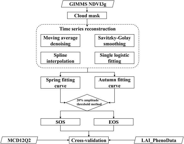
Figure 2. Flowchart of phenology retrieval.

3.1 Data pre-processing

Using the quality control band of the GIMMS NDVI3g product, we excluded pixels severely affected by clouds, aerosols, and other disturbances. During the data pre-processing stage, we identified points exceeding three times the standard deviation of the moving window median (with a window length of 7 points) as invalid outliers. The Savitzky-Golay filter (Savitzky and Golay, 1964) was applied to smooth the NDVI time series. Additionally, we used spline interpolation to resample the NDVI data to a daily scale.

3.2 Time series fitting

In this study, we employed a single logistic curve fitting function to segmentally model the spring growth phase (i.e., the continuous rise in the NDVI time series from a local minimum to a local maximum) and the autumn senescence phase (i.e., the continuous decline in the NDVI time series from a local maximum to a local minimum) during the vegetation growth cycle (Zhang et al., 2003). The underlying principle is as follows (Equations 1, 2):

${\mathit{N}\mathit{D}\mathit{V}\mathit{I}}_{\mathit{s}\mathit{p}\mathit{r}\mathit{i}\mathit{n}\mathit{g}}\left(\mathit{t}\right)=\frac{\mathit{a}\mathit{m}\mathit{p}}{\mathbf{1}+{\mathbf{e}}^{\mathit{a}+\mathit{b}*\mathit{t}}}+\mathit{m}\mathit{i}\mathit{n}\mathit{v}(1)$

${\mathit{N}\mathit{D}\mathit{V}\mathit{I}}_{\mathit{a}\mathit{u}\mathit{t}\mathit{u}\mathit{m}\mathit{n}}\left(\mathit{t}\right)=-\frac{\mathit{a}\mathit{m}\mathit{p}}{\mathbf{1}+{\mathbf{e}}^{\mathit{a}+\mathit{b}*\mathit{t}}}+\mathit{m}\mathit{a}\mathit{x}\mathit{v}(2)$

${NDVI}_{spring}$ represents the NDVI value during the spring growth phase of vegetation, and ${NDVI}_{autumn}$ represents the NDVI value during the autumn senescence phase. The variable t denotes the day of the year, a and b are fitting parameters, amp is the amplitude of the NDVI time series, minv is the minimum value, and maxv is the maximum value of the NDVI time series.

3.3 Retrieval of phenology metrics

The dynamic threshold method sets thresholds derived from the seasonal amplitude in the vegetation index time series to extract key phenological metrics (Fischer, 1994; Jönsson and Eklundh, 2004). Here, we used 20% of the NDVI amplitude as the threshold to extract SOS and EOS. Specifically, SOS is identified as the point when NDVI initially rises above this threshold in the spring, while EOS is marked by the point when NDVI falls below this threshold for the last time in the autumn.

It is important to note that the time span for the phenological metrics extracted from NDVI and the phenology dataset derived from LAI both cover the period from 1982 to 2015. Therefore, to facilitate comparative analysis, we also limited the MCD12Q2 phenology data to the period from 2001 to 2015.

3.4 Trend analysis and statistical testing

To assess the temporal trends of phenological metrics (i.e., SOS and EOS) during the study period, we applied the Mann-Kendall (MK) trend test. The MK test was conducted on the SOS and EOS extracted from various vegetation indices (i.e., NDVI, LAI, EVI2) to detect significant trends. The slope produced by the MK test was used to quantify the magnitude of the trend, representing the rate of change per year (days/year). We set the significance level at a p-value threshold of 0.05; if the p-value was less than 0.05, the trend was considered significant. Additionally, none of the time series data were detrended prior to trend analysis to ensure the capture of long-term climate change effects on phenological changes.

Note that all data processing in this study was performed using MATLAB R2020a.

4 Results

4.1 Comparison and validation of phenological metrics

To assess the reliability of the phenological metrics derived from NDVI data in this study, we compared them with metrics obtained from EVI2 (MCD12Q2) and LAI data. Figure 3 illustrates a comparison of SOS for the QTP in 2010, derived from NDVI, LAI, and EVI2 data. In terms of spatial distribution, the three datasets exhibit similar patterns, with SOS generally advancing from the northwest to the southeast (Figures 2A–C). However, the SOS derived from LAI is relatively later along the southern edge of the QTP. The NDVI-derived SOS has relatively fewer missing values and tends to be slightly later overall. Figure 3D illustrates the mean changes in SOS along the latitudinal direction, where all three datasets show a trend of SOS initially delaying and then advancing with increasing latitude. The correlation coefficients r between NDVI-derived SOS (N-SOS) and LAI-derived SOS (L-SOS) and EVI2-derived SOS (E-SOS) are 0.841 and 0.864, respectively. Figure 3E presents a scatter density plot comparing N-SOS and L-SOS in terms of spatial distribution, demonstrating a high degree of consistency (R = 0.868, RMSE = 18.85 days). Similarly, Figure 3F shows a scatter density plot comparing N-SOS and E-SOS, which also exhibits strong consistency, with R = 0.890 and RMSE = 16.16 days.

Figure 3

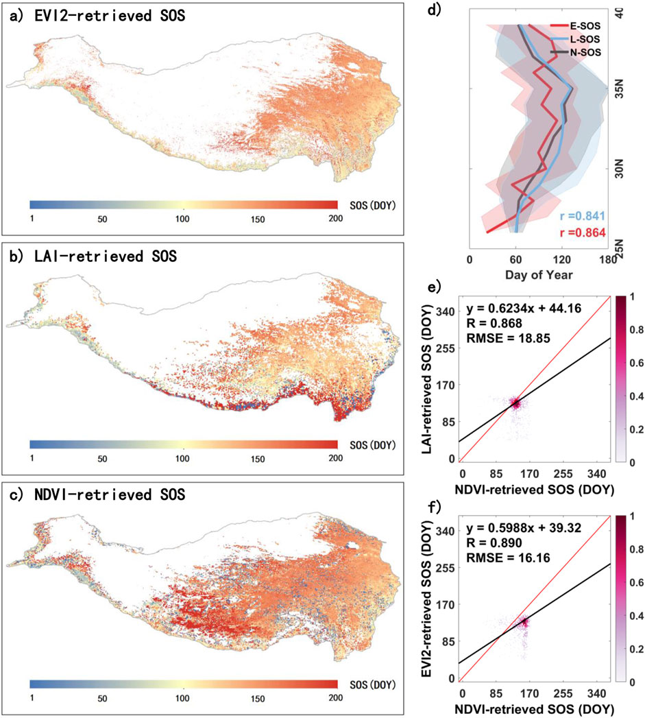
Figure 3. Comparison of SOS on the QTP extracted from multiple vegetation indices for 2010. (A), (B), and (C) represent the EVI2-retrieved SOS (E-SOS), LAI-retrieved SOS (L-SOS), and NDVI-retrieved SOS (N-SOS) on the QTP in 2010, respectively. (D) shows the latitudinal variation of E-SOS, L-SOS, and N-SOS, while (E) and (F) are scatter density plots of N-SOS compared with L-SOS and E-SOS, respectively, in spatial distribution.

Similarly, we compared EOS for the QTP in 2010, as extracted from NDVI, LAI, and EVI2 data (Figure 4). NDVI-derived EOS (N-EOS) and LAI-derived EOS (L-EOS) and EVI2-derived EOS (E-EOS) all exhibit a spatial distribution pattern where timing gradually delays from the northwest to the southeast (Figures 3A–C). However, L-EOS shows a relatively earlier timing along the southern edge of the QTP. N-EOS has relatively fewer missing values overall. In the latitudinal direction, both E-EOS (r = 0.828) and L-EOS (r = 0.844) show a high degree of consistency with N-EOS and display a trend of advancing EOS with increasing latitude (Figure 4D). Figure 4E presents a scatter density plot comparing N-EOS and L-EOS in terms of spatial distribution, demonstrating a high level of consistency (R = 0.851, RMSE = 20.08 days). Similarly, Figure 4F shows a scatter density plot comparing N-EOS and E-EOS, which also exhibits strong consistency, with R = 0.887 and RMSE = 17.32 days.

Figure 4

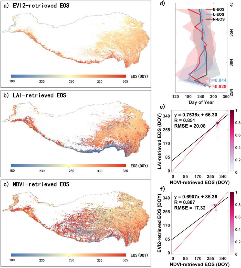
Figure 4. Comparison of EOS on the QTP extracted from multiple vegetation indices for 2010. (A), (B), and (C) represent the EVI2-retrieved EOS (E-EOS), LAI-retrieved EOS (L-EOS), and NDVI-retrieved EOS (N-EOS) on the QTP in 2010, respectively. (D) shows the latitudinal variation of E-EOS, L-EOS, and N-EOS, while (E) and (F) are scatter density plots of N-EOS compared with L-EOS and E-EOS, respectively, in spatial distribution.

4.2 Spatial distributions

To clarify the long-term phenological distribution on the QTP, we calculated the multi-year average results for E-SOS (2001-2015), L-SOS (1982-2015), and N-SOS (1982-2015) (Figure 5). Overall, the spatial distribution of the three is generally consistent, showing a pattern of later SOS in the northwest and earlier SOS in the southeast. However, E-SOS has a higher number of missing values, especially in the central region of the QTP (Figure 5A). L-SOS indicates a comparatively later SOS along the southern edge of the QTP (Figure 5B).

Figure 5

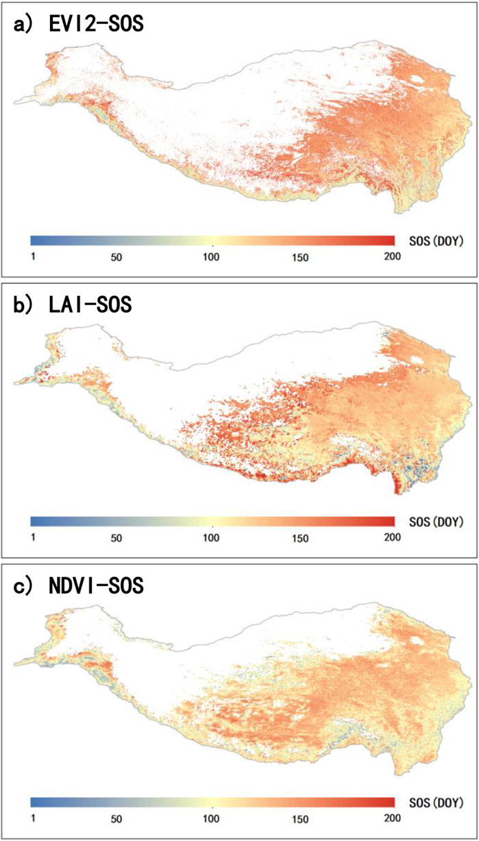
Figure 5. Spatial distribution of the annual mean SOS on the QTP. Panels (A), (B), and (C) represent the mean SOS retrieved from EVI2 (E-SOS) for 2001 to 2015, LAI (L-SOS) for 1982 to 2015, and NDVI (N-SOS) for 1982 to 2015, respectively.

Similarly, we also calculated the multi-year average results for E-EOS (2001-2015), L-EOS (1982-2015), and N-EOS (1982-2015) on the QTP (Figure 6). Overall, E-EOS, L-EOS, and N-EOS all display a spatial pattern of progressively delayed EOS from the northwest to the southeast. However, E-EOS generally occurs relatively earlier and has more missing values (Figure 6A). L-EOS also shows a significant number of missing values (Figure 6B).

Figure 6

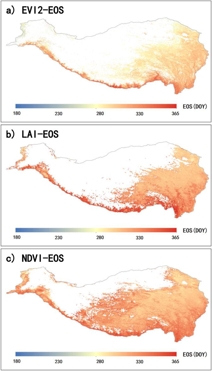
Figure 6. Spatial distribution of the annual mean EOS on the QTP. Panels (A), (B), and (C) represent the mean EOS retrieved from EVI2 (E-EOS) for 2001 to 2015, LAI (L-EOS) for 1982 to 2015, and NDVI (N-EOS) for 1982 to 2015, respectively.

4.3 Trends analysis

We examined the interannual variations of the annual mean SOS and EOS on the QTP (Figure 7). From 1982 to 2015, both N-SOS and L-SOS showed significant delaying trends, with delays of 1.032 days per year (p < 0.01) and 0.171 days per year (p < 0.05), respectively. In contrast, E-SOS advanced at a rate of 0.321 days per year (p < 0.05) from 2001 to 2015 (Figure 7A). Figure 7B depicts the trends for N-EOS, L-EOS, and E-EOS. Notably, N-EOS and L-EOS exhibited opposite trends: from 1982 to 2015, N-EOS delayed significantly by 0.248 days per year (p < 0.05), while L-EOS advanced by 0.107 days per year (p < 0.05). During 2001 to 2015, E-EOS demonstrated a significant delay, with a rate of 0.430 days per year (p < 0.05).

Figure 7

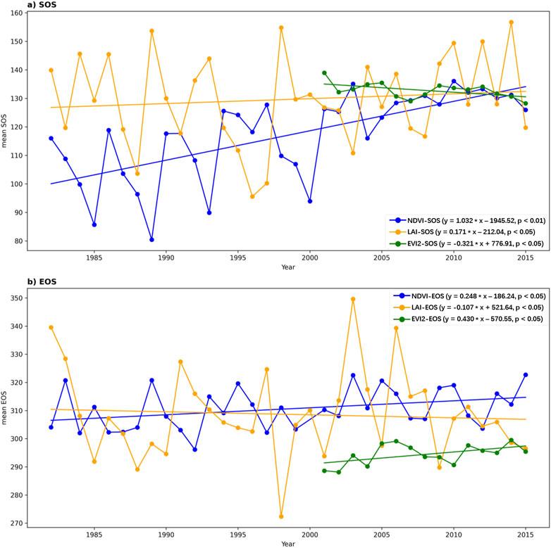
Figure 7. Trends in Annual Mean SOS and EOS on the QTP. (A) illustrates the temporal trends for E-SOS (2001-2015), L-SOS (1982-2015), and N-SOS (1982-2015) on the QTP. (B) illustrates the temporal trends for E-EOS (2001-2015), L-EOS (1982-2015), and N-EOS (1982-2015) on the QTP.

5 Discussion

Most current remote sensing phenology studies rely on a single vegetation index to extract phenological metrics (Ruan et al., 2021; Wu and Wu, 2024; Wu and Xin, 2023). However, there are notable differences in the principles and applications of various vegetation indices (Jiang et al., 2008). To evaluate how different vegetation indices affect phenological extraction, this study conducted a comparative analysis of the spatiotemporal distribution of vegetation phenology metrics on the QTP, utilizing data from various remote sensing vegetation indices. The phenological metrics retrieved from NDVI, LAI, and EVI2 were not entirely consistent in their spatiotemporal distribution. Spatially, the phenological metrics derived from NDVI had fewer missing values, while E-SOS, E-EOS, and L-EOS exhibited noticeably more missing values (Figures 4, 5). There are two potential reasons for this: first, the original vegetation index time series might have poor quality with significant data gaps; second, a complete vegetation growth cycle may span across two consecutive years, leading to failures in fitting the vegetation index time series (Wu et al., 2021). Additionally, among the phenological metrics extracted using the three different vegetation indices, N-SOS was relatively earlier in most areas, while L-SOS tended to be later. Conversely, E-EOS was generally earlier, while N-EOS was relatively later. It is also worth noting that anomalies in SOS and EOS were observed along the southern edge of the QTP when extracted from LAI. Overall, the phenological metrics extracted from different vegetation indices were generally consistent in their spatial distribution, but there were certain discrepancies in specific regions, which may be related to vegetation types, coverage, and geographical characteristics (Zhang X. et al., 2020).

In terms of temporal trends, both N-SOS (slope = 1.032, p < 0.01) and L-SOS (slope = 0.171, p < 0.05) exhibited significant delaying trends during the period from 1982 to 2015. However, E-SOS (slope = −0.321, p < 0.05) showed a significant advancing trend from 2001 to 2015 (Figure 7A). Notably, during the period from 1982 to 2015, N-EOS (slope = 0.248, p < 0.05) and L-EOS (slope = −0.107, p < 0.05) exhibited opposite trends, while E-EOS (slope = 0.430, p < 0.05) showed a significant delaying trend from 2001 to 2015 (Figure 7B). These findings highlight that temporal trends in phenological metrics derived from different vegetation indices are not entirely consistent, suggesting varying sensitivities of these indices to climate change.

This study utilized the dynamic threshold method to extract phenological metrics from the NDVI and EVI2 time series (Fischer, 1994; Jönsson and Eklundh, 2004), while employing the first derivative method for extracting SOS and EOS from the LAI time series (Wu and Xin, 2023; Yu et al., 2003). Different phenological extraction methods also have a certain impact on the derived phenological metrics (Gan et al., 2020; Xin et al., 2020). Additionally, the NDVI and LAI data are obtained from the AVHRR sensor, whereas the EVI2 data is derived from the MODIS sensor. Inevitably, errors arise from differences in spatial and temporal resolution and data processing between satellite sensors. Therefore, to improve the accuracy of remote sensing-based phenological extraction, future research must carefully balance the various influencing factors, including data sources, vegetation indices, and phenological extraction methods.

However, despite the careful selection of extraction methods and data sources, several limitations remain in this study. First, the study focuses solely on the Qinghai-Tibet Plateau, limiting the broader applicability of the results. Future research could expand the geographic scope to explore phenological changes in other regions, enhancing the generalizability of the findings (Orusa et al., 2020). Second, temporal inconsistencies observed in this study may affect the reliability of long-term trends. Future studies could adopt more rigorous statistical methods to analyze and explain these inconsistencies. Additionally, while this study highlights the correlation between climate change and vegetation phenology, it lacks a deeper investigation into the underlying biological mechanisms. One notable limitation is that this study did not explicitly account for the potential impacts of grazing and human activities on rangeland pixels, which could influence phenological metrics in certain areas. In future research, applying break-point tests could help identify abrupt changes in the time series, distinguishing natural phenological trends from those potentially caused by anthropogenic factors. By integrating ground-based observations, future research could further analyze the effects of temperature, precipitation, human activities, and other environmental factors on phenological shifts, leading to a more comprehensive understanding of ecosystem responses to climate change (Orusa et al., 2023a). Lastly, while satellite data provides valuable support for large-scale monitoring, combining it with ground data for cross-validation in future studies would help improve the accuracy of phenological metric extraction.

6 Conclusion

This study extracted SOS and EOS for the Qinghai-Tibet Plateau (QTP) from 1982 to 2015 using GIMMS NDVI3g data and compared these metrics with those from GIMMS LAI3g and MODIS EVI2 data. The key conclusions are: (1) Phenological metrics from NDVI showed strong correlations with LAI (SOS: r = 0.868, RMSE = 18.85 days; EOS: r = 0.851, RMSE = 20.08 days) and EVI2 (SOS: r = 0.890, RMSE = 16.16 days; EOS: r = 0.887, RMSE = 17.32 days), indicating consistency across different vegetation indices in reflecting both SOS and EOS changes. (2) The spatial distribution of phenological metrics was generally consistent across indices, but discrepancies were noted in specific regions, especially along the southern edge of the QTP. These may be due to differences in vegetation types and geographical features. (3) Temporal trends were not fully consistent among indices. For instance, NDVI-SOS showed a significant delay (slope = 1.032 days/year, p < 0.01), while LAI-SOS had a smaller delay (slope = 0.171 days/year, p < 0.05), and EVI2-SOS advanced (slope = −0.321 days/year, p < 0.05), reflecting varying sensitivities to climate change.

This study highlights the importance of choosing appropriate vegetation indices for phenological studies. Future research should expand to other regions to enhance generalizability, investigate underlying biological mechanisms, and apply advanced statistical methods to separate natural variability from anthropogenic impacts.

Data availability statement

The original contributions presented in the study are included in the article/supplementary material, further inquiries can be directed to the corresponding author.

Author contributions

TC: Conceptualization, Funding acquisition, Methodology, Writing–original draft. ZC: Methodology, Software, Writing–original draft, Writing–review and editing. GX: Conceptualization, Methodology, Software, Visualization, Writing–original draft, Writing–review and editing.

Funding

The author(s) declare that financial support was received for the research, authorship, and/or publication of this article. This research was funded by Guizhou Provincial Major Scientific and Technological Program 2022 (No. 001).

Acknowledgments

We sincerely appreciate Wu Wei from Guizhou University for providing the global land surface phenology product (1982-2015) based on LAI extraction.

Conflict of interest

Authors ZC and GX were employed by Guizhou Tianditong Technology Co., Ltd.

The remaining author declares that the research was conducted in the absence of any commercial or financial relationships that could be construed as a potential conflict of interest.

Publisher’s note

All claims expressed in this article are solely those of the authors and do not necessarily represent those of their affiliated organizations, or those of the publisher, the editors and the reviewers. Any product that may be evaluated in this article, or claim that may be made by its manufacturer, is not guaranteed or endorsed by the publisher.

References

Anyamba, A., Small, J., Tucker, C., and Pak, E. (2014). Thirty-two years of sahelian zone growing season non-stationary NDVI3g patterns and trends. Remote Sens. 6, 3101–3122. doi:10.3390/rs6043101

CrossRef Full Text | Google Scholar

Bolton, D. K., Gray, J. M., Melaas, E. K., Moon, M., Eklundh, L., and Friedl, M. A. (2020). Continental-scale land surface phenology from harmonized Landsat 8 and Sentinel-2 imagery. Remote Sens. Environ., 240. doi:10.1016/j.rse.2020.111685

CrossRef Full Text | Google Scholar

Chen, T., Bao, A. M., Jiapaer, G., Guo, H., Zheng, G. X., Jiang, L. L., et al. (2019). Disentangling the relative impacts of climate change and human activities on arid and semiarid grasslands in Central Asia during 1982-2015. Sci. Total Environ. 653, 1311–1325. doi:10.1016/j.scitotenv.2018.11.058

PubMed Abstract | CrossRef Full Text | Google Scholar

Cohen, J., Agel, L., Barlow, M., Garfinkel, C. I., and White, I. (2021). Linking Arctic variability and change with extreme winter weather in the United States. Science 373, 1116–1121. doi:10.1126/science.abi9167

PubMed Abstract | CrossRef Full Text | Google Scholar

Ding, M.-j., Li, L.-h., Nie, Y., Chen, Q., and Zhang, Y.-l. (2016). Spatio-temporal variation of spring phenology in Tibetan Plateau and its linkage to climate change from 1982 to 2012. J. Mt. Sci. 13, 83–94. doi:10.1007/s11629-015-3600-0

CrossRef Full Text | Google Scholar

Fischer, A. (1994). A model for the seasonal variations of vegetation indices in coarse resolution data and its inversion to extract crop parameters. Remote Sens. Environ. 48, 220–230. doi:10.1016/0034-4257(94)90143-0

CrossRef Full Text | Google Scholar

Gan, L. Q., Cao, X., Chen, X. H., Dong, Q., Cui, X. H., and Chen, J. (2020). Comparison of MODIS-based vegetation indices and methods for winter wheat green-up date detection in Huanghuai region of China. Agric. For. Meteorology 288, 108019. doi:10.1016/j.agrformet.2020.108019

CrossRef Full Text | Google Scholar

Ganguly, S., Friedl, M. A., Tan, B., Zhang, X., and Verma, M. (2010). Land surface phenology from MODIS: characterization of the Collection 5 global land cover dynamics product. Remote Sens. Environ. 114, 1805–1816. doi:10.1016/j.rse.2010.04.005

CrossRef Full Text | Google Scholar

Ganjurjav, H., Gornish, E., Hu, G., Wu, J., Wan, Y., Li, Y., et al. (2020). Phenological changes offset the warming effects on biomass production in an alpine meadow on the Qinghai–Tibetan Plateau. J. Ecol. 109, 1014–1025. doi:10.1111/1365-2745.13531

CrossRef Full Text | Google Scholar

Gitelson, A. A. (2004). Wide dynamic range vegetation index for remote quantification of biophysical characteristics of vegetation. J. plant physiology 161, 165–173. doi:10.1078/0176-1617-01176

PubMed Abstract | CrossRef Full Text | Google Scholar

Haddeland, I., Heinke, J., Biemans, H., Eisner, S., Floerke, M., Hanasaki, N., et al. (2014). Global water resources affected by human interventions and climate change. Proc. Natl. Acad. Sci. U. S. A. 111, 3251–3256. doi:10.1073/pnas.1222475110

PubMed Abstract | CrossRef Full Text | Google Scholar

Hmimina, G., Dufrene, E., Pontailler, J. Y., Delpierre, N., Aubinet, M., Caquet, B., et al. (2013). Evaluation of the potential of MODIS satellite data to predict vegetation phenology in different biomes: an investigation using ground-based NDVI measurements. Remote Sens. Environ. 132, 145–158. doi:10.1016/j.rse.2013.01.010

CrossRef Full Text | Google Scholar

Høgda, K. A., Tommervik, H., and Karlsen, S. R. (2013). Trends in the start of the growing season in fennoscandia 1982-2011. Remote Sens. 5, 4304–4318. doi:10.3390/rs5094304

CrossRef Full Text | Google Scholar

Jiang, Z., Huete, A., Didan, K., and Miura, T. (2008). Development of a two-band enhanced vegetation index without a blue band. Remote Sens. Environ. 112, 3833–3845. doi:10.1016/j.rse.2008.06.006

CrossRef Full Text | Google Scholar

Jönsson, P., and Eklundh, L. (2004). TIMESAT - a program for analyzing time-series of satellite sensor data. Comput. & Geosciences 30, 833–845. doi:10.1016/j.cageo.2004.05.006

CrossRef Full Text | Google Scholar

Liu, L., Xiao, X., Qin, Y., Wang, J., Xu, X., Hu, Y., et al. (2020). Mapping cropping intensity in China using time series Landsat and Sentinel-2 images and Google Earth Engine. Remote Sens. Environ. 239, 111624. doi:10.1016/j.rse.2019.111624

CrossRef Full Text | Google Scholar

Liu, Y., Hill, M. J., Zhang, X., Wang, Z., Richardson, A. D., Hufkens, K., et al. (2017). Using data from Landsat, MODIS, VIIRS and PhenoCams to monitor the phenology of California oak/grass savanna and open grassland across spatial scales. Agric. For. Meteorology 237, 311–325. doi:10.1016/j.agrformet.2017.02.026

CrossRef Full Text | Google Scholar

Orusa, T., and Borgogno Mondino, E. (2021). Exploring short-term climate change effects on rangelands and broad-leaved forests by free satellite data in Aosta Valley (Northwest Italy). Climate 9, 47. doi:10.3390/cli9030047

CrossRef Full Text | Google Scholar

Orusa, T., Cammareri, D., Freppaz, D., Vuillermoz, P., and Borgogno Mondino, E. (2023b). “Sen4MUN: a prototypal service for the distribution of contributions to the European municipalities from copernicus satellite imagery. A case in aosta valley (NW Italy),” in Italian conference on geomatics and geospatial technologies, 109–125.

Google Scholar

Orusa, T., Orusa, R., Viani, A., Carella, E., and Borgogno Mondino, E. (2020). Geomatics and EO data to support wildlife diseases assessment at landscape level: a pilot experience to map infectious keratoconjunctivitis in chamois and phenological trends in Aosta Valley (NW Italy). Remote Sens. 12, 3542. doi:10.3390/rs12213542

CrossRef Full Text | Google Scholar

Orusa, T., Viani, A., and Borgogno-Mondino, E. (2024). Earth observation data and geospatial deep learning AI to assign contributions to European municipalities Sen4MUN: an empirical application in Aosta Valley (NW Italy). Land 13, 80. doi:10.3390/land13010080

CrossRef Full Text | Google Scholar

Orusa, T., Viani, A., Cammareri, D., and Borgogno Mondino, E. (2023a). A google earth engine algorithm to map phenological metrics in mountain areas worldwide with landsat collection and sentinel-2. Geomatics 3, 221–238. doi:10.3390/geomatics3010012

CrossRef Full Text | Google Scholar

Piao, S., Cui, M., Chen, A., Wang, X., Ciais, P., Liu, J., et al. (2011). Altitude and temperature dependence of change in the spring vegetation green-up date from 1982 to 2006 in the Qinghai-Xizang Plateau. Agric. For. Meteorology 151, 1599–1608. doi:10.1016/j.agrformet.2011.06.016

CrossRef Full Text | Google Scholar

Pinzón, J. E., Brown, M. E., and Tucker, C. J. (2005). Emd correction of orbital drift artifacts in satellite data stream. Hilbert-Huang Transform Its Appl., 167–186. doi:10.1142/9789812703347_0008

CrossRef Full Text | Google Scholar

Richardson, A. D., Hufkens, K., Milliman, T., Aubrecht, D. M., Chen, M., Gray, J. M., et al. (2018). Tracking vegetation phenology across diverse North American biomes using PhenoCam imagery. Sci. Data 5, 180028. doi:10.1038/sdata.2018.28

PubMed Abstract | CrossRef Full Text | Google Scholar

Ruan, Y., Zhang, X., Xin, Q., Sun, Y., Ao, Z., and Jiang, X. (2021). A method for quality management of vegetation phenophases derived from satellite remote sensing data. Int. J. remote Sens. 42, 5811–5830. doi:10.1080/01431161.2021.1931534

CrossRef Full Text | Google Scholar

Savitzky, A., and Golay, M. J. (1964). Smoothing and differentiation of data by simplified least squares procedures. Anal. Chem. 36, 1627–1639. doi:10.1021/ac60214a047

CrossRef Full Text | Google Scholar

Shen, M., Tang, Y., Chen, J., Zhu, X., and Zheng, Y. (2011). Influences of temperature and precipitation before the growing season on spring phenology in grasslands of the central and eastern Qinghai-Tibetan Plateau. Agric. For. Meteorology 151, 1711–1722. doi:10.1016/j.agrformet.2011.07.003

CrossRef Full Text | Google Scholar

Viani, A., Orusa, T., Borgogno Mondino, E., and Orusa, R. (2023). Snow metrics as proxy to assess sarcoptic mange in wild boar: preliminary results in Aosta Valley (Italy). Life 13, 987. doi:10.3390/life13040987

PubMed Abstract | CrossRef Full Text | Google Scholar

Viani, A., Orusa, T., Borgogno Mondino, E., and Orusa, R. (2024). A one health google earth engine web-GIS application to evaluate and monitor water quality worldwide. Euro-Mediterranean J. Environ. Integration, 1–14. doi:10.1007/s41207-024-00528-w

CrossRef Full Text | Google Scholar

Wu, S., and Wu, W. (2024). Understanding spatio-temporal variation of autumn phenology in temperate China from 1982 to 2018. Front. Ecol. Evol. 11. doi:10.3389/fevo.2023.1332116

CrossRef Full Text | Google Scholar

Wu, W., Sun, Y., Xiao, K., and Xin, Q. (2021). Development of a global annual land surface phenology dataset for 1982–2018 from the AVHRR data by implementing multiple phenology retrieving methods. Int. J. Appl. Earth Observation Geoinformation, 103. doi:10.1016/j.jag.2021.102487

CrossRef Full Text | Google Scholar

Wu, W., and Xin, Q. (2022). “A global annual vegetation phenology dataset derived from GIMMS LAI 3G time series for 1982–2015,” in Igarss 2022 - 2022 IEEE international geoscience and remote sensing symposium, Kuala Lumpur, Malaysia, 17-22 July 2022 (IEEE), 6130–6133.

CrossRef Full Text | Google Scholar

Wu, W., and Xin, Q. (2023). Characterizing spring phenological changes of the land surface across the conterminous United States from 2001 to 2021. Remote Sens. 15, 737. doi:10.3390/rs15030737

CrossRef Full Text | Google Scholar

Xin, Q., Li, J., Li, Z., Li, Y., and Zhou, X. (2020). Evaluations and comparisons of rule-based and machine-learning-based methods to retrieve satellite-based vegetation phenology using MODIS and USA National Phenology Network data. Int. J. Appl. Earth Observation Geoinformation 93, 102189. doi:10.1016/j.jag.2020.102189

CrossRef Full Text | Google Scholar

Yang, Y., Chen, R., Yin, G., Wang, C., Liu, G., Verger, A., et al. (2022). Divergent performances of vegetation indices in extracting photosynthetic phenology for northern deciduous broadleaf forests. IEEE Geoscience Remote Sens. Lett. 19, 1–5. doi:10.1109/lgrs.2022.3182405

CrossRef Full Text | Google Scholar

Yu, F. F., Price, K. P., Ellis, J., and Shi, P. J. (2003). Response of seasonal vegetation development to climatic variations in eastern central Asia. Remote Sens. Environ. 87, 42–54. doi:10.1016/s0034-4257(03)00144-5

CrossRef Full Text | Google Scholar

Zeng, H., Jia, G., and Forbes, B. C. (2013). Shifts in Arctic phenology in response to climate and anthropogenic factors as detected from multiple satellite time series. Environ. Res. Lett. 8, 035036. doi:10.1088/1748-9326/8/3/035036

CrossRef Full Text | Google Scholar

Zhang, G., Zhang, Y., Dong, J., and Xiao, X. (2013). Green-up dates in the Tibetan Plateau have continuously advanced from 1982 to 2011. Proc. Natl. Acad. Sci. U. S. A. 110, 4309–4314. doi:10.1073/pnas.1210423110

PubMed Abstract | CrossRef Full Text | Google Scholar

Zhang, J., Zhao, J., Wang, Y., Zhang, H., Zhang, Z., and Guo, X. (2020a). Comparison of land surface phenology in the Northern Hemisphere based on AVHRR GIMMS3g and MODIS datasets. ISPRS J. Photogrammetry Remote Sens. 169, 1–16. doi:10.1016/j.isprsjprs.2020.08.020

CrossRef Full Text | Google Scholar

Zhang, X., Cui, Y., Qin, Y., Xia, H., Lu, H., Liu, S., et al. (2020b). Evaluating the accuracy of and evaluating the potential errors in extracting vegetation phenology through remote sensing in China. Int. J. remote Sens. 41, 3592–3613. doi:10.1080/01431161.2019.1706780

CrossRef Full Text | Google Scholar

Zhang, X. Y., Friedl, M. A., Schaaf, C. B., Strahler, A. H., Hodges, J. C. F., Gao, F., et al. (2003). Monitoring vegetation phenology using MODIS. Remote Sens. Environ. 84, 471–475. doi:10.1016/s0034-4257(02)00135-9

CrossRef Full Text | Google Scholar

Zheng, Z., Zhu, W., Chen, G., Jiang, N., Fan, D., and Zhang, D. (2016). Continuous but diverse advancement of spring-summer phenology in response to climate warming across the Qinghai-Tibetan Plateau. Agric. For. Meteorology 223, 194–202. doi:10.1016/j.agrformet.2016.04.012

CrossRef Full Text | Google Scholar

Zhu, Z., Bi, J., Pan, Y., Ganguly, S., Anav, A., Xu, L., et al. (2013). Global data sets of vegetation leaf area index (LAI)3g and fraction of photosynthetically active radiation (FPAR)3g derived from global inventory modeling and mapping studies (GIMMS) normalized difference vegetation index (NDVI3g) for the period 1981 to 2011. Remote Sens. 5, 927–948. doi:10.3390/rs5020927

CrossRef Full Text | Google Scholar

Appendix

The following describes the method for extracting phenological metrics using MATLAB.

(1) To calculate SOS, the following code can be used:

$\left[\sim ,\text{SOS}\right]=\max \left[\text{SDNDVI}>0.2*\text{range}\left(\text{SDNDVI}\right)+\min \left(\text{SDNDVI}\right)\right]$

SDNDVI represents the daily NDVI time series in spring phase.

(2) To calculate EOS, the following code can be used:

$\text{TADNDVI}=\text{flipud}\left(\text{ADNDVI}\right)$

$\left[\sim ,\text{TEOS}\right]=\max \left[\text{TADNDVI}>0.2*\text{range}\left(\text{TADNDVI}\right)+\min \left(\text{TADNDVI}\right)\right]$

$\text{EOS}=366-\text{TEOS}$

ADNDVI represents the daily NDVI time series in autumn phase, TADNDVI is the flipped version of ADNDVI.