Learning the factors controlling mineral dissolution in three-dimensional fracture networks: applications in geologic carbon sequestration

We perform a set of high-fidelity simulations of geochemical reactions within three-dimensional discrete fracture networks (DFN) and use various machine learning techniques to determine the primary factors controlling mineral dissolution. The DFN are partially filled with quartz that gradually dissolves until quasi-steady state conditions are reached. At this point, we measure the quartz remaining in each fracture within the domain as our primary quantity of interest. We observe that a primary sub-network of fractures exists, where the quartz has been fully dissolved out. This reduction in resistance to flow leads to increased flow channelization and reduced solute travel times. However, depending on the DFN topology and the rate of dissolution, we observe substantial variability in the volume of quartz remaining within fractures outside of the primary subnetwork. This variability indicates an interplay between the fracture network structure and geochemical reactions. We characterize the features controlling these processes by developing a machine learning framework to extract their relevant impact. Specifically, we use a combination of high-fidelity simulations with a graph-based approach to study geochemical reactive transport in a complex fracture network to determine the key features that control dissolution. We consider topological, geometric and hydrological features of the fracture network to predict the remaining quartz in quasi-steady state. We found that the dissolution reaction rate constant of quartz and the distance to the primary sub-network in the fracture network are the two most important features controlling the amount of quartz remaining. This study is a first step towards characterizing the parameters that control carbon mineralization using an approach with integrates computational physics and machine learning.

1 Introduction

Reactive transport through subsurface fractured media plays a critical role in numerous civil and industrial engineering endeavors including geosequestration of carbon dioxide, energy extraction via hydrocarbon and enhanced geothermal systems, drinking-water aquifer management, and the long-term storage of spent nuclear fuel Birkholzer et al. (2012); Deng et al. (2018b); Dobson et al. (2003); Follin et al. (2014); Frash et al. (2021); Hyman et al. (2016); Jenkins et al. (2015); Joyce et al. (2014); Kueper and McWhorter (1991); Middleton et al. (2017); National Research Council (1996); Neuman (2005); Rutqvist and Stephansson (2003); Selroos et al. (2002); VanderKwaak and Sudicky (1996); Viswanathan et al. (2022); Wu et al. (2021). In fairly homogeneous rock formations, reactive fronts can be adequately modeled using reaction rates constrained by elementary principles Maher et al. (2009); Moore et al. (2012); Navarre-Sitchler et al. (2011); White et al. (2008). However, within fracture networks the application of these simple models is limited. Recent studies have highlighted the potential of machine learning techniques, particularly physics-informed neural networks (PINNs), to address these limitations by integrating physical laws directly into machine learning algorithms Wang et al. (2024); Abbasi et al. (2024); Thiyagalingam et al. (2022); Pachalieva et al. (2022). These approaches have shown promise in a variety of physical systems, including fluid flow and reactive transport dynamics in fractured systems He et al. (2020); Srinivasan et al. (2020); Srinivasan et al. (2021); Valera et al. (2018a); Stansberry et al. (2024). Herein, there exists a highly heterogeneous fluid flow field due to the spatially variable resistance offered to flow by the geo-structural attributes of the fracture network Hyman and Jiménez-Martínez (2018); Hyman et al. (2019a); Hyman et al. (2020); Maillot et al. (2016); Kang et al. (2020); Painter et al. (2002); Neuman (2005); Sherman et al. (2018); Sweeney and Hyman (2020); Sweeney et al. (2023); Yoon et al. (2023). The integration of multiscale modeling frameworks, such as those by Molins et al. (2019) and Wang and Battiato (2020), allows for better characterization of these fracture networks by combining high-resolution simulations with data-driven approaches like PINNs. As readily accessible reactive minerals are depleted, the apparent, or domain-averaged, mineral dissolution rate decreases to values that can be orders of magnitude lower than the laboratory-measured rate Andrews and Navarre-Sitchler (2021); Atchley et al. (2013); Beisman et al. (2015); Jung and Navarre-Sitchler (2018a). In turn, reactions in fractured media are often transport-controlled and elementary models cannot properly constrain/predict reaction rates Andrews and Navarre-Sitchler (2021); Andrews et al. (2023); Berkowitz and Scher (1997); Becker and Shapiro (2000); Edery et al. (2016); Geiger et al. (2010); Haggerty et al. (2001); Huseby et al. (2001); Hyman et al. (2019c); Jung and Navarre-Sitchler (2018a); Jung and Navarre-Sitchler (2018b); Pandey and Rajaram (2016); Kang et al. (2020); Meigs and Beauheim (2001); Painter et al. (2002); Wen and Li (2018). Characterizing the feedback between the network structure on the flow field and associated reactive transport requires a coupled thermo-hydro-chemical simulator capable of dynamically modifying flow resistance (hydraulic aperture/permeability) within a three-dimensional fracture network. To date, most computational studies of geochemical reactions have been carried out in a single fracture, small two-dimensional networks, or in upscaled/equivalent continuum models Andrews and Navarre-Sitchler (2021); Andrews et al. (2023); Deng et al. (2018a); Feng et al. (2019); Lebedeva and Brantley (2017); Jones and Detwiler (2019); Molins et al. (2019); Noiriel et al. (2021); Pandey and Rajaram (2016); Steefel and Lichtner (1998); Steefel and Lasaga (1994); Steefel and Hu (2022). These three-dimensional high-fidelity simulations, although heavily sought after, were relatively infeasible due to computational limitations. However, recent developments in high-performance computing now allow for the exploration of flow and reactive transport properties in 3D fractured media Hyman et al. (2022a).

One specific application that requires detailed reactive transport modeling is the mineralization of carbon to permanently remove it from the atmosphere Matter et al. (2016); Gadikota (2021). While the technology is still in its infancy, there have been successful pilot-scale mineral carbon storage projects Clark et al. (2020); Gunnarsson et al. (2018); Pogge von Strandmann et al. (2019); White et al. (2020). However, the efficacy of this technology depends upon a host of factors, namely, coupled thermal, hydrological, mechanical, and chemical processes that all interact with geostructural attributes Gaus (2010); Mishra et al. (2021); Shao et al. (2010); White et al. (2003). As the injected fluids containing ${\text{CO}}_2$ passes through the fractures, they will commonly be out of equilibrium with the resident minerals and a variety of reactions, both dissolution and precipitation, will occur Deng and Spycher (2019); Laubach et al. (2019); Bonnet et al. (2001); Deng and Spycher (2019); National Research Council (1996); Neuman (2005). In turn, these changes in the local mineralogy within the fractures due to the geochemical processes will modify the fracture’s hydraulic resistance Ellis et al. (2013). Understanding how these processes affect the flow and transport of ${\text{CO}}_2$ within the reservoir is critical for the integrity of the long-term fate of the geologic carbon sequestration.

While the mineralization of carbon requires both dissolution of an in-place mineral and the subsequent precipitation of a carbonate, we have yet to characterize the dominant factors controlling the initial dissolution processes in fracture networks. While it is challenging to determine the interplay between the network geostructure and geochemical reactions in fractured media, there have been attempts to unraveling these connections using high-fidelity simulations Hyman et al. (2022a); Andrews and Navarre-Sitchler (2021). Unfortunately, these attempts have been limited by the incredible computationally expensive of modeling flow and reactive transport in these domains. Furthermore, even though our physics-based models can simulate these coupled dissolution/precipitation processes, it is difficult to unravel which model parameters impact which quantities of interest (e.g., amount of quartz remaining or ${\text{CO}}_2$ mineralized in a given fracture). Thus, a natural starting point for characterizing these systems is modeling dissolution in isolation with a relatively straightforward chemical system, and in due course considering secondary precipitation.

Machine learning (ML) techniques have shown tremendous promise in geosciences due to their ability to infer parameters and mechanisms of importance with relatively low computational burden.Advances in deep learning-based frameworks, such as Fourier neural operators; Gaussian process models, and enhanced physics-informed learning, offer new possibilities for modeling subsurface processes Wen et al. (2022); Kovachki et al. (2023); Sorokin et al. (2024); Murph et al. (2024). These methods reduce computational costs while maintaining accuracy by leveraging the inherent physical relationships within complex systems. A key aspect that makes their application possible within the context of fractured media is that flow and transport often happen within preferential pathways through the network Hyman et al. (2015b), Hyman et al. (2019a); Kang et al. (2020); Maillot et al. (2016); Neuman (2005). The union of these preferential pathways is often called the primary subnetwork, or colloquially, the network backbone Osthus et al. (2020). PINNs have been utilized to model similar flow channelization processes and transport mechanisms with greater efficiency and accuracy Fraces et al. (2020); Abbasi et al. (2024). These methods are particularly advantageous in understanding the interplay between flow pathways and geochemical reactions. It is within these backbones of the fracture network that the majority of flow takes place, and in turn where the majority of fluid-solid geochemical reactions are expected to occur Hyman et al. (2022a). Indeed, it has been reported that inferring the characteristics of the backbone prior to solving the governing equations for flow and transport can yield significant reductions of computational time Srinivasan et al. (2019); Viswanathan et al. (2018); Vesselinov et al. (2019); Ahmmed et al. (2021); Liu et al. (2022). In a similar spirit, fractured rock formations, and other structured systems, have been successfully represented as pipes or graphs in previous research, which allows for solving flow and transport equations on a lower-dimensional representation network rather than relying on expensive meshing constructs Karra et al. (2018). Many of the successful ML applications in fractured media have relied on such graph representations to either topologically characterize the system or produce the volume of data required for an ML training set Valera et al. (2018b). Previous research has exploited ML algorithms to construct emulators, surrogate models, and reduced order models (ROM) which once trained, can run in a fraction of the time it takes to solve complex advection-dispersion-reaction (ADR) equations Santiago et al. (2014); Goetz et al. (2015); Valera et al. (2018b). Another benefit of the surrogate models or ROMs obtained through training ML algorithms is their use in a multi-fidelity uncertainty quantification sense. Several thousand to millions of low-fidelity ML algorithms can be used in conjunction with a handful of high-fidelity runs to improve both the precision and accuracy of the predictions O’Malley et al. (2018).

In this work, we perform a large number of flow and reactive transport simulations in three-dimensional discrete fracture networks (DFN) that are analyzed using machine learning techniques to determine the important features controlling reactive transport properties. As previously mentioned, an appropriate starting point is first considering mineral dissolution alone to develop the methodology, approach, and analysis. In future studies, we will extend this approach to consider the effects of dissolution and precipitation to characterize of the feedback between these processes on carbon mineralization. We model quartz dissolution because it does not induce significant pH changes and will not be as sensitive to pH changes in the fluid as other mineral reactions might be. We construct a set of fracture networks composed of a single family of mono-disperse disc-shaped fractures. Initially, the fractures are partially filled with quartz, which dissolves gradually until a quasi-steady state is reached. Depending on the DFN topology and the rate of dissolution, we observe large discrepancies in the remaining quartz in each fracture at the end of the reactive transport simulation. This variation across the ensemble indicates an interplay between the fracture network structure and the impact of geochemical dissolution, which is the primary goal of this study. To achieve our goal of linking these observations to physical quantities and model parameters, we combine graph representations of the networks with machine learning techniques, which allows us to predict the remaining quartz volume in quasi-steady state conditions using the following three hierarchical categories of features of the fracture network: topological, geometric, and hydrological. By using a regression model, we are also able to assess the importance of different features that characterize the fracture networks. We observe that the most important features are topological and geometric, and they are sufficient to train a regression model that predicts the remaining quartz volume in the system with acceptable accuracy. The topological distance to the primary sub-network and the rate constant are the features that significantly affect the amount of quartz remaining in each fracture, which is understandable since they control the flow channelization and the strength of the chemical reaction, respectively. The hydrological quantities are the least important ones with respect to the amount of quartz remaining in the system; however, including them in the training process leads to improved confidence in the regression model.

In Section 2, we describe the methods used to generate the DFNs and simulate flow and reactive transport, as well as the machine learning regression models that we consider in this study. Additionally, we introduce the important features (geometrical, topological, and hydrological) that we use to characterize the fracture networks. In Section 3, we describe the main results of our work, that include (1) a performance comparison between a number of regression models that allows us to choose the most suitable one for our flow and reactive transport data set; (2) a feature importance and correlation analysis; (3) a extensive grid search using the best-performing regression model (random forest regression model); as well as (4) training a number of different random forest regression models using a different subset of input features. In Section 4, we discuss the implications of our results and provide conclusions.

2 Methods: computational approach

Our primary goal is understanding the connection between properties of the fracture network (topological, geometric, and hydraulic) and resulting geochemical reactions within the network. Identifying such connections is difficult because of the complexity of both the fracture network structure and its impact on fluid flow properties, which determines transport and subsequent reactions. To do so, we adopt a multi-fidelity computational approach. We consider three-dimensional fracture networks using a discrete fracture network (DFN) method. Discrete fracture network models are distinguished from continuum models in that the fractures are explicitly represented rather than via their upscaled effective properties Davy et al. (2013); Davy et al. (2010); de Dreuzy et al. (2004); de Dreuzy et al. (2012); Erhel et al. (2009); Hyman et al. (2014); Hyman et al. (2015a); Flemisch et al. (2016); Manzoor et al. (2018); Hyman et al. (2022b). Due to the disparity between their length and aperture, DFN models represent fractures as co-dimension one objects, e.g., lines in two-dimensional simulations and planes in three-dimensional simulations. Each fracture is assigned a shape, location, orientation, and hydraulic properties based on field site characterization. The individual fractures interconnect to form a network. We characterize these fracture networks in terms of their topological (connectivity), geometrical, and hydrological properties using a graph-based approach Hyman et al. (2018). Graph-based approaches are a useful companion to DFN simulations as they provide a rigorous and interpretable manner on how to link fracture network properties to flow and reactive transport observations Hyman et al. (2017); Hyman and Jiménez-Martínez (2018); Hyman et al. (2019b); Hyman (2020); Hyman et al. (2021); Pachalieva et al. (2023); Srinivasan et al. (2018); Yoon et al. (2023). Flow and reactive transport within the networks are simulated using the massively parallel subsurface flow and reactive transport code pflotran Lichtner et al. (2015). There are a variety of reactive transport simulators available that differ in terms of spatial dimensions, discretization schemes, time integration methods, governing equations, flow simulator capabilities (single-phase Darcy flow, variable saturation Richards flow, multi-phase flow, variable density, non-isothermal, and heterogeneous permeability), transport formulations (advection, mechanical dispersion, molecular diffusion, multi-continuum), and geochemistry options (surface complexation, kinetic mineral precipitation-dissolution, aqueous kinetics, mineral nucleation, mineral solid-solutions). The most common simulators in use today are PHREEQC Parkhurst and Appelo, (2013) (which is the geochemistry engine for HPx Jacques et al. (2018), PHT3D Prommer et al. (2003), and OPENGEOSYS Kolditz et al. (2012)), HYTEC van Der Lee et al. (2003), ORCHESTRA Meeussen (2003), TOUGHREACT Xu et al. (2011), ESTOMP White and Oostrom (2003), HYDROGEOCHEM Yeh and Tripathi (1990), CrunchFlow CRUNCHFLOW Steefel (2009), MIN3P Su et al. (2021), and PFLOTRAN Lichtner et al. (2015). A comparison of strengths and weaknesses between the codes is provided in Steefel et al. (2015). The aforementioned graph-based approaches for network characterization have been combined with machine learning techniques to link geo-structure with flow and transport Valera et al. (2018a); Srinivasan et al. (2019), Srinivasan et al. (2020), but this study marks the first time to do so in the context of reactive transport models.

In the first portion of this section, we describe the geometric simulations for reactive transport modeling in fractured media which are used to generate our data set. Next, we describe our adopted machine learning techniques.

2.1 Reactive transport modeling

Our reactive transport modeling through fractured media has two primary steps. The first step is the generation of an ensemble of generic three-dimensional DFN models. In the DFN methodology, fractures are explicitly represented as planar polygons in space. Each fracture has a stochastically sampled shape, size, and orientation. The fracture interconnects to form a network through which flow occurs. This is in contrast to continuum models, where fractures are represented by their effective properties Sweeney et al. (2020). The choice to use a DFN model, rather than a continuum model, is born from the desire to link reactive transport observations directly with fracture attributes. The second step is simulating fluid flow and associated reactive transport, which requires a coupled thermo-hydro-chemical simulator capable of dynamically modifying flow resistance (hydraulic aperture/permeability) within a three-dimensional fracture network.

2.1.1 Three-dimensional discrete fracture network modeling

We use DFNWORKS Hyman et al. (2015a) software suite to perform our reactive transport simulations in three-dimensional discrete fracture networks (DFN), cf. Viswanathan et al. (2022) for a comprehensive discussion of DFN modeling approaches. We consider a set of generic networks composed of a single families of mono-disperse (constant sized) disc-shaped fractures in a cubic domain with sides of length 10 m. Each fracture has a radius of 1.5 m and their centers are uniformly distributed throughout the domain. Fractures are placed into the domain until a fracture intensity, total surface area over total volume, of $P_{32}$ = 3.25 is obtained. During generation, the domain is increased by 0.5 m in all directions to mitigate boundary density effects. The orientation of the fracture family is randomly distributed across the unit sphere to mimic a disordered media Hyman and Jiménez-Martínez (2018). The generic nature of these parameters is designed to isolate the effects of reactive transport and network connectivity from other structural attributes of fracture networks. After generation is complete, we remove isolated fractures, because they do not participate in flow. Once the final network is produced, the feature generation for meshing (FRAM) described in Hyman et al. (2014), which combines network generation with mesh generation to remove features that degrade mesh quality, and the near-Maximal Algorithm for Poisson Sampling (nMAPS) presented in Krotz et al. (2022), are implemented using the LaGriT meshing toolbox LaGriT (2013) to generate a conforming Delaunay triangulation, i.e., the computational mesh. The mesh is composed of uniform triangular elements with edge lengths of 0.05 m. Initially, all fractures are assigned a uniform hydraulic aperture of $b=1\cdot 10^{-5}$ m, which is a reasonable value in crystalline rocks such as granite for fractures of this size Svensk Kärnbränslehantering (2010). The cubic law is used to define the initial permeability of each control volume within the fractures, $k=8.3\cdot 10^{-12}$ ${\text{m}}^2$ . Even though the apertures are initially uniform, they can vary spatially. Additional information about the inclusion of in-fracture aperture variability into DFN meshes using DFNWORKS can be found in Karra et al. (2015); Frampton et al. (2019); Makedonska et al. (2016); Hyman et al. (2021).

2.1.2 Flow and reactive transport

Flow and reactive transport within the networks are simulated using the massively parallel subsurface flow and reactive transport code PFLOTRAN Lichtner et al. (2015). Flow in the fracture network is modeled using the Richards equation with a spatially variable permeability field. We use PFLOTRAN to numerically integrate the governing equations for pressure and volumetric flow rates. We use a direct method to obtain the solution to the linear system for improved accuracy and performance Greer et al. (2022).

The DFNs are initialized with an 80% volume fraction of quartz ( ${\text{SiO}}_2$ ) e.g., a uniform fracture porosity of 0.2. Primarily quartz-filled fractures are plausible in crystalline rocks Fisher and Brantley (1992); Navarre-Sitchler et al. (2015). A volumetric flow rate boundary condition is applied to the inflow and outflow boundaries of the domain. The flow rate is equal to the initial volume of the particular fracture network per year. Even though the volume of the network increases due to dissolution, this flow rate is held constant. As fresh water is introduced into the domain, the quartz dissolves to produce aqueous silica ( ${\text{SiO}}_{2(aq)}$ )

$Si{O}_{2\left(qz\right)}\to Si{O}_{2\left(aq\right)}.$

The quartz specific surface area $(A)$ was defined as 0.0225 ${\text{m}}^2$ ${\text{g}}^{-1}$ Wollast and Chou (1988) to calculate the initial total quartz surface area $(A_o)$ in each cell. Initial fluid composition in the fractures was in equilibrium with quartz and contained 1 $\cdot 10^{-20}$ M non-reactive tracer while the input fluid composition flowing into the domain consisted of 1 $\cdot 10^{-3}$ M non-reactive tracer and 1 $\cdot 10^{-20}$ M ${\text{SiO}}_{2(aq)}$ . The non-reactive tracer is used to initialize the transport equations and is not analyzed or considered in this study. We consider four rate constants $(k)$ of 1 $\cdot 10^{-9}$ , 1 $\cdot 10^{-10}$ , 1 $\cdot 10^{-11}$ , 1 $\cdot 10^{-12}$ mol ${\text{m}}^{-2}$ ${\text{s}}^{-1}$ . These reaction rate values span a broad range of physically realistic rates for quartz dissolution under geochemical conditions relevant to our study. Higher reaction rates would exceed the physical limits of quartz dissolution and are therefore not considered in this work. This range is sufficient to capture the interplay between reaction kinetics and network topology.

The local dissolution rate of quartz ( $R$ , mol ${\text{m}}^{-3}$ ${\text{s}}^{-1}$ ) at each time step was calculated according to linear transition state theory (TST),

$R=kA\left(1-\frac{Si{O}_{2\left(aq\right)}}{K_{eq}}\right),$

where ${\text{K}}_{eq}$ = ${10}^{-3.9993}$ at ${25}^o$ C, as defined in the hanford.dat database distributed with PFLOTRAN. As quartz dissolves throughout the simulation, the volume of quartz in each cell is updated and the bulk quartz surface area in each cell is recalculated where $A$ at time t is scaled by the ratio of quartz volume $(V)$ at time t and initial quartz volume ( ${\mathrm{V}}_o$ )

$A_t={\left(\frac{Vt}{V_o}\right)}^{2/3}{A}_o.$

The permeability, porosity, and mineral surface area of every cell in the mesh are also updated at every time step. Permeability and mineral surface area are updated due to mineral dissolution reactions through the change in porosity

$\phi =1-{\displaystyle \sum _m}{\phi }_m.$

Change in permeability involves a phenomenological relation with porosity

$k=k_{0}f\left(\phi ,{\phi }_0,{\phi }_c,a\right),$

where $k_0$ is the initial permeability and

$f=\left\{\begin{array}{cc}{\left(\frac{\phi -{\phi }_c}{{\phi }_0-{\phi }_c}\right)}^a\hfill & \phi >{\phi }_c,\hfill \\ f_{\text{min}}\hfill & \phi \le {\phi }_c.\hfill \end{array}\right.$

The mineral surface area evolves according to

$A_m=A_m^0{\left(\frac{{\phi }_m}{{\phi }_m^0}\right)}^n{\left(\frac{1-\phi }{1-{\phi }_0}\right)}^{n^{\prime }},$

where the super/subscript 0 denotes initial values, with a typical value for $n$ of 2/3 reflecting the surface to volume ratio. Note that this relation only applies to primary minerals $({\phi }_m>0)$ . The quantity ${\phi }_c$ refers to a critical porosity below which the permeability is assumed to be constant with scale factor $f_{\text{min}}$ . Note that because hydraulic aperture is integrated into the cell volume which does not change, it is not directly updated at every step. However, these changes in porosity and permeability would correspond to an implicit change in hydraulic aperture with constant porosity under the assumption of a dependency of permeability on the hydraulic aperture. Flow simulations are run for 10 million years, whence all simulations have reached a quasi-steady state in terms of the outflowing $Si{O}_{2(aq)}$ values.

At the end of the simulation, we measure the quartz remaining in each fracture within the domain. We consider both the total quartz volume ${[\text{m}}^3$ ] and the quartz volume fraction, which is the total quartz volume divided by the fracture volume. Figure 1 shows one DFN from our ensemble. Fractures are colored by the total quartz volume remaining at the end of the simulation.

Figure 1

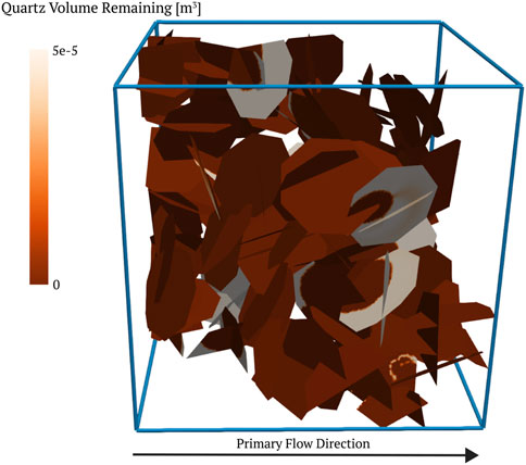
Figure 1. DFN containing 59 fractures. Fractures are colored by the remaining total quartz volume in the network at the end of the simulation.

2.2 Machine learning methods

Our goal in using ML techniques is to determine the primary factors controlling this dissolution. Regression models are valuable tools for uncovering and understanding correlations between features and observables, and in turn making accurate predictions. In this section, we present our data set, along with the derived features from the fracture network, including topological, geometric, and hydrological properties. Additionally, we provide an overview of the regression models available in Python’s scikit-learn machine learning package, and define the performance metrics used to evaluate and compare these models in the results section.

2.2.1 Flow and reactive transport data set

We used 800 generic networks for training and testing the ML regression model. Each DFN was run with four reaction rate constants, $(k)$ of 1 $\cdot 10^{-9}$ , 1 $\cdot 10^{-10}$ , 1 $\cdot 10^{-11}$ , 1 $\cdot 10^{-12}$ mol ${\text{m}}^{-2}$ ${\text{s}}^{-1}$ , equal to a total of 3256 networks. The DFNs consist of a set of fractures (on average 133 fractures per network) and each fracture is considered a sample used to train or test the random regression model. The total number of fractures in the data set is 446,129 fractures, and two-thirds (2/3) of the data were used for training the ML model (training set), while the rest of the data (1/3) were used for testing the model (testing set). The fracture-based features are divided into three categories: (i) topological, (ii) geometric, and (iii) hydrological as described below.

2.2.1.1 Topological features

To obtain and measure the topological features of the DFN, we adopt a graph-based representation as described in Hyman et al. (2018). Therein the fractures are represented as nodes in the graph, and intersections between fractures are represented as edges. If two fractures intersect in the DFN, then there is an edge in the graph between the corresponding nodes. Formally, let $\mathrm{\Omega }=\{f_i\}$ for $i=1,\dots ,N$ denote the entire network composed of $N$ fractures and let ${\ell }_{i,j}$ be the set of intersections between fractures, i.e., $f_i\cap f_j\ne \varnothing \equiv {\ell }_{i,j}$ . We define a graph $G=(V,E)$ of node set $V$ and edge set $E$ using a mapping $\varphi$ defined in the following way. For every fracture $f_i\in \{f_i\}$ , there is a node $v\in V$ ,

$\varphi :f_i\to v_i.$

Similarly, for every intersection in ${\ell }_{i,j}$ , there is an edge $e_{i,j}\in E$ that connects the corresponding nodes in $V$

$\varphi :f_i\cap f_j\ne \varnothing \to e_{i,j}=\left(v_i,v_j\right).$

We also include nodes representing the inflow and outflow boundaries $G$ to account for the direction of flow. Every fracture that intersects the inlet plane ${\mathbf{x}}_0$ is connected to the source node $s$

$\varphi :f_i\cap {\mathbf{x}}_0\ne \varnothing \to \left(s,v_i\right).$

Likewise, every fracture that intersects the outlet plane ${\mathbf{x}}_L$ is connected to the target node $t$

$\varphi :f_i\cap {\mathbf{x}}_L\ne \varnothing \to \left(v_i,t\right).$

Similar mappings have been used in the literature Hope et al. (2015); Andresen et al. (2013); Hyman et al. (2017). Note that the mapping $\varphi$ is an isomorphic bijection, which means that every sub-graph in the graph corresponds to a unique sub-network in the DFN. The graph is handled using NetworkX Hagberg et al. (2008) and all graph-based features are computed using built-in algorithms within NetworkX.

Figure 2 shows a graph representation of one DFN from our set of simulations, other networks exhibit the same behavior. We represent each DFN using a graph to characterize topological structure influences for the distribution of reactive transport within the network. In Figure 2A fractures are colored by their remaining quartz volume at the end of the simulation. There is almost no quartz remaining in fractures that are well connected between the inflow and outflow nodes. However, there remains a substantial amount of quartz in the fractures in that set’s compliment. Flow channelization, isolated regions of higher volumetric flow rates, is a commonly observed phenomenon in field and laboratory experiments as well as numerical simulations in fractured media Abelin et al. (1991); Abelin et al. (1985); de Dreuzy et al. (2012); Frampton and Cvetkovic (2011); Hyman (2020); Rasmuson and Neretnieks (1986). These flow channels indicate the existence of primary sub-networks, also referred to as backbones, within the fracture network. To this end, we partition the network into disjoint primary and secondary sub-networks. Formally, let $\mathrm{\Omega }=\{f_i\}$ for $i=1,\dots ,N$ denote the entire network composed of $N$ fractures, then

$\mathrm{\Omega }={\mathrm{\Omega }}^{\prime }\cup {\mathrm{\Omega }}^{*}\text{\hspace{0.17em}and\hspace{0.17em}}{\mathrm{\Omega }}^{\prime }\cap {\mathrm{\Omega }}^{*}=\varnothing ,$

where ${\mathrm{\Omega }}^{\prime }$ and ${\mathrm{\Omega }}^{*}$ are the primary and secondary sub-networks. We define the secondary network to be comprised of all dead-end structures, i.e., dead-end fractures and cycles, and the primary sub-network is its complement, similar to the methods proposed in Doolaeghe et al. (2020) and Yoon et al. (2023). Our partitioning definition is based solely on the network structure, specifically the topology/connectivity, and does not utilize any hydraulic, geometric, or flow information. To do so, we compute the current-flow through the network using Kirchhoff’s laws with one unit of current is injected into the graph at the source node and one unit is extracted at the target, and every edge has unit resistance. Kirchhoff’s law expresses that the sum of incoming currents at a node must be equal to the sum of outgoing currents. Defining the sign of incoming currents as positive and the sign of outgoing current as negative, the law can be represented as the sum of the currents at each node being zero,

${\displaystyle \sum _j^n}{I}_{i,j}=0\forall v_i\in V.$

Once the current is determined on every edge, all edges with current less than machine precision $(ϵ=10^{-16})$ are removed

$E^{\prime }=\left\{e_{i,j}\right\}\text{\hspace{0.17em}if\hspace{0.17em}}{I}_{i,j}>ϵ.$

Then any nodes that are no longer connected to the sub-network containing the source are removed

$V^{\prime }=\left\{v_i\right\}\text{\hspace{0.17em}if\hspace{0.17em}}|e_{i,\cdot }|>0,$

where $|e_{i,\cdot }|$ is the number of edges with an endpoint on the node $v_i$ . Then our primary sub-graph is defined as

$G^{\prime }=\left(V^{\prime },E^{\prime }\right),$

and the secondary is its complement

$G^{*}=G\backslash G^{\prime }.$

Recalling that the mapping $\varphi$ is a bijective isomorphism allows us to extract the primary and secondary sub-networks of the DFN

${\varphi }^{-1}:G^{\prime }\to {\mathrm{\Omega }}^{\prime }\text{and}{\varphi }^{-1}:G^{*}\to {\mathrm{\Omega }}^{*}.$

Figure 2B shows the same graph as in (a) but nodes are colored by their distance to the backbone. There is a correlation between the volume of quartz remaining and the distance to the backbone, indicating the latter’s impact on dissolution.

Figure 2

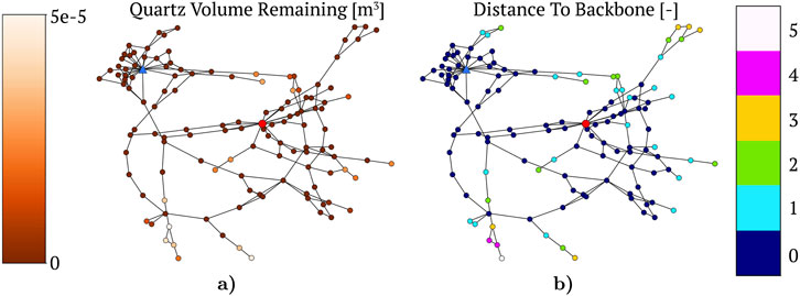
Figure 2. Graph representations based on the DFN shown above. Nodes/fractures are colored by (A) quartz volume remaining (B) topological distance to the backbone. Distance to the backbone equal to 0 refers to a fracture on the backbone (primary sub-network membership).

Based on the network connectivity, we obtain the following topological features:

1. Node degree: The degree of a node $v_i$ is the number of edges with one endpoint on the node $v_i$ . It describes the number of intersections on the corresponding fracture. Formally,

$\text{Degree}\left(v_i\right)={\displaystyle \sum _{j=1}^n}{A}_{ij},$

where $A_{i,j}$ is the adjacency matrix of the graph $G$ in which the entry $a_{i,j}$ is the number of edges in $G$ with end points $e_{i,j}=(v_i,v_j)$ . Nodes with a larger degree are well connected and ought to be a location of substantial transport and reactions.

2. Degree centrality: Degree centrality is a normalized measure of the node degree defined above. For vertex $i$ ,

$\text{Degree\hspace{0.17em}centrality}\left(v_i\right)=\frac{1}{n-1}{\displaystyle \sum _{j=1}^n}{A}_{ij}.$

High degree centrality indicates that a node is well connected and such nodes tend to be concentrated in the core of the network. Nodes with low degree centrality are often in the periphery or on branches that cannot conduct significant flow and transport. Physically, it describes the number of other fractures that intersect with a given fracture.

3. Distance to backbone: If a fracture is on the backbone, then the distance to the backbone is 0. If the fracture is in the secondary sub-network, then the value is the shortest topological path from that fracture to one on the backbone. Formally,

$\text{Distance\hspace{0.17em}to\hspace{0.17em}backbone}\left(v_i\right)=\left\{\begin{array}{cc}0,\hfill & \text{if\hspace{0.17em}}{f}_i={\mathrm{\Omega }}^{\prime }\hfill \\ \min d\left(f_i,f_j\right)\forall f_j\in {\mathrm{\Omega }}^{\prime },\hfill & \text{if\hspace{0.17em}}{f}_i\ne {\mathrm{\Omega }}^{*}\hfill \end{array}\right.$

where the topological distance metric $d(u_i,u_j)$ counts the number of edges between the nodes $u_i$ , $u_j$ . In practice, we use an unweighted Dijkstra’s method implemented in NetworkX for the search. Primary/secondary membership is a good indicator of the final quartz volume in each fracture–compare Figures 2A, B. Almost all of the quartz has been dissolved out of the primary sub-network and there is a significant volume remaining in the secondary sub-network fractures. Beyond a Boolean of backbone membership, the distance to the backbone includes more information about the proximity of a fracture in the secondary sub-network to the backbone. Reactions in fractures that are farther away from the backbone tend to be transport-limited and therein remains more quartz.

4. Betweenness centrality: The betweenness centrality Anthonisse (1971); Freeman (1977) of a node describes the extent to which a node can control communication on a network. Consider a path with the fewest possible edges (geodesic path), that connects a node $u$ and a node $v$ on a graph. In general, there may be more than one such paths, and with ${\sigma }_{uv}$ , we denote the number of such geodesic paths. Furthermore, let ${\sigma }_{uv}(i)$ denote the number of such paths that pass through node $i$ . We then define for node $i$ ,

$\text{Betweenness\hspace{0.17em}centrality}=\frac{1}{\left(n-1\right)\left(n-2\right)}{\displaystyle \sum _{\begin{array}{c}u,v=1\\ u\ne i\ne v\end{array}}^n}\frac{{\sigma }_{uv}\left(i\right)}{{\sigma }_{uv}},$

where the leading factor normalizes the quantity so that it can be compared across graphs of different sizes $n$ . Many backbone nodes have high betweenness values; however, other paths through the network can show high values, since this feature considers all paths in the graphs, and not only those from source to target.

5. Source-to-target current flow: This is a type of centrality measure adopted from an electrical current model Brandes and Fleischer (2005). The current flow assumes a given source and target. Imagine that one unit of current is injected into the network at the source, one unit is extracted at the target, and every edge has one unit of resistance. Then, the current flow centrality is given by the current passing through a given node. This can be described by Kirchhoff’s laws, or in terms of the graph Laplacian matrix $\mathbf{L}=\mathbf{D}-\mathbf{A}$ , where $\mathbf{A}$ is the adjacency matrix for the graph and $\mathbf{D}$ is a diagonal matrix specifying node degree: $D_{ii}={\sum }_j{A}_{ij}$ . We can define the current flow for node $i$ as

$\text{Current\hspace{0.17em}flow\hspace{0.17em}}\left(v_i\right)={\displaystyle \sum _{j=1}^n}{A}_{ij}\left|\left(L_{is}^{+}-L_{js}^{+}\right)-\left(L_{it}^{+}-L_{jt}^{+}\right)\right|,$

where ${\mathbf{L}}^{+}$ is the Moore-Penrose pseudoinverse of $\mathbf{L}$ , $s$ is the source node, and $t$ is the target node.

The current flow centrality is often referred to as random-walk centrality Newman (2005), measuring how often a random walk from the source $(s)$ to the target $(t)$ passes through a node $i$ . Unlike betweenness centrality, the current flow centrality considers only the paths from source to target, its values are zero on any branch of the graph outside of the central core. Thus, we expect a correlation between high current flow values and nodes that have a large influence on the transport from source to target.

2.2.1.2 Geometric features

The following features are based on the fracture geometry. Recall that fractures are planar discs with the same initial aperture and radius. Thus, initially, they all have the same surface area and volume. However, if a fracture intersects with the domain boundary, its shape is modified to conform to the boundary. Therefore, there is variation in the following attributes.

1. Surface area: The surface area of the polygon represents the fracture plane. For a non-truncated fracture, the value is equal to $\pi r^2$ .

2. Total fracture volume: The total volume of the fracture is the surface area, which varies between fractures, and the aperture, which is initially constant,

$\text{Total\hspace{0.17em}fracture\hspace{0.17em}volume\hspace{0.17em}}{n}_i=V_i.$

The total fracture volume determines the initial amount of quartz in each fracture, being the total volume multiplied by the initial volume fraction (80%). Because the total quartz volume is a constant scaled quantity of the total fracture volume, we only include the total fracture volume as a feature.

3. Projected volume: The projected volume of the fracture is the component of a fracture’s volume-oriented parallel to the main flow direction (inlet to outlet plane). Assuming the flow is oriented along the $x$ -axis, the projected volume is expressed as

$\text{Projected\hspace{0.17em}volume}=V_i\sqrt{{\left({\mathbf{O}}_i\right)}_y^2+{\left({\mathbf{O}}_i\right)}_z^2},$

where $V_i$ is the volume of fracture $i$ and ${\mathbf{O}}_i$ is the unit vector normal to the fracture plane, called the orientation vector. Since the flow is oriented along the $x$ -axis, the projected volume is expressed by the projection of ${\mathbf{O}}_i$ onto the $yz$ -plane. Fractures that are oriented along the main flow direction are more likely to carry a significant part of the flow, compared to the fractures oriented perpendicular to the normal flow direction.

4. Intersection area: The intersection area is the total length of intersections on a fracture multiplied by the initial aperture.

2.2.1.3 Hydrological features

The following are a set of hydrological features that are computed on a pipe-network representation of the DFN, cf. Karra et al. (2018) for details on how the pipe/graph-network is obtained and how the numerical simulations are performed. Steady pressure-driven flow is computed to obtain pressure and volumetric flow rates throughout the DFN. Obtaining these values is computationally inexpensive especially when compared to the high-fidelity reactive transport simulations.

1. Volumetric flow rate: We compute the volumetric flow rate of fluid passing through each fracture. Given the flow rates into and out of the fracture, we take a single value that is one-half the absolute value of total flow exchanged by a fracture with its neighbors,

$Q\left(f_i\right)=\frac{1}{2}{\displaystyle \sum _j^n}|Q_{i,j}|.$

The absolute value is necessary because of the sign dependence of flow into (positive) and outgoing (negative), and the 1/2 is to account for double counting.

2. Péclet number: We compute the Péclet number of each fracture using the volumetric flow rate $Q_i$ , fracture radius $r_i$ , surface area $S_i$ and the diffusion coefficient $D=10^{-12}{\mathrm{m}}^2/\text{s}$

$Pe\left(f_i\right)=\frac{Q_i{r}_i}{S_{i}D}.$

Regions with a high Péclet tend to occur within the primary sub-network and reactions therein are kinetically-limited, i.e., there is sufficient volumetric flow to flush away the aqueous silica, and once the quartz is fully dissolved in the primary sub-network, than a quasi-steady state is reached, and the overall apparent dissolution rate slows.

3. Advective Damköhler number: The advective Damköhler number compares the reaction timescale to the convection. We compute it on a fracture basis, similar to the Péclet number. First, we convert the rate constant $k$ [mol ${\text{m}}^2$ /s] used in simulations to a rate $k^{\prime }$ [m/s] using the quartz molar volume (V $\text{m}$ = 22.6880 $10^{-6}$ ${\text{m}}^3$ /mol, $k^{\prime }=kV\text{m}$ ). Then our advective Damköhler number is defined as

$D{a}_I\left(f_i\right)=\frac{k^{\prime }{S}_i}{Q_i}.$

4. Diffusive Damköhler number: Likewise, we compute the diffusive Damköhler which compares the reaction timescale to diffusion and is given as

$D{a}_{II}\left(f_i\right)=\frac{k^{\prime }{r}_i}{D}.$

This concludes the definition of the input features used to train the ML regression models as described in the following sections.

2.2.2 Regression models

Regression models are powerful tools enabling prediction, analysis, and optimization of various phenomena. They are often used to understand the relationship between a target variable and the features of the data set. The main goal of the regression models is to predict the target value based on the input features. Types of regression models include linear regression, ridge and lasso (least absolute shrinkage and selection operator) regression, polynomial regression, support vector regression, decision tree regression, random forest regression, gradient boosting regression, and HistGradientBoostingRegressor James et al. (2013). Based on the complexity of our data set and the large number of input features, we focus on support vector regression, decision tree regression, random forest regression and gradient boosting regression, since these models are capable of handling more complex non-linear relationships. Table 1 includes a summary of the regression models considered in this study.

Table 1

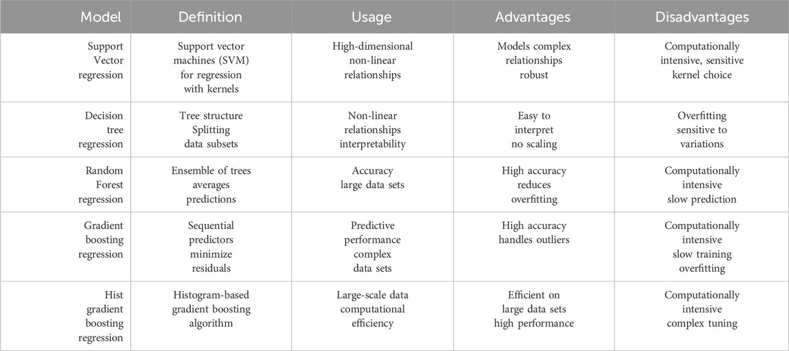
Table 1. Summary of regression models used in this study.

All these regression models also provide an importance estimate of the individual features, also called permutation importance. To measure the feature’s importance the values of each feature are randomly permuted; a decrease in performance compared to the baseline indicates the importance of the permuted features. The importance score is calculated by averaging the difference between the error before and after the feature permutation. If a feature is important for the regression model, the permutations will produce many errors, while if a feature is not important, the permutations will not have a large effect on the performance of the regression method. We show the results of the importance analysis in Section 3.3.

To assess the performance of the regression models, we use the R-squared score (R2), also called coefficient of determination. In regression models, the R2 coefficient measures how well the regression predictions estimate the real data points. An R2 coefficient of determination equal to 1.0 signals that the predictions of the regression model perfectly fit the data.

In Section 3, we compare the different regression models and their performance taking into account the before mentioned performance measures. We discuss the correlations between features, as well as the accuracy of the trained ML models. For all our ML studies we use the scikit-learn machine learning package developed in Python Pedregosa et al. (2011).

3 Results

We use the flow and reactive transport data set described in Section 2.2.1 to train multiple regression models in order to predict the quartz volume that remains in a given fracture depending on three different attribute sets–topological, geometric, and hydrological features as described above. In our ML models, we also include the reaction rate constant, which we consider a primary control feature. The results show that having access to flow features enhances the accuracy of the quartz volume prediction, however, it is not significant.

In the next subsection, we perform a comparison between different regression models. Once we identify the most suitable regression model (random forest regression model) for our data set, we perform an extensive grid search to obtain an optimized version of the model. In Section 3.3, we discuss the feature importance analysis, giving us insights into the significance of each feature in predicting the remaining quartz volume per fracture. This analysis shows an interplay between the feature categories and their correlations. Later, we show details on the performance of the following two types of random forest regression models: (1) including all rate constants and gradually adding more complexity regarding the feature categories. For this type, we generated the following three regression models: RF-1 model using only topological features; RF-2 model using topological and geometric features; RF-3 model using topological, geometric, and hydrological features; (2) including one rate constant at a time while using all features, resulting in four regression models for each of the rate constants.

3.1 Regression models comparison

As mentioned in Section 2.2.2, we trained the following regression models: support vector regression, decision tree regression, random forest regression and two versions of the gradient boosting regression. For the training, we included all the features, and we used the default parameters for each of the regression models as specified in the scikit-learn online documentation. Table 2 shows the R2 values for the training and testing.

Table 2

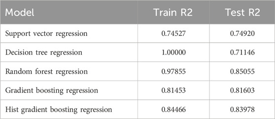
Table 2. Comparison of the regression models’ performance.

The random forest method outperforms the other regression models, when considering the R2 test results. The random forest method uses an ensemble of recursively defined decision trees at training time. Each tree considers a random portion of the original data as training and the output of the method is the mean prediction of the individual trees Watt et al. (2020). Combining forests of trees can produce a single high-performing model and is suitable for large data sets Ho (1995).

In the rest of the paper, we focus on training random forest regression models using different combinations of features.

3.2 Grid search

The random forest regression model can be further optimized to obtain even better R2 scores by tuning the hyperparameters of the model. We performed an exhaustive cross-validated grid search over a number of parameter values using the GridSearchCV function. The optimized model was obtained after a grid search through the following hyperparameters: n_estimators, max_depth, max_features, min_samples_leaf, and min_samples_split. The ranges for each of these hyperparameters are given in Table 3. The input parameters used for the grid search study include all features: topological, geometric, hydrological, and the reaction rate constant (RF-3).

Table 3

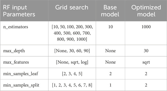
Table 3. Hyperparameter ranges for the cross-validate grid search and results. We show the default parameters used for the base model, as well as the optimized hyperparameters, resulting from the grid search. To obtain these results, we use the RF-3 model, which contains all input features (topological, geometric, hydrological, and the reaction rate constant). Additionally, we set the following parameters for all regression models: bootstrap=True, and oob_score=True.

The cross-validated grid search took approximately 20 h to complete on a CPU machine. Training the R3 base model took about 20 s, whereas the optimized model required around 7.5 min on the same machine. This increase in time is primarily due to the higher number of estimators used in the optimized model. Although the optimized model is nearly 22 times slower, it is significantly more robust and less prone to overfitting.

Table 4 shows a performance comparison between the base model (using the default parameters for the RandomForestRegressor function) and the optimized model considering the R2 value obtained during training and testing, and the out-of-bag score, which is an unbiased estimate of the model’s performance during training. The out-of-bag score is calculated by averaging only the trees for which a given data point prediction was not in the training data. This score is only available when bootstrap=True, which means that bootstrap samples are used when building the trees instead of using the whole data set for each tree. We enabled the out-of-bag score using the following command oob_score=True.

Table 4

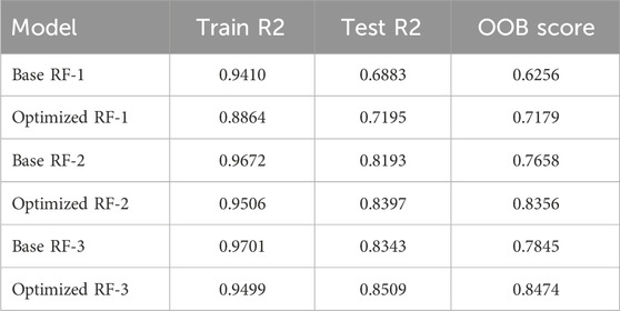
Table 4. Performance measures of the random forest regression models. Comparison between the base regression model, using the default parameter values, and the optimized model, obtained from an exhaustive cross-validated grid search. These random forest models use all rate constants, while the number of input features is increased gradually with each model. The optimized model performs better than the base model. The improved out-of-bag (OOB) score, which measures model performance using data not included in the training subset, confirms the optimized model’s superiority.

The performance measured in Table 4 shows that the remaining quartz volume is hard to predict. When using only the topological features (RF-1 model), the random forest regression models (base and optimized) perform poorly, indicating that the topological features do not carry enough information to train the model. Adding geometric features enhances significantly the performance of the base and the optimized model. The R2 train values of the optimized model actually decrease in comparison to the base model; however, this is because the base model is overfitting. Including hydrological features (RF-3 model) only slightly increases the accuracy of the models, pointing to the complexity of the DFN system exhibiting dissolution.

The overall accuracy of the training for the base and the optimized model is good, however, during testing the coefficient of determination (R2 value) drops significantly. This is very clear for the RF-1 base model, where only topological input features are used. The train R2 score for RF-1 is 0.9410, while during testing the model’s test R2 score is only 0.6883, which implies that the random forest regression models overfit during training and show higher accuracy in training while under-performing during testing. The optimized models overfit less and perform slightly better than the base model. The small difference between the test R2 values of the base and the optimized model suggests that performing a grid search and tuning the model parameters, even though important, it might not improve the accuracy of the training significantly. This strongly depends on the data set and the problem at hand.

The out-of-bag score (OOB) measures the model performance using data not included in the training subset. The OOB score of the optimized model is eight to nine points greater than the one of the base model, which confirms that the optimized model is more reliable than the base model, since higher OOB score reflects better agreement and is desirable.

3.3 Feature importance analysis

As mentioned previously the random forest regression model can be used to identify the importance of each individual feature for the performance of the trees. Figure 3 depicts the input feature importance analysis results for the three random forest regression models (RF-1, RF-2, and RF-3), with a gradually increasing number of features. Each model uses all values of the rate constant, shown in black. The topological features are displayed in orange, the geometrical features in purple, and the hydrological features in green.

Figure 3

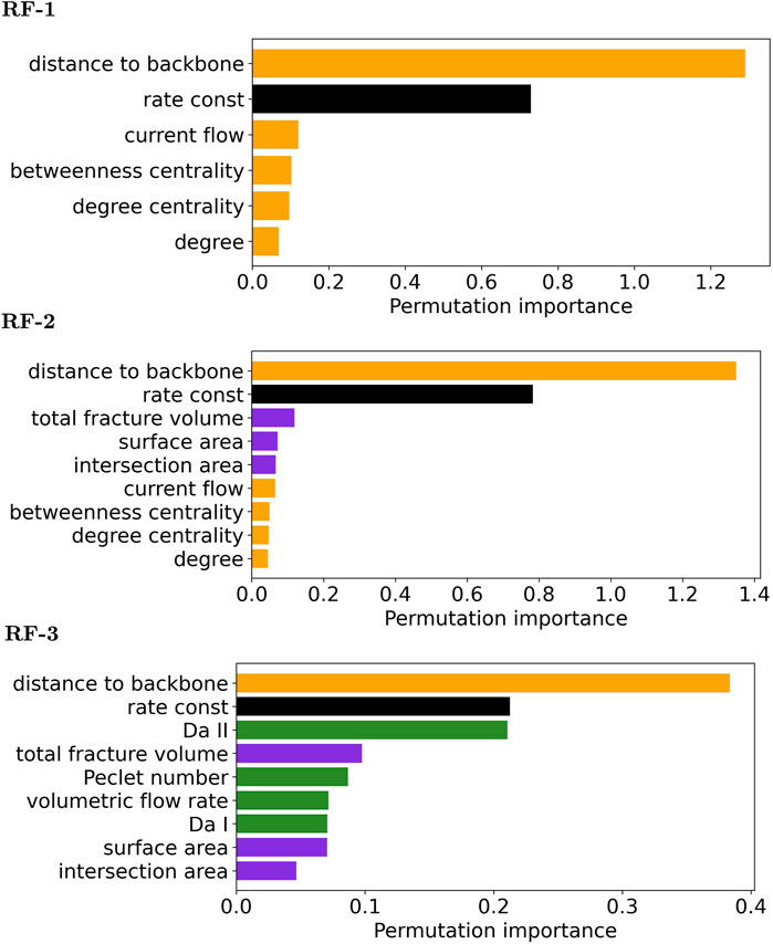
Figure 3. Feature importance analysis for three regression models: RF-1 (topological features), RF-2 (topological and geometric features), and RF-3 (hydrological, topological and geometric features). The topological features are depicted in orange, the geometric features in purple, the hydrological features in green, and the reaction rate constant in black. The importance analysis for all models show that the distance to the backbone and the rate constant are the most important features in our study.

The feature importance analysis is calculated by comparing the baseline model to the model obtained by permuting the feature column. As shown in Figure 3, the analysis confirms that the distance to the backbone and the rate constant are the two main quantities controlling the dissolution of quartz in the fractures for all regression models. This is not surprising since the distance to the backbone indicates how far a fracture is with respect to the backbone. The transport in fractures that are farther away from the backbone tend to be diffusion-dominated, thus therein remains more quartz. Likewise, when a given fracture is part or in the vicinity of the primary sub-network, the behavior in the fracture is advection-dominated, which leads to the complete depletion of quartz within the fractures. The rate constant is the second important feature for all trained regression models because it indicates the strength of dissolution in the fracture. There is a strong correlation between the distance to the backbone, reaction rate, and the quartz volume that remained in the system, since as the reaction rate increases also the dissolution penetrating deeper levels of the secondary fracture sub-network. This means that as higher the rate constant is, the more quartz will be flushed out from the secondary sub-network (taking into account that all quartz is dissolved from the primary sub-network). Conversely, when the rate constant is small, the reactive transport is reduced almost entirely to the primary sub-network.

As we increase the number of features from topological to topological and geometric, we can see that the total fracture volume, surface area and intersection area line up right after the first two topological features. When we add hydrological features, we observe that the diffusive Damköhler number ( ${\text{Da}}_{II}$ ) becomes almost as important as the rate constant, followed by the total fracture volume and other hydrological features. From the training results shown in Table 4, we know that the model accuracy does not improve drastically, when more features are included in the training; however, from the features importance analysis, we can confirm that they carry significant information for the flow and reactive transport of a fracture. Reactions during early simulation times are kinetically-limited occurring mostly in the primary network. However, once all of the quartz in the primary network is dissolved, the secondary network becomes the location where all reactions are occurring. Flow in the secondary network is slow compared to the primary network (Péclet number $<1$ ) and reactions therein are transport-limited rather than kinetically. Thus, reactions in the secondary network are a balance between diffusion and the reaction rate, which is diffusive Damköhler number measures. In other words, ${\text{Da}}_{II}$ captures the integrated effects of the distance to the backbone, rate constant, and Péclet number into a single variable which is then linked with late time dissolution effects and prediction of the remaining quartz in the system.

Figure 4 shows the correlations between input features (correlation matrix) in our regression model as a heat map. We omitted the correlation matrix for the RF-1 model since the topological features are depicted in RF-2 and RF-3. We reduced the number of features for each heat map to ten to improve readability.

Figure 4

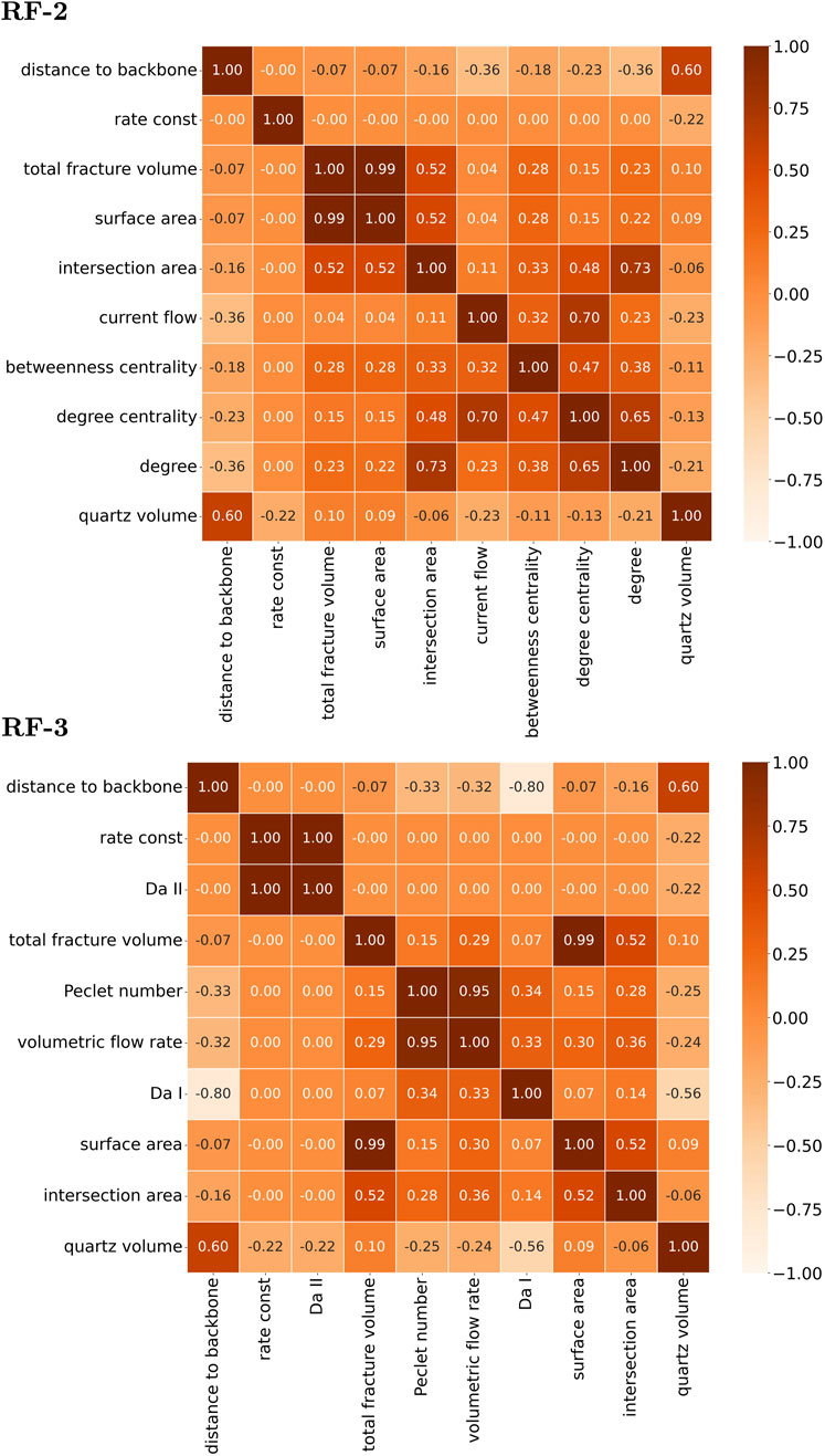
Figure 4. Correlation matrix of the model features displayed as a heat map for the remaining quartz and the first nine features used for the random forest regression training. The RF-2 results show strong correlations between the following features: distance to the backbone and the quartz volume, total fracture volume and surface area, intersection area and degree, current flow, and degree centrality. The RF-3 model shows a strong correlation between the aforementioned features and the following hydrological features: ${\text{Da}}_{II}$ and rate constant, volumetric flow rate and Péclet number. We observe a strong inverse correlation between ${\text{Da}}_I$ and the distance to the backbone, and ${\text{Da}}_I$ and quartz volume. The RF-1 model is omitted for clarity.

The results for RF-2 show strong correlations between the following features: total fracture volume and surface area (0.99), intersection area and degree (0.73), current flow and degree centrality (0.70), degree centrality and degree (0.65), and distance to the backbone and the quartz volume (0.60). When we add the hydrological features, some of the less significant topological features are not displayed. The RF-3 model show strong correlation between the aforementioned features and the following hydrological features: diffusive Damköhler number ( ${\text{Da}}_{II}$ ) and rate constant (1.0), volumetric flow rate and Péclet number (0.95). We observe a strong inverse correlation between the advective Damköhler number ( ${\text{Da}}_I$ ) and the distance to the backbone (−0.8), and the advective Damköhler number ( ${\text{Da}}_I$ ) and the quartz volume (−0.56). This is expected since these variables are derived from one another, and it confirms that the regression models learn the correct behavior by being able to predict those strong correlations.

3.4 Regression models using all rate constants

Training regression models on all rate constants allows for comparison between different feature categories. Figure 5 shows the train and test results for the RF-1, RF-2, and RF-3 models.We see that using only the topological features is not sufficient to obtain a good regression model. The RF-1 test results are scattered and the model is not able to predict the correct target quartz values. By adding the geometric features (RF-2 model), we observe much better predictions of the remaining quartz volume. However, the random forest regression model still has difficulties predicting the quartz volume, especially when the quartz is either fully depleted or clogs the fracture (normalized quartz volume close to 0 or 1, respectively) in advection- or diffusion-dominated regions, respectively. We trained a third model (RF-3) that includes the hydrological features, which performs slightly better than the RF-2 model; however, the improvement is not significant. While hydrological features contribute to model predictions, their relatively lower importance suggests that structural and geometric features are more critical in controlling flow and reactive transport dynamics.

Figure 5

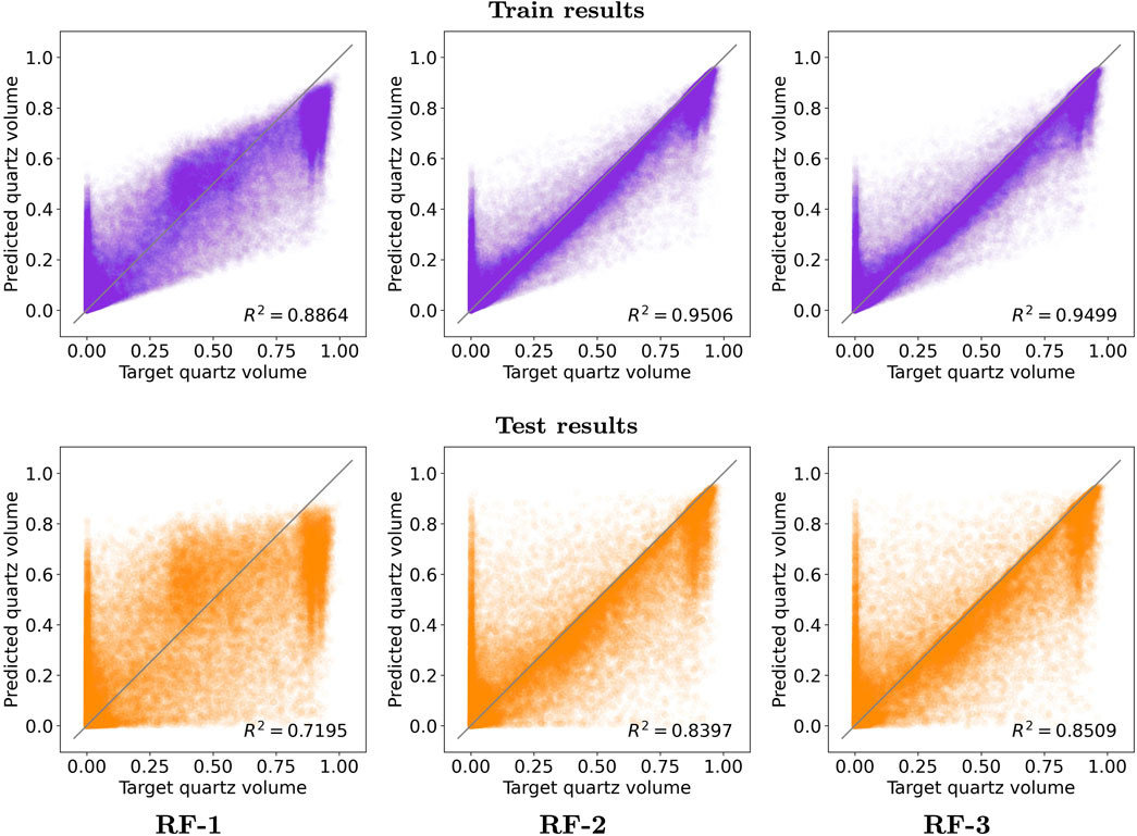
Figure 5. Random forest train (purple) and test (orange) predictions for the following models: RF-1 (topological features), RF-2 (topological and geometric features), and RF-3 (hydrological, topological, and geometric features). The RF-1 model does not include enough input parameters to predict correctly the remaining quartz volume in a given fracture. RF-2 shows tighter predictions; however, it still fails to predict the quartz volume for fractures that are either fully depleted or clogged (normalized quartz volume close to 0 or 1, respectively). RF-3 gives slightly better predictions (see the R2 score); however, the improvement is not significant.

3.5 Regression models using a single rate constant

In order to have a better grasp on why training a regression model using all rate constants does not deliver a very accurate prediction for the quartz volume remaining in each fracture, we train four more random forest regression models using all input features and one rate constant at a time. The coefficient of determination (R2 score) during training and testing is depicted in Figure 6.One can see that the random forest regression model has difficulties predicting the remaining quartz volume for large rate constants, (k) of 1 $\cdot 10^{-9}$ and 1 $\cdot 10^{-10}$ mol ${\text{m}}^{-2}$ ${\text{s}}^{-1}$ , while for small rate constants, (k) of 1 $\cdot 10^{-11}$ and 1 $\cdot 10^{-12}$ mol ${\text{m}}^{-2}$ ${\text{s}}^{-1}$ , the model performs significantly better. When the rate constant is large, we expect more rapid quartz dissolution as fresh water is introduced to the system. This results in advection-dominated flow and quartz depletion in the backbone of the DFN, leading to shorter reactive transport simulation times since the quasi-steady state is reached in less time. It might seem a bit counter-intuitive, but for large rate constants the quartz volume in the system will be either flushed out completely from the fracture (mostly in a close proximity to the backbone, advection-dominated flow), or it will be clogging the fractures to a high extend (mostly in the secondary sub-network, diffusion-dominated flow), leading to sharp interfaces between the primary and the secondary sub-networks. This effect can be seen in Figures 6A, B, where most of the samples are located either in the lower left or in the upper right corners. The figures seem to have fewer data samples, but this is not the case, the data points are simply overlapping in the aforementioned regions. This makes predicting the remaining quartz volume for a single fracture much harder for the regression model since the distance to the backbone feature will carry less significant information.

Figure 6

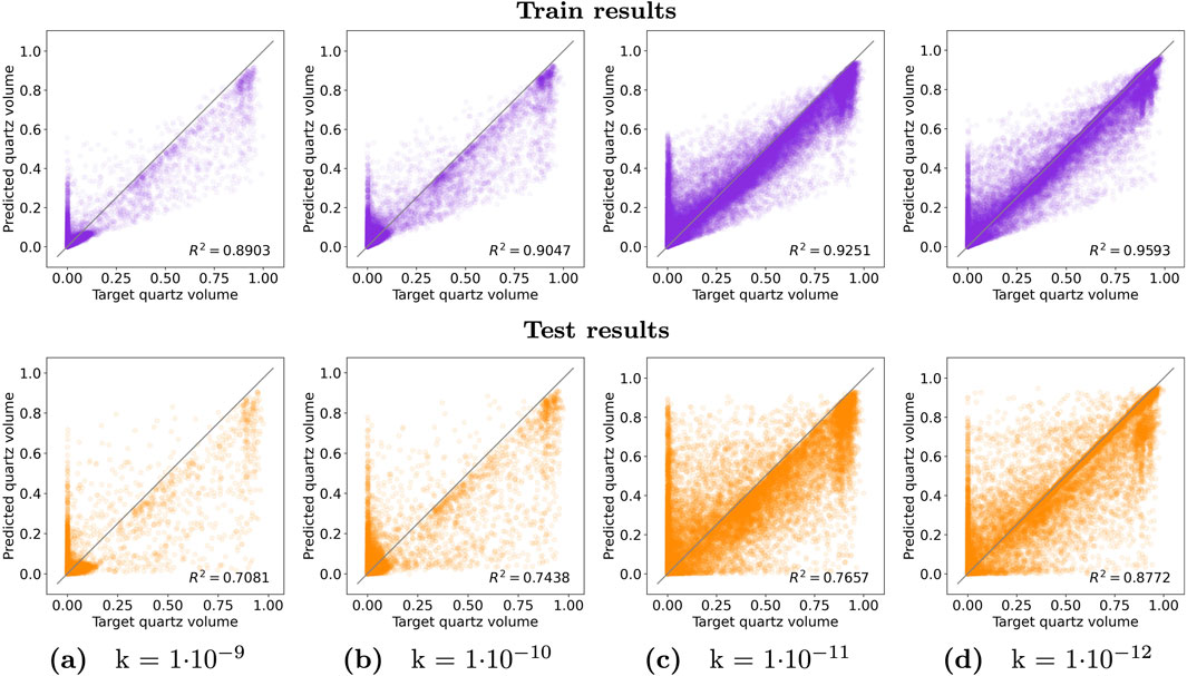
Figure 6. Random forest train and test predictions for each of the rate constants using all features (geometrical, topological, and hydrological). Each column depicts the results for a different rate constant (A–D). The regression model can predict the remaining quartz volume with higher accuracy for lower rate constants. The reaction rate constant is in ( ${\mathbf{m}\mathbf{o}\mathbf{l}\mathbf{m}}^{-\mathbf{2}}$ ${\mathbf{s}}^{-\mathbf{1}}$ ) units and each train/test model has an equal number of data samples.

Reaching a quasi-steady state for simulations with lower reaction rates, (k) of 1 $\cdot 10^{-11}$ and 1 $\cdot 10^{-12}$ mol ${\text{m}}^{-2}$ ${\text{s}}^{-1}$ , takes longer times since the reactions within fractures are slower. For those systems, we observe much smoother interfaces between the quartz-filled and quartz-depleted regions. This allows a smoother transition between these regions and more variability in the distance to the backbone feature, making the prediction of the remaining quartz volume an easier task. This is displayed in Figures 6C, D, where the data samples are almost equally distributed in the range of quartz volume. In this case, the regression model predicts the remaining quartz volume with higher accuracy.

4 Discussion

This study provides valuable insights into the factors controlling mineral dissolution in fractured media, with implications for geologic carbon sequestration. By leveraging machine learning techniques and high-fidelity simulations of reactive transport, we identified the dominant features influencing quartz dissolution and developed predictive models with promising accuracy. Below we discuss (1) the advantages and limitations of the methodology; (2) insights on controlling factors in mineral dissolution; and (3) the implications for geologic sequestration.

4.1 Advantages and limitations of the methodology

The random forest regression model outperformed the other regression models that we tested (support vector regression, decision tree regression, random forest regression and two types of gradient boosting regression). An key advantage of using the random forest regression model is that it provides importance rankings, which lead to insights into the system behavior. A similar approach was taken by Valera et al. (2018a) when considering the prediction of backbone membership in a DFN, and extends their applicability by focusing on predictive modeling.

However, several limitations must be acknowledged. First, while the optimized random forest model provides more robust predictions, it is computationally intensive, running approximately 22 times slower than the base model. Second, our models are trained on limited datasets focused on dissolution and constrained to a relatively small fracture network property range, limiting their generalizability to other geochemical contexts.

4.2 Insights on controlling factors in mineral dissolution

We observe that the reaction rate constant and the distance to the backbone are the two most important features for predicting the remaining quartz volume in a single fracture. This is in agreement with the work of Andrews et al. (2023) who found that the topological structure and reaction rates were the primary factors controlling quartz dissolution in the fracture networks they considered.

The model has a hard time predicting the quartz volume remaining in a fracture using only topological features. However, adding geometric features improves the predictions significantly. Interestingly, including the hydrological features only slightly improves the regression model predictions, which suggests that structural and geometric features are more critical in controlling flow and reactive transport dynamics. In all models the distance to the backbone (a topological feature) was the most useful for prediction. This feature thereby provides a foundation for the other properties to refine upon. This identified hierarchy of lengths scales within the fracture network is agreement with other approaches characterizing non-reactive transport modeling in fractured media, which identified that the topology is the primary control, then geometry, and finally hydrological properties Maillot et al. (2016); de Dreuzy et al. (2012); Hyman and Jiménez-Martínez (2018).

High reaction rates, $(k)$ of 1 $\cdot 10^{-9}$ and 1 $\cdot 10^{-10}$ mol ${\text{m}}^{-2}$ ${\text{s}}^{-1}$ , result in sharper interfaces between the quartz-filled and quartz-depleted fractures within a DFN while lower reaction rates, $k=$ 1 $\cdot 10^{-11}$ and 1 $\cdot 10^{-12}$ mol ${\text{m}}^{-2}$ ${\text{s}}^{-1}$ , lead to smoother interfaces of quartz volume between the quartz-filled and quartz-depleted fractures within a DFN. In the former the backbone is completely depleted, while the fractures in the secondary sub-network are still filled with quartz. These reactive transport simulations take a shorter time to reach a quasi-steady state. The distance to the backbone, which we observe to be one of the most important features predicting the remaining quartz volume, becomes less significant as the quartz volume associated with it is either 0 or close to 1, as there is almost no variability in the overall network. In the case of the lower reaction rates, the simulation takes longer times to reach a quasi-steady state and the fresh water can penetrate deeper into the secondary network and dissolve larger amounts of the quartz in these fractures. These links between network structure and where reactions occur has identified through direct observation by Andrews and Navarre-Sitchler (2021); Hyman et al. (2024b); Hyman et al. (2022a); Pandey and Rajaram (2016). But this work is the first to identify such links using a data-driven approach. In these cases, the distance to the backbone and the quartz volume associated with a specific fracture carries more variability and as such serves as a stronger predictor of the quartz volume compared to the same feature when high reaction rates are used. The occurrence of sharp interfaces could become more important if precipitation is considered as the could lead to system clogging.

5 Conclusion

We conducted numerical simulations combined with regression modeling to investigate the interplay between network geostructure and geochemical reactions in fractured media. Using generic three-dimensional fracture networks, we simulated flow and reactive transport at multiple reaction rates to identify key factors controlling quartz dissolution. Combining DFN graph representation with machine learning, we identified the random forest regression model as the best performer, optimized its hyperparameters, and analyzed feature importance. We found a strong correlation between the distance to the backbone, reaction rate, and quartz volume. Finally, we built two model types: one using all rate constants with varied feature categories and another trained on individual rate constants.

Our key findings are summarized as follows:

$•$ The random forest regression model demonstrated superior performance compared to the other regression models we tested, including support vector regression, decision tree regression, and two types of gradient boosting regression.

$•$ The first type of ML models assessed the importance of each input feature category (topological, geometric, and hydrological). The results showed that building a regression model to predict the remaining quartz volume for all reaction rate constants is a difficult endeavor.

$•$ We observed that including topological and geometric features are instrumental in building a useful regression model predicting the remaining quartz volume in a quasi-steady state. Including the hydrological features are the least important ones, since they only slightly improve the accuracy of the regression models.

$•$ The most important features controlling the quartz dissolution are the rate constant and the distance to the backbone (primary sub-network), which can be easily explained, since they control the flow channelization and the strength of the chemical reaction, respectively.

$•$ The second type of ML models gave us insights on how the rate constant controls the dissolution in the DFN. The random forest regression model was able to predict the remaining quartz volume much better for low reaction rates in comparison to high reaction rates. This is due to smoother interfaces between the quartz-filled and quartz-depleted regions in the simulations using low rate constants, allowing for more variability in the quartz volume with respect to the distance to the backbone, which helps to build a more accurate model.

$•$ In all models, the distance to the backbone (a topological feature) emerged as the most significant predictor. This feature serves as a foundational element upon which other properties can build and refine their contributions.

As is slowly becoming better understood, our results reiterate that network connectivity is at the top of the hierarchy in determining flow and transport properties in fractured media. A primary contribution of this work is characterizing how that hierarchy influences reactions in fractured media as well. To this end, we observe the dynamic reactions in the system exhibit a strong interplay with the topology, geometry, and hydrology of the network. In summation, the complex structure of the fracture network determines the flow field which is then dynamically modified by the reactions. However, it is currently unknown how the inclusion of precipitation which could lead to blocking would influence these results. It is feasible that the feedback loop of precipitation leading to lowering permeability could alter the importance of our determined features. Thus, the next step in this line of research is twofold.

$•$ We need to characterize how changing fracture network properties influences our predictive capabilities as well as feature importance. To do so, one would need to build an extensive training set for different geological scenarios, rock types and family configurations.

$•$ A gradual increase in chemical complexity is required to take these insights into the field. For example, it is now possible to consider coupled mineral precipitation and dissolution in three-dimensional fracture networks Neil et al. (2024); Nisbet et al. (2024); Hyman et al. (2024a). In turn, could design similar machine learning workflows as those presented here to characterize various factors in those more complex geochemical scenarios.

Both of these avenues warrant further exploration and detailed research. Future work could also explore incorporating ensemble learning or physics-informed neural networks to capture additional dynamics in quartz dissolution and improve prediction accuracy. Additionally, increasing the size of the dataset by simulating more diverse fracture networks and reaction conditions could enhance the model’s ability to generalize across different scenarios.

Data availability statement

The raw data supporting the conclusions of this article will be made available by the authors, without undue reservation.

Author contributions

AP: Conceptualization, Data curation, Formal Analysis, Funding acquisition, Investigation, Methodology, Resources, Software, Validation, Visualization, Writing–original draft, Writing–review and editing. JH: Formal Analysis, Software, Supervision, Writing–original draft, Writing–review and editing. DO: Supervision, Writing–review and editing. GS: Funding acquisition, Supervision, Writing–review and editing. HV: Funding acquisition, Supervision, Writing–review and editing.

Funding

The author(s) declare that financial support was received for the research, authorship, and/or publication of this article. JDH, GS and HV thank the Department of Energy (DOE) Basic Energy Sciences program (LANLE3W1) for support. AAP, JDH, and HV also gratefully acknowledge support from the LANL LDRD program office Grant Number #20220019DR. AAP, DO, JDH, and HSV also gratefully acknowledge support from the LANL LDRD program office Grant Number #20250637DI. DO thanks the Department of Energy (DOE) Basic Energy Sciences program (LANLECA1) for support. AAP acknowledges the Center for Non-Linear Studies at Los Alamos National Laboratory. Research was supported as part of the Center on Geo-process in Mineral Carbon Storage, an Energy Frontier Research Center funded by the U.S. Department of Energy (DOE), Office of Science, Basic Energy Sciences (BES), under Award #DE-SC0023429. Los Alamos National Laboratory is operated by Triad National Security, LLC, for the National Nuclear Security Administration of U.S. Department of Energy (Contract No. 89233218CNA000001). Assigned LA-UR-23-33803.

Conflict of interest

The authors declare that the research was conducted in the absence of any commercial or financial relationships that could be construed as a potential conflict of interest.

Publisher’s note

All claims expressed in this article are solely those of the authors and do not necessarily represent those of their affiliated organizations, or those of the publisher, the editors and the reviewers. Any product that may be evaluated in this article, or claim that may be made by its manufacturer, is not guaranteed or endorsed by the publisher.

References

Abbasi, J., Moseley, B., Kurotori, T., Jagtab, A. D., Kovscek, A. R., Hiorth, A., et al. (2024). History-matching of imbibition flow in multiscale fractured porous media using physics-informed neural networks (pinns). arXiv Prepr. arXiv:2410.20801. doi:10.48550/arXiv.2410.20801

CrossRef Full Text | Google Scholar

Abelin, H., Birgersson, L., Moreno, L., Widén, H., Ågren, T., and Neretnieks, I. (1991). A large-scale flow and tracer experiment in granite: 2. results and interpretation. Water Resour. Res. 27, 3119–3135. doi:10.1029/91wr01404

CrossRef Full Text | Google Scholar

Abelin, H., Neretnieks, I., Tunbrant, S., and Moreno, L. (1985). Final report of the migration in a single fracture: experimental results and evaluation. Nat. Genoss. Fd. Lager. Radioakt. Abfälle.

Google Scholar

Ahmmed, B., Mudunuru, M. K., Karra, S., James, S. C., and Vesselinov, V. V. (2021). A comparative study of machine learning models for predicting the state of reactive mixing. J. Comput. Phys. 432, 110147. doi:10.1016/j.jcp.2021.110147

CrossRef Full Text | Google Scholar

Andresen, C. A., Hansen, A., Le Goc, R., Davy, P., and Hope, S. M. (2013). Topology of fracture networks. Front. Phys. 1 (Art–7). doi:10.3389/fphy.2013.00007

CrossRef Full Text | Google Scholar

Andrews, E., Hyman, J., Sweeney, M., Karra, S., Moulton, J., and Navarre-Sitchler, A. (2023). Fracture intensity impacts on reaction front propagation and mineral weathering in three-dimensional fractured media. Water Resour. Res. 59, e2022WR032121. doi:10.1029/2022wr032121

CrossRef Full Text | Google Scholar

Andrews, E., and Navarre-Sitchler, A. (2021). Temporal and spatial heterogeneity of mineral dissolution rates in fractured media. Geochimica Cosmochimica Acta 312, 124–138. doi:10.1016/j.gca.2021.08.008

CrossRef Full Text | Google Scholar

Anthonisse, J. M. (1971). “The rush in a directed graph,” in Stichting mathematisch centrum. Amsterdam, Netherlands: Mathematische Besliskunde.

Google Scholar

Atchley, A. L., Maxwell, R. M., and Navarre-Sitchler, A. K. (2013). Using streamlines to simulate stochastic reactive transport in heterogeneous aquifers: kinetic metal release and transport in CO2 impacted drinking water aquifers. Adv. Water Resour. 52, 93–106. doi:10.1016/j.advwatres.2012.09.005

CrossRef Full Text | Google Scholar

Becker, M. W., and Shapiro, A. M. (2000). Tracer transport in fractured crystalline rock: evidence of nondiffusive breakthrough tailing. Water Resour. Res. 36, 1677–1686. doi:10.1029/2000wr900080

CrossRef Full Text | Google Scholar

Beisman, J. J., Maxwell, R. M., Navarre-Sitchler, A. K., Steefel, C. I., and Molins, S. (2015). Parcrunchflow: an efficient, parallel reactive transport simulation tool for physically and chemically heterogeneous saturated subsurface environments. Comput. Geosci. 19, 403–422. doi:10.1007/s10596-015-9475-x

CrossRef Full Text | Google Scholar

Berkowitz, B., and Scher, H. (1997). Anomalous transport in random fracture networks. Phys. Rev. Lett. 79, 4038–4041. doi:10.1103/physrevlett.79.4038

CrossRef Full Text | Google Scholar

Birkholzer, J., Houseworth, J., and Tsang, C.-F. (2012). Geologic disposal of high-level radioactive waste: status, key issues, and trends. Annu. Rev. Environ. Resour. 37, 79–106. doi:10.1146/annurev-environ-090611-143314

CrossRef Full Text | Google Scholar

Bonnet, E., Bour, O., Odling, N. E., Davy, P., Main, I., Cowie, P., et al. (2001). Scaling of fracture systems in geological media. Rev. Geophys. 39, 347–383. doi:10.1029/1999rg000074

CrossRef Full Text | Google Scholar

Brandes, U., and Fleischer, D. (2005). “Centrality measures based on current flow,” in Annual symposium on theoretical aspects of computer science (Springer), 533–544.

Google Scholar

Clark, D. E., Oelkers, E. H., Gunnarsson, I., Sigfússon, B., Snæbjörnsdóttir, S. Ó., Aradottir, E. S., et al. (2020). CarbFix2: CO2 and H2S mineralization during 3.5 years of continuous injection into basaltic rocks at more than 250 °C. Geochimica Cosmochimica Acta 279, 45–66. doi:10.1016/j.gca.2020.03.039

CrossRef Full Text | Google Scholar

Davy, P., Le Goc, R., and Darcel, C. (2013). A model of fracture nucleation, growth and arrest, and consequences for fracture density and scaling. J. Geophys. Res.-Sol. Ea. 118, 1393–1407. doi:10.1002/jgrb.50120

CrossRef Full Text | Google Scholar

Davy, P., Le Goc, R., Darcel, C., Bour, O., de Dreuzy, J. R., and Munier, R. (2010). A likely universal model of fracture scaling and its consequence for crustal hydromechanics. J. Geophys. Res. Solid Earth 115. doi:10.1029/2009JB007043

CrossRef Full Text | Google Scholar

de Dreuzy, J.-R., Darcel, C., Davy, P., and Bour, O. (2004). Influence of spatial correlation of fracture centers on the permeability of two-dimensional fracture networks following a power law length distribution. Water Resour. Res. 40. doi:10.1029/2003wr002260

CrossRef Full Text | Google Scholar

de Dreuzy, J.-R., Méheust, Y., and Pichot, G. (2012). Influence of fracture scale heterogeneity on the flow properties of three-dimensional discrete fracture networks (DFN). J. Geophys. Res.-Sol. Ea. 117. doi:10.1029/2012jb009461

CrossRef Full Text | Google Scholar

Deng, H., Molins, S., Trebotich, D., Steefel, C., and DePaolo, D. (2018a). Pore-scale numerical investigation of the impacts of surface roughness: upscaling of reaction rates in rough fractures. Geochimica Cosmochimica Acta 239, 374–389. doi:10.1016/j.gca.2018.08.005

CrossRef Full Text | Google Scholar

Deng, H., and Spycher, N. (2019). Modeling reactive transport processes in fractures. Rev. Mineralogy Geochem. 85, 49–74. doi:10.2138/rmg.2019.85.3

CrossRef Full Text | Google Scholar

Deng, H., Steefel, C., Molins, S., and DePaolo, D. (2018b). Fracture evolution in multimineral systems: the role of mineral composition, flow rate, and fracture aperture heterogeneity. ACS Earth Space Chem. 2, 112–124. doi:10.1021/acsearthspacechem.7b00130

CrossRef Full Text | Google Scholar

Dobson, P. F., Kneafsey, T. J., Sonnenthal, E. L., Spycher, N., and Apps, J. A. (2003). Experimental and numerical simulation of dissolution and precipitation: implications for fracture sealing at yucca mountain, Nevada. J. Contam. Hydrology 62, 459–476. doi:10.1016/s0169-7722(02)00155-9

PubMed Abstract | CrossRef Full Text | Google Scholar

Doolaeghe, D., Davy, P., Hyman, J. D., and Darcel, C. (2020). Graph-based flow modeling approach adapted to multiscale discrete-fracture-network models. Phys. Rev. E 102, 053312. doi:10.1103/physreve.102.053312

PubMed Abstract | CrossRef Full Text | Google Scholar

Edery, Y., Geiger, S., and Berkowitz, B. (2016). Structural controls on anomalous transport in fractured porous rock. Water rescour. Res. 52, 5634–5643. doi:10.1002/2016wr018942

CrossRef Full Text | Google Scholar

Ellis, B. R., Fitts, J. P., Bromhal, G. S., McIntyre, D. L., Tappero, R., and Peters, C. A. (2013). Dissolution-driven permeability reduction of a fractured carbonate caprock. Environ. Eng. Sci. 30, 187–193. doi:10.1089/ees.2012.0337

PubMed Abstract | CrossRef Full Text | Google Scholar

Erhel, J., de Dreuzy, J.-R., and Poirriez, B. (2009). Flow simulation in three-dimensional discrete fracture networks. SIAM J. Sci. Comput. 31, 2688–2705. doi:10.1137/080729244

CrossRef Full Text | Google Scholar

Feng, J., Zhang, X., Luo, P., Li, X., and Du, H. (2019). Mineral filling pattern in complex fracture system of carbonate reservoirs: implications from geochemical modeling of water-rock interaction. Geofluids 2019, 1–19. doi:10.1155/2019/3420142

CrossRef Full Text | Google Scholar

Fisher, D. M., and Brantley, S. L. (1992). Models of quartz overgrowth and vein formation: deformation and episodic fluid flow in an ancient subduction zone. J. Geophys. Res. Solid Earth 97, 20043–20061. doi:10.1029/92jb01582

CrossRef Full Text | Google Scholar

Flemisch, B., Fumagalli, A., and Scotti, A. (2016). A review of the XFEM-based approximation of flow in fractured porous media. Cham: Springer International Publishing, 47–76. doi:10.1007/978-3-319-41246-7-3

CrossRef Full Text | Google Scholar

Follin, S., Hartley, L., Rhén, I., Jackson, P., Joyce, S., Roberts, D., et al. (2014). A methodology to constrain the parameters of a hydrogeological discrete fracture network model for sparsely fractured crystalline rock, exemplified by data from the proposed high-level nuclear waste repository site at Forsmark, Sweden. Hydrogeol. J. 22, 313–331. doi:10.1007/s10040-013-1080-2

CrossRef Full Text | Google Scholar

Fraces, C. G., Papaioannou, A., and Tchelepi, H. (2020). Physics informed deep learning for transport in porous media. buckley Leverett problem. arXiv Prepr. arXiv:2001.05172. doi:10.48550/arXiv.2001.05172

CrossRef Full Text | Google Scholar

Frampton, A., and Cvetkovic, V. (2011). Numerical and analytical modeling of advective travel times in realistic three-dimensional fracture networks. Water Resour. Res. 47. doi:10.1029/2010wr009290

PubMed Abstract | CrossRef Full Text | Google Scholar

Frampton, A., Hyman, J. D., and Zou, L. (2019). Advective transport in discrete fracture networks with connected and disconnected textures representing internal aperture variability. Water Resour. Res. 55, 5487–5501. doi:10.1029/2018wr024322

CrossRef Full Text | Google Scholar

Frash, L. P., Fu, P., Morris, J., Gutierrez, M., Neupane, G., Hampton, J., et al. (2021). Fracture caging to limit induced seismicity. Geophys. Res. Lett. n/a 48, e2020GL090648. doi:10.1029/2020gl090648

CrossRef Full Text | Google Scholar

Freeman, L. C. (1977). A set of measures of centrality based on betweenness. Sociometry 40, 35–41. doi:10.2307/3033543

CrossRef Full Text | Google Scholar

Gadikota, G. (2021). Carbon mineralization pathways for carbon capture, storage and utilization. Commun. Chem. 4, 23. doi:10.1038/s42004-021-00461-x

PubMed Abstract | CrossRef Full Text | Google Scholar

Gaus, I. (2010). Role and impact of CO2–rock interactions during CO2 storage in sedimentary rocks. Int. J. Greenh. gas control 4, 73–89. doi:10.1016/j.ijggc.2009.09.015

CrossRef Full Text | Google Scholar

Geiger, S., Cortis, A., and Birkholzer, J. (2010). Upscaling solute transport in naturally fractured porous media with the continuous time random walk method. Water Resour. Res. 46. doi:10.1029/2010wr009133

PubMed Abstract | CrossRef Full Text | Google Scholar

Goetz, J., Brenning, A., Petschko, H., and Leopold, P. (2015). Evaluating machine learning and statistical prediction techniques for landslide susceptibility modeling. Comput. & geosciences 81, 1–11. doi:10.1016/j.cageo.2015.04.007

CrossRef Full Text | Google Scholar

Greer, S., Hyman, J., and O’Malley, D. (2022). A comparison of linear solvers for resolving flow in three-dimensional discrete fracture networks. Water Resour. Res. 58, e2021WR031188. doi:10.1029/2021wr031188

CrossRef Full Text | Google Scholar

Gunnarsson, I., Aradóttir, E. S., Oelkers, E. H., Clark, D. E., Arnarson, M. T., Sigfússon, B., et al. (2018). The rapid and cost-effective capture and subsurface mineral storage of carbon and sulfur at the carbfix2 site. Int. J. Greenh. Gas Control 79, 117–126. doi:10.1016/j.ijggc.2018.08.014

CrossRef Full Text | Google Scholar

Hagberg, A. A., Schult, D. A., and Swart, P. (2008). Exploring network structure, dynamics, and function using networkx. Proc. 7th Python Sci. Conf. (SciPy 2008) 2008, 11–16.

Google Scholar

Haggerty, R., Fleming, S. W., Meigs, L. C., and McKenna, S. A. (2001). Tracer tests in a fractured dolomite: 2. analysis of mass transfer in single-well injection-withdrawal tests. Water Resour. Res. 37, 1129–1142. doi:10.1029/2000wr900334

CrossRef Full Text | Google Scholar

He, Q., Barajas-Solano, D., Tartakovsky, G., and Tartakovsky, A. M. (2020). Physics-informed neural networks for multiphysics data assimilation with application to subsurface transport. Adv. Water Resour. 141, 103610. doi:10.1016/j.advwatres.2020.103610

CrossRef Full Text | Google Scholar

Ho, T. K. (1995). Random decision forests. Proc. 3rd Int. Conf. document analysis Recognit. (IEEE) 1, 278–282.

Google Scholar

Hope, S. M., Davy, P., Maillot, J., Le Goc, R., and Hansen, A. (2015). Topological impact of constrained fracture growth. Front. Phys. 3, 75. doi:10.3389/fphy.2015.00075

CrossRef Full Text | Google Scholar

Huseby, O., Thovert, J.-F., and Adler, P. (2001). Dispersion in three-dimensional fracture networks. Phys. Fluids 13, 594–615. doi:10.1063/1.1345718

CrossRef Full Text | Google Scholar

Hyman, J., Jiménez-Martínez, J., Viswanathan, H., Carey, J., Porter, M., Rougier, E., et al. (2016). Understanding hydraulic fracturing: a multi-scale problem. Phil. Trans. R. Soc. A 374, 20150426. doi:10.1098/rsta.2015.0426

PubMed Abstract | CrossRef Full Text | Google Scholar

Hyman, J. D. (2020). Flow channeling in fracture networks: characterizing the effect of density on preferential flow path formation. Water Resour. Res. 56, e2020WR027986. doi:10.1029/2020wr027986

CrossRef Full Text | Google Scholar

Hyman, J. D., Dentz, M., Hagberg, A., and Kang, P. (2019a). Emergence of stable laws for first passage times in three-dimensional random fracture networks. Phys. Rev. Lett. 123, 248501. doi:10.1103/physrevlett.123.248501

PubMed Abstract | CrossRef Full Text | Google Scholar

Hyman, J. D., Dentz, M., Hagberg, A., and Kang, P. (2019b). Linking structural and transport properties in three-dimensional fracture networks. J. Geophys. Res. Sol. Ea. 124, 1185–1204. doi:10.1029/2018jb016553

CrossRef Full Text | Google Scholar

Hyman, J. D., Gable, C. W., Painter, S. L., and Makedonska, N. (2014). Conforming Delaunay triangulation of stochastically generated three dimensional discrete fracture networks: a feature rejection algorithm for meshing strategy. SIAM J. Sci. Comput. 36, A1871–A1894. doi:10.1137/130942541

CrossRef Full Text | Google Scholar

Hyman, J. D., Hagberg, A., Osthus, D., Srinivasan, S., Viswanathan, H., and Srinivasan, G. (2018). Identifying backbones in three-dimensional discrete fracture networks: a bipartite graph-based approach. Multiscale Model. & Simul. 16, 1948–1968. doi:10.1137/18m1180207

CrossRef Full Text | Google Scholar

Hyman, J. D., Hagberg, A., Srinivasan, G., Mohd-Yusof, J., and Viswanathan, H. (2017). Predictions of first passage times in sparse discrete fracture networks using graph-based reductions. Phys. Rev. E 96, 013304. doi:10.1103/PhysRevE.96.013304

PubMed Abstract | CrossRef Full Text | Google Scholar

Hyman, J. D., and Jiménez-Martínez, J. (2018). Dispersion and mixing in three-dimensional discrete fracture networks: nonlinear interplay between structural and hydraulic heterogeneity. Water Resour. Res. 54, 3243–3258. doi:10.1029/2018WR022585

CrossRef Full Text | Google Scholar

Hyman, J. D., Jimenez-Martinez, J., Gable, C. W., Stauffer, P. H., and Pawar, R. J. (2020). Characterizing the impact of fractured caprock heterogeneity on supercritical CO$$_2$$ injection. Transp. Porous Media 131, 935–955. doi:10.1007/s11242-019-01372-1

CrossRef Full Text | Google Scholar

Hyman, J. D., Karra, S., Makedonska, N., Gable, C. W., Painter, S. L., and Viswanathan, H. S. (2015a). dfnWorks: a discrete fracture network framework for modeling subsurface flow and transport. Comput. Geosci. 84, 10–19. doi:10.1016/j.cageo.2015.08.001

CrossRef Full Text | Google Scholar

Hyman, J. D., Murph, A. C., Boampong, L., Navarre-Sitchler, A., Carey, J. W., Stauffer, P., et al. (2024a). Determining the dominant factors controlling mineralization in three-dimensional fracture networks. Int. J. Greenh. Gas Control 139, 104265. doi:10.1016/j.ijggc.2024.104265

CrossRef Full Text | Google Scholar

Hyman, J. D., Navarre-Sitchler, A., Andrews, E., Sweeney, M. R., Karra, S., Carey, J. W., et al. (2022a). A geo-structurally based correction factor for apparent dissolution rates in fractured media. Geophys. Res. Lett. 49, e2022GL099513. doi:10.1029/2022gl099513

CrossRef Full Text | Google Scholar

Hyman, J. D., Navarre-Sitchler, A., Sweeney, M. R., Pachalieva, A., Carey, J. W., and Viswanathan, H. S. (2024b). Quartz dissolution effects on flow channelization and transport behavior in three-dimensional fracture networks. Geochem. Geophys. Geosystems 25, e2024GC011550. doi:10.1029/2024gc011550

CrossRef Full Text | Google Scholar

Hyman, J. D., Painter, S. L., Viswanathan, H., Makedonska, N., and Karra, S. (2015b). Influence of injection mode on transport properties in kilometer-scale three-dimensional discrete fracture networks. Water Resour. Res. 51, 7289–7308. doi:10.1002/2015wr017151

CrossRef Full Text | Google Scholar

Hyman, J. D., Rajaram, H., Srinivasan, S., Makedonska, N., Karra, S., Viswanathan, H., et al. (2019c). Matrix diffusion in fractured media: new insights into power law scaling of breakthrough curves. Geophys. Res. Lett. 46, 13785–13795. doi:10.1029/2019GL085454

CrossRef Full Text | Google Scholar

Hyman, J. D., Sweeney, M. R., Frash, L. P., Carey, J. W., and Viswanathan, H. S. (2021). Scale-bridging in three-dimensional fracture networks: characterizing the effects of variable fracture apertures on network-scale flow channelization. Geophys. Res. Lett. 48, e2021GL094400. doi:10.1029/2021gl094400

CrossRef Full Text | Google Scholar

Hyman, J. D., Sweeney, M. R., Gable, C. W., Svyatsky, D., Lipnikov, K., and Moulton, J. D. (2022b). Flow and transport in three-dimensional discrete fracture matrix models using mimetic finite difference on a conforming multi-dimensional mesh. J. Comput. Phys. 111396. doi:10.1016/j.jcp.2022.111396

CrossRef Full Text | Google Scholar

Jacques, D., Simunek, J., Mallants, D., and Van Genuchten, M. T. (2018). The hpx software for multicomponent reactive transport during variably-saturated flow: recent developments and applications. J. Hydrology Hydromechanics 66, 211–226. doi:10.1515/johh-2017-0049

CrossRef Full Text | Google Scholar

James, G., Witten, D., Hastie, T., Tibshirani, R., and Taylor, J. (2013). An introduction to statistical learning, 112. Springer.

Google Scholar

Jenkins, C., Chadwick, A., and Hovorka, S. D. (2015). The state of the art in monitoring and verification—ten years on. Int. J. Greenh. Gas. Con. 40, 312–349. doi:10.1016/j.ijggc.2015.05.009

CrossRef Full Text | Google Scholar

Jones, T. A., and Detwiler, R. L. (2019). Mineral precipitation in fractures: using the level-set method to quantify the role of mineral heterogeneity on transport properties. Water Resour. Res. 55, 4186–4206. doi:10.1029/2018wr024287

CrossRef Full Text | Google Scholar

Joyce, S., Hartley, L., Applegate, D., Hoek, J., and Jackson, P. (2014). Multi-scale groundwater flow modeling during temperate climate conditions for the safety assessment of the proposed high-level nuclear waste repository site at Forsmark, Sweden. Hydrogeol. J. 22, 1233–1249. doi:10.1007/s10040-014-1165-6

CrossRef Full Text | Google Scholar

Jung, H., and Navarre-Sitchler, A. (2018a). Physical heterogeneity control on effective mineral dissolution rates. Geochimica cosmochimica Acta 227, 246–263. doi:10.1016/j.gca.2018.02.028

CrossRef Full Text | Google Scholar

Jung, H., and Navarre-Sitchler, A. (2018b). Scale effect on the time dependence of mineral dissolution rates in physically heterogeneous porous media. Geochimica Cosmochimica Acta 234, 70–83. doi:10.1016/j.gca.2018.05.009

CrossRef Full Text | Google Scholar

Kang, P., Hyman, J. D., Han, W. S., and Dentz, M. (2020). Anomalous transport in three-dimensional discrete fracture networks: interplay between aperture heterogeneity and injection modes. Water Resour. Res. 56. doi:10.1029/2020wr027378

CrossRef Full Text | Google Scholar

Karra, S., Makedonska, N., Viswanathan, H., Painter, S., and Hyman, J. (2015). Effect of advective flow in fractures and matrix diffusion on natural gas production. Water Resour. Res. 51, 8646–8657. doi:10.1002/2014wr016829

CrossRef Full Text | Google Scholar

Karra, S., O’Malley, D., Hyman, J., Viswanathan, H., and Srinivasan, G. (2018). Modeling flow and transport in fracture networks using graphs. Phys. Rev. E 97, 033304. doi:10.1103/physreve.97.033304

PubMed Abstract | CrossRef Full Text | Google Scholar

Kolditz, O., Bauer, S., Bilke, L., Böttcher, N., Delfs, J.-O., Fischer, T., et al. (2012). Opengeosys: an open-source initiative for numerical simulation of thermo-hydro-mechanical/chemical (thm/c) processes in porous media. Environ. Earth Sci. 67, 589–599. doi:10.1007/s12665-012-1546-x

CrossRef Full Text | Google Scholar

Kovachki, N., Li, Z., Liu, B., Azizzadenesheli, K., Bhattacharya, K., Stuart, A., et al. (2023). Neural operator: learning maps between function spaces with applications to PDEs. J. Mach. Learn. Res. 24, 1–97.

Google Scholar

Krotz, J., Sweeney, M. R., Gable, C. W., Hyman, J. D., and Restrepo, J. M. (2022). Variable resolution Poisson-disk sampling for meshing discrete fracture networks. J. Comput. Appl. Math. 407, 114094. doi:10.1016/j.cam.2022.114094

CrossRef Full Text | Google Scholar

Kueper, B. H., and McWhorter, D. B. (1991). The behavior of dense, nonaqueous phase liquids in fractured clay and rock. Ground Water 29, 716–728. doi:10.1111/j.1745-6584.1991.tb00563.x

CrossRef Full Text | Google Scholar

LaGriT (2013). Los Alamos grid toolbox. (LaGriT) Los Alamos Natl. Lab. Available at: http://lagrit.lanl.gov.

Google Scholar

Laubach, S. E., Lander, R., Criscenti, L. J., Anovitz, L. M., Urai, J., Pollyea, R. M., et al. (2019). The role of chemistry in fracture pattern development and opportunities to advance interpretations of geological materials. Rev. Geophys. 57, 1065–1111. doi:10.1029/2019rg000671

CrossRef Full Text | Google Scholar

Lebedeva, M. I., and Brantley, S. L. (2017). Weathering and erosion of fractured bedrock systems. Earth Surf. Process. Landforms 42, 2090–2108. doi:10.1002/esp.4177

CrossRef Full Text | Google Scholar

Lichtner, P., Hammond, G., Lu, C., Karra, S., Bisht, G., Andre, B., et al. (2015). PFLOTRAN user manual: a massively parallel reactive flow and transport model for describing surface and subsurface processes. Tech. Rep. doi:10.2172/1168703

CrossRef Full Text | Google Scholar

Liu, M., Kwon, B., and Kang, P. K. (2022). Machine learning to predict effective reaction rates in 3d porous media from pore structural features. Sci. Rep. 12, 5486. doi:10.1038/s41598-022-09495-0

PubMed Abstract | CrossRef Full Text | Google Scholar

Maher, K., Steefel, C. I., White, A. F., and Stonestrom, D. A. (2009). The role of reaction affinity and secondary minerals in regulating chemical weathering rates at the santa cruz soil chronosequence, California. Geochimica Cosmochimica Acta 73, 2804–2831. doi:10.1016/j.gca.2009.01.030

CrossRef Full Text | Google Scholar

Maillot, J., Davy, P., Le Goc, R., Darcel, C., and De Dreuzy, J.-R. (2016). Connectivity, permeability, and channeling in randomly distributed and kinematically defined discrete fracture network models. Water Resour. Res. 52, 8526–8545. doi:10.1002/2016wr018973

CrossRef Full Text | Google Scholar

Makedonska, N., Hyman, J. D. D., Karra, S., Painter, S. L., Gable, C. W. W., and Viswanathan, H. S. (2016). Evaluating the effect of internal aperture variability on transport in kilometer scale discrete fracture networks. Adv. Water Resour. 94, 486–497. doi:10.1016/j.advwatres.2016.06.010

CrossRef Full Text | Google Scholar

Manzoor, S., Edwards, M. G., Dogru, A. H., and Al-Shaalan, T. M. (2018). Interior boundary-aligned unstructured grid generation and cell-centered versus vertex-centered cvd-mpfa performance. Comput. Geosci. 22, 195–230. doi:10.1007/s10596-017-9686-4

CrossRef Full Text | Google Scholar

Matter, J. M., Stute, M., Snæbjörnsdottir, S. Ó., Oelkers, E. H., Gislason, S. R., Aradottir, E. S., et al. (2016). Rapid carbon mineralization for permanent disposal of anthropogenic carbon dioxide emissions. Science 352, 1312–1314. doi:10.1126/science.aad8132

PubMed Abstract | CrossRef Full Text | Google Scholar

Meeussen, J. C. (2003). Orchestra: an object-oriented framework for implementing chemical equilibrium models. Environ. Sci. & Technol. 37, 1175–1182. doi:10.1021/es025597s

PubMed Abstract | CrossRef Full Text | Google Scholar

Meigs, L. C., and Beauheim, R. L. (2001). Tracer tests in a fractured dolomite: 1. experimental design and observed tracer recoveries. Water rescour. Res. 37, 1113–1128. doi:10.1029/2000wr900335

CrossRef Full Text | Google Scholar

Middleton, R., Gupta, R., Hyman, J. D., and Viswanathan, H. S. (2017). The shale gas revolution: barriers, sustainability, and emerging opportunities. Appl. Energy 199, 88–95. doi:10.1016/j.apenergy.2017.04.034

CrossRef Full Text | Google Scholar

Mishra, A., Chaudhuri, A., and Haese, R. R. (2021). Conditions and processes controlling carbon mineral trapping in intraformational baffles. Int. J. Greenh. Gas Control 106, 103264. doi:10.1016/j.ijggc.2021.103264

CrossRef Full Text | Google Scholar

Molins, S., Trebotich, D., Arora, B., Steefel, C. I., and Deng, H. (2019). Multi-scale model of reactive transport in fractured media: diffusion limitations on rates. Transp. Porous Media 128, 701–721. doi:10.1007/s11242-019-01266-2

CrossRef Full Text | Google Scholar

Moore, J., Lichtner, P. C., White, A. F., and Brantley, S. L. (2012). Using a reactive transport model to elucidate differences between laboratory and field dissolution rates in regolith. Geochimica Cosmochimica Acta 93, 235–261. doi:10.1016/j.gca.2012.03.021

CrossRef Full Text | Google Scholar

Murph, A. C., Strait, J. D., Moran, K. R., Hyman, J. D., Viswanathan, H. S., and Stauffer, P. H. (2024). Sensitivity analysis in the presence of intrinsic stochasticity for discrete fracture network simulations. J. Geophys. Res. Mach. Learn. Comput. 1, e2023JH000113. doi:10.1029/2023jh000113

CrossRef Full Text | Google Scholar

National Research Council (1996). Rock fractures and fluid flow: contemporary understanding and applications. Washington, DC: National Academy Press.

Google Scholar

Navarre-Sitchler, A., Brantley, S. L., and Rother, G. (2015). How porosity increases during incipient weathering of crystalline silicate rocks. Rev. Mineralogy Geochem. 80, 331–354. doi:10.2138/rmg.2015.80.10

CrossRef Full Text | Google Scholar

Navarre-Sitchler, A., Steefel, C. I., Sak, P. B., and Brantley, S. L. (2011). A reactive-transport model for weathering rind formation on basalt. Geochimica Cosmochimica Acta 75, 7644–7667. doi:10.1016/j.gca.2011.09.033

CrossRef Full Text | Google Scholar

Neil, C. W., Yang, Y., Nisbet, H., Iyare, U. C., Boampong, L. O., Li, W., et al. (2024). An integrated experimental–modeling approach to identify key processes for carbon mineralization in fractured mafic and ultramafic rocks. PNAS nexus 3, 388. doi:10.1093/pnasnexus/pgae388

PubMed Abstract | CrossRef Full Text | Google Scholar

Neuman, S. (2005). Trends, prospects and challenges in quantifying flow and transport through fractured rocks. Hydrogeol. J. 13, 124–147. doi:10.1007/s10040-004-0397-2

CrossRef Full Text | Google Scholar

Newman, M. E. (2005). A measure of betweenness centrality based on random walks. Soc. Netw. 27, 39–54. doi:10.1016/j.socnet.2004.11.009

CrossRef Full Text | Google Scholar

Nisbet, H., Buscarnera, G., Carey, J. W., Chen, M. A., Detournay, E., Huang, H., et al. (2024). Carbon mineralization in fractured mafic and ultramafic rocks: a review. Rev. Geophys. 62, e2023RG000815. doi:10.1029/2023rg000815

PubMed Abstract | CrossRef Full Text | Google Scholar

Noiriel, C., Seigneur, N., Le Guern, P., and Lagneau, V. (2021). Geometry and mineral heterogeneity controls on precipitation in fractures: an x-ray micro-tomography and reactive transport modeling study. Adv. Water Resour. 152, 103916. doi:10.1016/j.advwatres.2021.103916

CrossRef Full Text | Google Scholar

O’Malley, D., Karra, S., Hyman, J., Viswanathan, H. S., and Srinivasan, G. (2018). Efficient Monte Carlo with graph-based subsurface flow and transport models. Water Resour. Res. 54, 3758–3766. doi:10.1029/2017wr022073

CrossRef Full Text | Google Scholar

Osthus, D., Hyman, J. D., Karra, S., Panda, N., and Srinivasan, G. (2020). A probabilistic clustering approach for identifying primary subnetworks of discrete fracture networks with quantified uncertainty. SIAM/ASA J. Uncertain. Quantification 8, 573–600. doi:10.1137/19m1279265

CrossRef Full Text | Google Scholar

Pachalieva, A., O’Malley, D., Harp, D. R., and Viswanathan, H. (2022). Physics-informed machine learning with differentiable programming for heterogeneous underground reservoir pressure management. Sci. Rep. 12, 18734. doi:10.1038/s41598-022-22832-7

PubMed Abstract | CrossRef Full Text | Google Scholar

Pachalieva, A. A., Sweeney, M. R., Viswanathan, H., Stein, E., Leone, R., and Hyman, J. D. (2023). Impact of artificial topological changes on flow and transport through fractured media due to mesh resolution. arXiv Prepr. arXiv:2302.10994 27, 1145–1163. doi:10.1007/s10596-023-10253-y

CrossRef Full Text | Google Scholar

Painter, S., Cvetkovic, V., and Selroos, J.-O. (2002). Power-law velocity distributions in fracture networks: numerical evidence and implications for tracer transport. Geophys. Res. Lett. 29. doi:10.1029/2002gl014960

CrossRef Full Text | Google Scholar

Pandey, S., and Rajaram, H. (2016). Modeling the influence of preferential flow on the spatial variability and time-dependence of mineral weathering rates. Water Resour. Res. 52, 9344–9366. doi:10.1002/2016wr019026

CrossRef Full Text | Google Scholar

Parkhurst, D. L., and Appelo, C. A. J. (2013). Description of input and examples for phreeqc version 3—a computer program for speciation, batch-reaction, one-dimensional transport, and inverse geochemical calculations. U. S. Geol. Surv. Tech. methods 6, 497.

Google Scholar

Pedregosa, F., Varoquaux, G., Gramfort, A., Michel, V., Thirion, B., Grisel, O., et al. (2011). Scikit-learn: machine learning in python. J. Mach. Learn. Res. 12, 2825–2830.

Google Scholar

Pogge von Strandmann, P. A., Burton, K. W., Snæbjörnsdóttir, S. O., Sigfússon, B., Aradóttir, E. S., Gunnarsson, I., et al. (2019). Rapid co2 mineralisation into calcite at the carbfix storage site quantified using calcium isotopes. Nat. Commun. 10, 1983. doi:10.1038/s41467-019-10003-8

PubMed Abstract | CrossRef Full Text | Google Scholar

Prommer, H., Barry, D., and Zheng, C. (2003). Modflow/mt3dms-based reactive multicomponent transport modeling. Groundwater 41, 247–257. doi:10.1111/j.1745-6584.2003.tb02588.x

PubMed Abstract | CrossRef Full Text | Google Scholar

Rasmuson, A., and Neretnieks, I. (1986). Radionuclide transport in fast channels in crystalline rock. Water Resour. Res. 22, 1247–1256. doi:10.1029/wr022i008p01247

CrossRef Full Text | Google Scholar

Rutqvist, J., and Stephansson, O. (2003). The role of hydromechanical coupling in fractured rock engineering. Hydrogeology J. 11, 7–40. doi:10.1007/s10040-002-0241-5

CrossRef Full Text | Google Scholar

Santiago, E., Velasco-Hernández, J. X., and Romero-Salcedo, M. (2014). A methodology for the characterization of flow conductivity through the identification of communities in samples of fractured rocks. Expert Syst. Appl. 41, 811–820. doi:10.1016/j.eswa.2013.08.011

CrossRef Full Text | Google Scholar

Selroos, J.-O., Walker, D. D., Ström, A., Gylling, B., and Follin, S. (2002). Comparison of alternative modelling approaches for groundwater flow in fractured rock. J. Hydrol. 257, 174–188. doi:10.1016/s0022-1694(01)00551-0

CrossRef Full Text | Google Scholar

Shao, H., Ray, J. R., and Jun, Y.-S. (2010). Dissolution and precipitation of clay minerals under geologic CO₂ sequestration conditions: CO₂−Brine−Phlogopite interactions. Environ. Sci. & Technol. 44, 5999–6005. doi:10.1021/es1010169

PubMed Abstract | CrossRef Full Text | Google Scholar

Sherman, T., Hyman, J. D., Bolster, D., Makedonska, N., and Srinivasan, G. (2018). Characterizing the impact of particle behavior at fracture intersections in three-dimensional discrete fracture networks. Phys. Rev. E 99, 013110. doi:10.1103/physreve.99.013110

PubMed Abstract | CrossRef Full Text | Google Scholar

Sorokin, A. G., Pachalieva, A., O’Malley, D., Hyman, J. M., Hickernell, F. J., and Hengartner, N. W. (2024). Computationally efficient and error aware surrogate construction for numerical solutions of subsurface flow through porous media. Adv. Water Resour. 193, 104836. doi:10.1016/j.advwatres.2024.104836

CrossRef Full Text | Google Scholar

Srinivasan, G., Hyman, J. D., Osthus, D. A., Moore, B. A., O’Malley, D., Karra, S., et al. (2018). Quantifying topological uncertainty in fractured systems using graph theory and machine learning. Sci. Rep. 8, 11665. doi:10.1038/s41598-018-30117-1

PubMed Abstract | CrossRef Full Text | Google Scholar

Srinivasan, S., Cawi, E., Hyman, J., Osthus, D., Hagberg, A., Viswanathan, H., et al. (2020). Physics-informed machine learning for backbone identification in discrete fracture networks. Comput. Geosci. 24, 1429–1444. doi:10.1007/s10596-020-09962-5

CrossRef Full Text | Google Scholar

Srinivasan, S., Karra, S., Hyman, J., Viswanathan, H., and Srinivasan, G. (2019). Model reduction for fractured porous media: a machine learning approach for identifying main flow pathways. Comput. Geosci. 23, 617–629. doi:10.1007/s10596-019-9811-7

CrossRef Full Text | Google Scholar

Srinivasan, S., O’Malley, D., Mudunuru, M. K., Sweeney, M. R., Hyman, J. D., Karra, S., et al. (2021). A machine learning framework for rapid forecasting and history matching in unconventional reservoirs. Sci. Rep. 11, 21730. doi:10.1038/s41598-021-01023-w

PubMed Abstract | CrossRef Full Text | Google Scholar

Stansberry, A., Sweeney, M. R., Hyman, J. D., Strait, J., Lei, Z., Viswanathan, H. S., et al. (2024). Fracture network influence on rock damage and gas transport following an underground explosion. Geotechnics 4, 180–193. doi:10.3390/geotechnics4010009

CrossRef Full Text | Google Scholar

Steefel, C. I. (2009). Crunchflow. Softw. Model. multicomponent React. flow Transp. User’s Man., 12–91.

Google Scholar

Steefel, C. I., Appelo, C., Arora, B., Jacques, D., Kalbacher, T., Kolditz, O., et al. (2015). Reactive transport codes for subsurface environmental simulation. Comput. Geosci. 19, 445–478. doi:10.1007/s10596-014-9443-x

CrossRef Full Text | Google Scholar

Steefel, C. I., and Hu, M. (2022). Reactive transport modeling of mineral precipitation and carbon trapping in discrete fracture networks. Water Resour. Res. 58, e2022WR032321. doi:10.1029/2022wr032321

CrossRef Full Text | Google Scholar

Steefel, C. I., and Lasaga, A. C. (1994). A coupled model for transport of multiple chemical species and kinetic precipitation/dissolution reactions with application to reactive flow in single phase hydrothermal systems. Am. J. Sci. 294, 529–592. doi:10.2475/ajs.294.5.529

CrossRef Full Text | Google Scholar

Steefel, C. I., and Lichtner, P. C. (1998). Multicomponent reactive transport in discrete fractures: I. Controls on reaction front geometry. J. Hydrology 209, 186–199. doi:10.1016/S0022-1694(98)00146-2

CrossRef Full Text | Google Scholar

Su, D., Mayer, K. U., and MacQuarrie, K. T. (2021). Min3p-hpc: a high-performance unstructured grid code for subsurface flow and reactive transport simulation. Math. Geosci. 53, 517–550. doi:10.1007/s11004-020-09898-7

CrossRef Full Text | Google Scholar

Svensk Kärnbränslehantering, A. B. (2010). Data Report for the safety assessment SR-Site (TR-10-52). Tech. Rep.

Google Scholar

Sweeney, M. R., Gable, C. W., Karra, S., Stauffer, P. H., Pawar, R. J., and Hyman, J. D. (2020). Upscaled discrete fracture matrix model (UDFM): an octree-refined continuum representation of fractured porous media. Comput. Geosci. 24, 293–310. doi:10.1007/s10596-019-09921-9

CrossRef Full Text | Google Scholar

Sweeney, M. R., and Hyman, J. (2020). Stress effects on flow and transport in three-dimensional fracture networks. J. Geophys. Res. Solid Earth 125, e2020JB019754. doi:10.1029/2020jb019754

CrossRef Full Text | Google Scholar

Sweeney, M. R., Hyman, J. D., O’Malley, D., Santos, J. E., Carey, J. W., Stauffer, P. H., et al. (2023). Characterizing the impacts of multi-scale heterogeneity on solute transport in fracture networks. arXiv Prepr. arXiv:2306.00773 50. doi:10.1029/2023gl104958

CrossRef Full Text | Google Scholar

Thiyagalingam, J., Shankar, M., Fox, G., and Hey, T. (2022). Scientific machine learning benchmarks. Nat. Rev. Phys. 4, 413–420. doi:10.1038/s42254-022-00441-7

CrossRef Full Text | Google Scholar

Valera, M., Guo, Z., Kelly, P., Matz, S., Cantu, V. A., Percus, A. G., et al. (2018a). Machine learning for graph-based representations of three-dimensional discrete fracture networks. Comput. Geosci. 22, 695–710. doi:10.1007/s10596-018-9720-1

CrossRef Full Text | Google Scholar

Valera, M., Guo, Z., Kelly, P., Matz, S., Cantu, V. A., Percus, A. G., et al. (2018b). Machine learning for graph-based representations of three-dimensional discrete fracture networks. Comput. Geosci. 22, 695–710. doi:10.1007/s10596-018-9720-1

CrossRef Full Text | Google Scholar

VanderKwaak, J., and Sudicky, E. (1996). Dissolution of non-aqueous-phase liquids and aqueous-phase contaminant transport in discretely-fractured porous media. J. Contam. Hydrol. 23, 45–68. doi:10.1016/0169-7722(95)00087-9

CrossRef Full Text | Google Scholar

van Der Lee, J., De Windt, L., Lagneau, V., and Goblet, P. (2003). Module-oriented modeling of reactive transport with hytec. Comput. & Geosciences 29, 265–275. doi:10.1016/s0098-3004(03)00004-9

CrossRef Full Text | Google Scholar

Vesselinov, V. V., Mudunuru, M. K., Karra, S., O’Malley, D., and Alexandrov, B. S. (2019). Unsupervised machine learning based on non-negative tensor factorization for analyzing reactive-mixing. J. Comput. Phys. 395, 85–104. doi:10.1016/j.jcp.2019.05.039

CrossRef Full Text | Google Scholar

Viswanathan, H. S., Ajo-Franklin, J., Birkholzer, J. T., Carey, J. W., Guglielmi, Y., Hyman, J. D., et al. (2022). From fluid flow to coupled processes in fractured rock: recent advances and new frontiers. Rev. Geophys. 60, e2021RG000744 E2021RG000744 2021RG000744. doi:10.1029/2021rg000744

CrossRef Full Text | Google Scholar

Viswanathan, H. S., Hyman, J. D., Karra, S., O’Malley, D., Srinivasan, S., Hagberg, A., et al. (2018). Advancing graph-based algorithms for predicting flow and transport in fractured rock. Water Resour. Res. 54, 6085–6099. doi:10.1029/2017wr022368

CrossRef Full Text | Google Scholar

Wang, H., Wang, M., Chen, S., Hui, G., and Pang, Y. (2024). A novel governing equation for shale gas production prediction via physics-informed neural networks. Expert Syst. Appl. 248, 123387. doi:10.1016/j.eswa.2024.123387

CrossRef Full Text | Google Scholar

Wang, Z., and Battiato, I. (2020). Patch-based multiscale algorithm for flow and reactive transport in fracture-microcrack systems in shales. Water Resour. Res. 56, e2019WR025960. doi:10.1029/2019wr025960

CrossRef Full Text | Google Scholar

Watt, J., Borhani, R., and Katsaggelos, A. K. (2020). Machine learning refined: foundations, algorithms, and applications. Cambridge University Press.

Google Scholar

Wen, G., Li, Z., Azizzadenesheli, K., Anandkumar, A., and Benson, S. M. (2022). U-FNO—an enhanced Fourier neural operator-based deep-learning model for multiphase flow. Adv. Water Resour. 163, 104180. doi:10.1016/j.advwatres.2022.104180

CrossRef Full Text | Google Scholar

Wen, H., and Li, L. (2018). An upscaled rate law for mineral dissolution in heterogeneous media: the role of time and length scales. Geochimica Cosmochimica Acta 235, 1–20. doi:10.1016/j.gca.2018.04.024

CrossRef Full Text | Google Scholar

White, A. F., Schulz, M. S., Vivit, D. V., Blum, A. E., Stonestrom, D. A., and Anderson, S. P. (2008). Chemical weathering of a marine terrace chronosequence, santa cruz, California i: interpreting rates and controls based on soil concentration–depth profiles. Geochimica Cosmochimica Acta 72, 36–68. doi:10.1016/j.gca.2007.08.029

CrossRef Full Text | Google Scholar

White, C. M., Strazisar, B. R., Granite, E. J., Hoffman, J. S., and Pennline, H. W. (2003). Separation and capture of CO₂from large stationary sources and sequestration in geological formations—coalbeds and deep saline aquifers. J. Air & Waste Manag. Assoc. 53, 645–715. doi:10.1080/10473289.2003.10466206

PubMed Abstract | CrossRef Full Text | Google Scholar

White, M. D., and Oostrom, M. (2003). “STOMP subsurface transport over multiple phases version 3.0 User’s guide,” in Pacific Northwest national lab., richland, WA (US). Richland, WA: Tech. rep.

Google Scholar

White, S. K., Spane, F. A., Schaef, H. T., Miller, Q. R., White, M. D., Horner, J. A., et al. (2020). Quantification of co2 mineralization at the wallula basalt pilot project. Environ. Sci. & Technol. 54, 14609–14616. doi:10.1021/acs.est.0c05142

PubMed Abstract | CrossRef Full Text | Google Scholar

Wollast, R., and Chou, L. (1988). Rate control of weathering of silicate minerals at room temperature and pressure. Dordrecht: Springer Netherlands, 11–32.

CrossRef Full Text | Google Scholar

Wu, H., Fu, P., Morris, J. P., Mattson, E. D., Neupane, G., Smith, M. M., et al. (2021). Characterization of flow and transport in a fracture network at the egs collab field experiment through stochastic modeling of tracer recovery. J. Hydrology 593, 125888. doi:10.1016/j.jhydrol.2020.125888

CrossRef Full Text | Google Scholar

Xu, T., Spycher, N., Sonnenthal, E., Zhang, G., Zheng, L., and Pruess, K. (2011). Toughreact version 2.0: a simulator for subsurface reactive transport under non-isothermal multiphase flow conditions. Comput. & Geosciences 37, 763–774. doi:10.1016/j.cageo.2010.10.007

CrossRef Full Text | Google Scholar

Yeh, G., and Tripathi, V. (1990). HYDROGEOCHEM: a coupled model of HYDROlogic transport and GEOCHEMical equilibria in reactive multicomponent systems. Tech. Rep. doi:10.2172/6230985

CrossRef Full Text | Google Scholar

Yoon, S., Hyman, J. D., Han, W. S., and Kang, P. K. (2023). Effects of dead-end fractures on non-fickian transport in three-dimensional discrete fracture networks. J. Geophys. Res. Solid Earth 128. doi:10.1029/2023jb026648

CrossRef Full Text | Google Scholar