Estimation of above-ground biomass in dry temperate forests using Sentinel-2 data and random forest: a case study of the Swat area of Pakistan

Accurate mapping of above-ground biomass (AGB) is essential for carbon stock quantification and climate change impact assessment, particularly in mountainous areas. This study applies a random forest (RF) regression model to predict the spatial distribution of AGB in Usho (site A) and Utror (site B) forests located in the northern mountainous region of Pakistan. The predicted maps elucidate AGB variations across these sites, with non-forest areas excluded based on an normalized difference vegetation index (NDVI) threshold value of <0.4. Three different combinations of input datasets were used to predict the biomass, including spectral bands (SBs) only, vegetation indexes (VIs) only, and a combination of both spectral bands and vegetation indexes (SBVIs). Utilizing SBs, the biomass ranged between 150 and 286 mg/ha in site A and 99 and 376 mg/ha in site B. Meanwhile, using VIs indicated a biomass range of 163 Mg/ha–337 Mg/ha and 131–392 Mg/ha for sites A and B, respectively. The combination of spectral bands and vegetation indexes yielded AGB values of 145–290 Mg/ha in site A and 116–389 Mg/ha in site B. The northern and western regions of site A, characterized by higher altitudes and lower forest density, notably showed lower biomass values than other regions. Conversely, similar regions in site B, situated at lower latitudes, demonstrated different biomass ranges. The RF model exhibited robust accuracy, with R² values of 0.74 and 0.83 for spectral bands and vegetation indexes, respectively. However, with a combination of both, an R² of 0.79 was achieved. Furthermore, altitudinal gradients significantly influence the biomass distribution across both sites, with specific elevation ranges yielding optimal results. The AGB variation along the slope further corroborated these findings. In both sites, the western aspects showed the highest biomass across all combinations of input datasets. The variable importance analysis highlighted that ARVI8a, NDI45, Band12, Band11, TSAVI8, and ARVI8a are significant predictors in sites A and B. This comprehensive analysis enhances our understanding of AGB distribution in the mountainous forests of Pakistan, offering valuable insights for forest management and ecological studies.

Introduction

Forest biomass constitutes the basis of forest ecosystems and is crucial for halting climate change and obtaining a better understanding of the carbon cycle (Beer et al., 2010; Ploton et al., 2017; Maia et al., 2020; Qin et al., 2022). The traditional techniques for quantifying forest biomass are expensive, inefficient, and detrimental to the environment. In comparison, remote sensing has become a vital technique for forest biomass estimation, providing several advantages such as ecofriendliness, effectiveness, large area coverage, and the capability to collect undisturbed data (McRoberts and Tomppo, 2007; Peng et al., 2019). Due to uncertainty resulting from numerous causes, it is difficult to estimate the above-ground biomass (AGB) accurately in forest ecosystems on a wide scale, particularly in high mountainous regions (Friedl et al., 2001; Lu et al., 2012). Pakistan has a small amount of forest land. Woods and planted trees cover approximately 4.549 million hectares, or 5.01%, of the land area (Ahmad et al., 2015; Badshah et al., 2020). Numerous studies have estimated the AGB in various geographic locations using remote sensing-based information (Frampton et al., 2013; Wijaya et al., 2013; Lu et al., 2016; Guanglong et al., 2019; Sun et al., 2021).

Random forest (RF) is a machine learning (ML) algorithm (introduced by Breiman (2001)) that establishes the relationship between independent variables (i.e., input spectral bands [SBs] and vegetation indexes [VIs]) and their corresponding dependent variables (e.g., forest AGB) and harnesses the strengths of binary rule-based decisions. RF's key strength lies in its ability to adeptly capture intricate relationships existing within datasets, particularly in scenarios involving complex ecological systems and diverse environmental variables (Fu et al., 2017; Badshah et al., 2024). This method proves advantageous in scenarios where traditional models might struggle to effectively represent the multifaceted interactions between various independent factors and the dependent variable. The RF approach enhances the modelling of complex relationships, making it a valuable tool for understanding and analyzing intricate ecological and environmental systems. However, there are not many studies that have made thorough comparisons to identify the primary and secondary influencing factors among different variables for various forest types in topographically complex sites with high levels of widespread forest heterogeneity (Sun et al., 2021; Ur Rehman et al., 2021). In order to estimate forest biomass using remote sensing data, modeling is a crucial procedure that significantly affects the uncertainty of the estimations. The accuracy and consistency of biomass estimations directly depend on the careful selection and efficient application of models (Lu, 2006; Shettles et al., 2015). Currently, the assessment of forest biomass using integrated methods and a variety of remote sensing data sources is an evolving research domain (Wijaya et al., 2013; Lu et al., 2016). Despite this, problems such as noise, interference, and redundant information are presented by integrating many remote sensing data sources. Consequently, a crucial step in constructing a model is the strategic choice of the best feature variables (Pham et al., 2020; Rasel et al., 2021). Therefore, it is essential to carefully choose an appropriate algorithm for estimating the AGB. The main advantage of machine learning algorithms is their ability to interpret complex, nonlinear relationships between variables from remote sensing data and forest AGB. This feature alone can significantly improve the accuracy when compared to traditional methods (Lu et al., 2016). Following an evaluation of remote sensing, it is suggested to utilize freely accessible multispectral optical sensor data like Landsat and Sentinel-2 imagery. With their extensive coverage, these resources facilitate timely and efficient AGB and carbon assessment across local and regional scales (Hall et al., 2011; Laurin et al., 2014). As a result, a wide range of machine learning techniques have been applied to estimate the AGB for different kinds of forests (Ronoud et al., 2021). Limited research has been done on evaluating model performance and variable relevance within complex and varied terrains of dry temperate forests, particularly in Pakistan, to quantify the AGB in forests. The current study combined Sentinel-2 spectral bands and vegetation indexes to fill this research gap. These data were combined with ground truth data (i.e., field survey) to thoroughly examine and estimate the AGB in such complicated terrains. The main objectives of this research were to evaluate the effectiveness of Sentinel-2 spectral bands and vegetation indexes and the machine learning random forest regression technique for biomass mapping in high-altitude dry temperate forests. Furthermore, the study investigates the relationship between altitudinal gradients and biomass distribution in the study areas.

Data and methods

Study area

Our study was conducted in the Kalam valley, Swat District, located in northern Pakistan (Figure 1). The Kalam valley is a mountainous green valley, which lies between 34°–40° to 35′ N latitude and 72°–74° to 60′ E longitude with an elevation ranging between 2,000 and 3,900 m above sea level. The total area of the Kalam valley is approximately 1,600 km². The highest temperature recorded is 38°C in July and the lowest is −4°C in January. Kalam is a spacious sub-valley of Swat known for its beautiful landscape, which includes lakes, waterfalls, and lush green hills, and it is a popular tourist destination. The inlaid map shows the location, habitat type, and elevation of the large carnivore signs found in each study area site for tourists. The climate is harsh during winter (November, December, January, and February), with frequent snowfall, and moderate during summer (June, July, and August). Rain is frequent in March and April, but summer (June–August) and autumn (September and October) are relatively dry seasons (Hamayun et al., 2006). Approximately 160 km² of the forest area is dominated by silver fir (Abies pindrow), spruce (Picea smithiana), deodar (Cedrus deodara), and kail or blue pine (Pinus wallichiana) (Stucki and Khan, 1999).

Figure 1

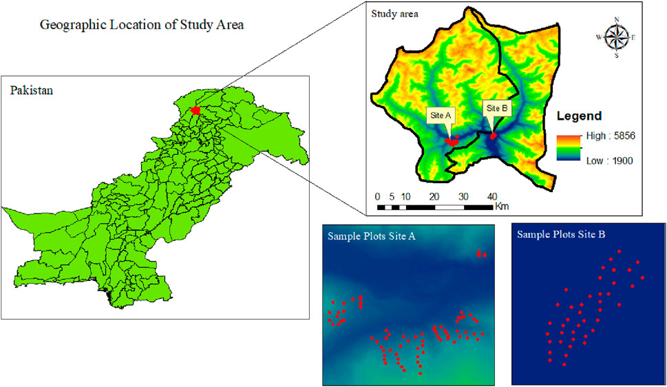
Figure 1. Map of the study area.

Inventory data

To collect the field inventory data for biomass modeling, the survey was conducted in July–August 2022. We selected a representative mountain from all the surrounding forested mountains having most of the major ecological, edaphic, and topographical features in common. We divided the dry temperate forest zone into site A and site B, where site A represents the Usho Forest and site B represents the Utror Forest. The area maps, topographic sheets, and growing stock data were obtained from the respective forest department office and available literature. We established 120 sample plots of (20 × 20 m) 400 m. A total area of 16,000 m (1.6 ha) was sampled at each altitudinal zone to analyze the composition and structure of the trees. Furthermore, with an area of (1 m × 1 m), 40 quadrates on each altitudinal zone in every sampled plot were taken to determine the biodiversity of herbs and shrubs. A geographic positioning system (GPS) was used to record the coordinates of each plot. In each plot, tree diameter (cm) and height (m), along with stem density, were measured. The tree diameter (cm) in each sample plot was measured by using a calibrated diameter tape at the breast height of trees. The standard diameter at breast height (DBH) was taken 4.5 feet above the ground from the uphill side. By dividing the circumference of trees by Pi (3.14), the circumference of the trees was converted into a diameter. Stem density is the number of trees per area. The stem density in each plot was calculated by counting the number of trees. The vertical distance between the highest tip of the tree and the base of the tree was taken as the tree height. Tree heights were measured by using the Haga altimeter. The total sample plots (120) were randomly split into a ratio of 80:20, where 80% (96 sample plots) were used for training the model and 20% (24 sample plots) were used for validation of the model (Table 1).

Table 1

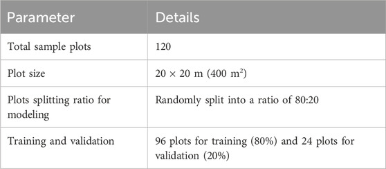
Table 1. Details of the sample plots surveyed.

Table 2

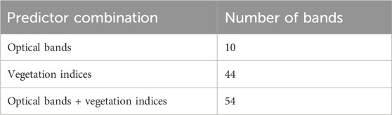
Table 2. Predictor combinations.

Digital elevation data

In this study, the SRTM digital elevation model (DEM) data were used to estimate the altitudinal gradients. The DEM was utilized to estimate the slope and aspect of the study area. Based on the natural break classification method, the elevation was classified into different ranges with an interval of 200 m in site A and site B. The obtained elevation ranges in site A were E1 = 2,009–2,061 m, E2 = 2,061–2,078 m, and E3 = 2,078–2,129 m and in site B, E1 = 2,200–2,400 m, E2 = 2,401–2,600 m, E3 = 2,601–2,800 m, and E4 = 2,801–3,000 m. Furthermore, the slope ranges were also classified in both sites; in site A, four slope ranges were calculated (S1 = 0.001–3.86; S2 = 3.86–7.36; S3 = 7.36–18.63; and S4 = 18.63–35.20), and for site B, four slope ranges were obtained (S1 = 4.9–19.2; S2 = 19.2–26.85; S3 = 26.85–34.16; and S4 = 34.16–48.95). In both sites, the different aspect ranges were checked (flat, north, northeast, east, southeast, south, southwest, west, and northwest).

Sentinel-2 data

In this study, the freely available high-resolution Sentinel-2 (S2) Level-2A product acquired on 16 October 2022 coincides with the survey month used. The S2 dataset was downloaded from the Copernicus Open Access Hub website (https://scihub.copernicus.eu/dhus). Sentinel-2 allows vegetation monitoring on regional and global scales at various spatial resolutions (10, 20, and 60 m) with a revisit frequency of 5 days and 12 spectral bands. There are four visible and near-infrared (NIR) bands with a spatial resolution of 10 m, six red-edge and short-wave infrared bands with a spatial resolution of 20 m, and two atmospheric bands with a spatial resolution of 60 m (Askar et al., 2018).

The Sentinel-2 Level-2 product underwent atmospheric correction and radiometric calibration, and to avoid the influence of cloud coverage on biomass modeling, images with a cloud coverage of less than 10% were selected for analysis. Band 1 (coastal aerosol), band 9 (water vapor), and band 10 (cirrus) were excluded and not considered in this research. The bands with spatial resolutions of 20 m were resampled to 10 m to ensure that all bands were in the same spatial resolution with aligned pixels.

Vegetation indexes

Based on prior biomass modeling research, 21 widely used vegetation indices were calculated using SNAP software. As Sentinel-2 has two NIR bands, the vegetation indices utilizing the NIR band were estimated with each NIR band separately. For example, the NDVI utilizes RED and NIR bands; therefore, one was calculated using NIR band 8 and another with NIR band 8a. In this way, the total number of vegetation indices reached 44, and the details of each index are given in Table 3.

Table 3

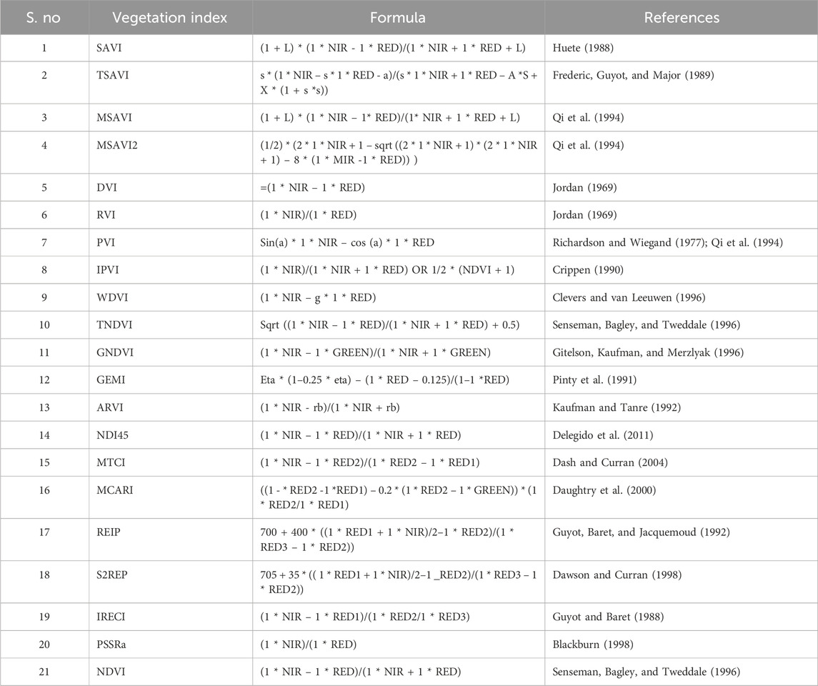
Table 3. Vegetation index compendium.

Extraction of remote sensing parameters from a field plot

Three different predictors were used in this study for biomass modeling. These predictors were developed from different kinds of spectral information, i.e., spectral bands only, vegetation indices only, and a combination of both (Table 2). First, the center coordinates of each plot were generated and used to extract the representative pixel of each predictor. Finally, these predictor features were used to train the RF model.

Random forest regression for AGB prediction

Mostly AGB from satellite images was predicted using regression models. In this study, to obtain the most suitable model for AGB modeling by comparative analysis, we adopted a machine learning random forest regression model (Breiman, 2001). RF has been applied extensively as a classification algorithm and for time-series forecasting in large-scale regression-based applications (Liaw and Wiener, 2002).

In the RF algorithms, a bootstrap sample of the training data is chosen, 80% of the training dataset is chosen randomly to build a decision tree, and the remaining part of the training dataset is used for estimating the out-of-bag error of each tree (Belgiu and Drăgu, 2016). At each node of the tree, a small sample of explanatory variables is chosen randomly to determine the best split. The coefficient of determination (R²) and the root mean square error (RMSE) were used to evaluate the model performance.

Validation of model outcomes

In this study, a 10-fold cross-validation approach, which was suggested by Tyralis, Papacharalampous, and Tantanee (2019), was performed to validate the performance of the RF regression model. Two error measurements, namely, R² and RMSE, were used to evaluate the performance of the RF model. In general, a higher R² value and lower RMSE values indicate a better estimation performance of the model (Equations 1, 2, 3) (Eckert, 2012).

RMSE:

$RMSE=\sqrt{\frac{{\displaystyle \sum _{i=1}^n}{\left(O_{\text{obs},i}-P_{\text{model},i}\right)}^2}{n}}.(1)$

Pearson’s coefficient R²:

$r=\frac{{\displaystyle \sum _{i=1}^n}\left(O_i-\overline{O}\right)\left(P_i-\overline{P}\right)}{\sqrt{{\displaystyle \sum _{i=1}^n}{\left(O_i-\overline{O}\right)}^2}\sqrt{{\displaystyle \sum _{i=1}^n}{\left(P_i-\overline{P}\right)}^2}}.(2)$

Mean absolute error (MAE) coefficient:

$MAE=\frac{1}{n}\times {\displaystyle \sum _{i=1}^n}\left|O_i-P_i\right|,(3)$

where O and P represent observed and predicted values, respectively.

Results and discussion

Biomass prediction in the study area

Utilizing vegetation indices, the maximum predicted AGB was 391 (Mg/ha), and the minimum predicted AGB was 131 (Mg/ha). Similarly, a combination of each high predicted biomass was 389 (Mg/ha). The lower predicted AGB was 116 (Mg/ha). However, the northern and western parts of site A were at higher altitudes, where the forest was less dense and less productive, and the biomass in the region was found to range from 150 to 286, 163 to 337, and 145 to 290 (Mg/ha) using spectral bands, vegetation indices, and a combination of both, respectively. Similarly, the northern and western parts of site B are at lower latitudes, despite the thinner forest of mixed species, so primarily, the biomass was found to range between 99.5 and 376, 131 and 391, and 116 and 389 (Mg/ha) using spectral bands, vegetation indices, and a combination of both, respectively in Figures 2A, B.

Figure 2

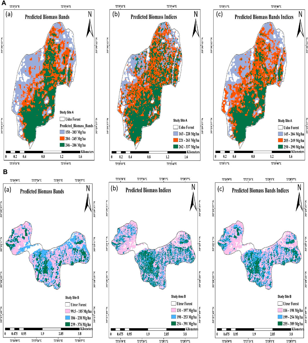
Figure 2. (A) Spatial AGB prediction map using Sentinel-2 data on (a) bands, (b) indices, and (c) bands and indices in site A, Usho Forest. (B) Spatial AGB prediction map using Sentinel-2 data on (a) bands, (b) indices, and (c) bands and indices in site B, Utror Forest.

Model validation

The random forest regression was used in both sites A and B for biomass prediction using the data on 120 sample plots. Based on the proportion of predictors explained by the model, the RF algorithm, using input variables of n = 10 for bands, n = 44 for vegetation indices, and n = 54 for the combination of both bands and indices, showed different levels of predictive performance. In site A R², RMSE, and MAE for the spectral bands were 0.83, 29.88, and 22.34, respectively, while for the vegetation indices, they were 0.74, 43.36, and 28.30, respectively. Similarly, R², RMSE, and MAE for the combination of bands and vegetation indices were 0.79, 30.71, and 21.86, respectively. In site B, the R², RMSE, and MAE for the spectral bands were 0.75, 53.11, and 34.47, respectively; for the vegetation indices, they were 0.83, 46.15, and 33.30, respectively, and for a combination of both, they were 0.82, 46.47, and 31.67, respectively. The scatterplots between the predicted and observed biomass values for both study sites using three combinations of predictors are shown in Figures 3A,B.

Figure 3

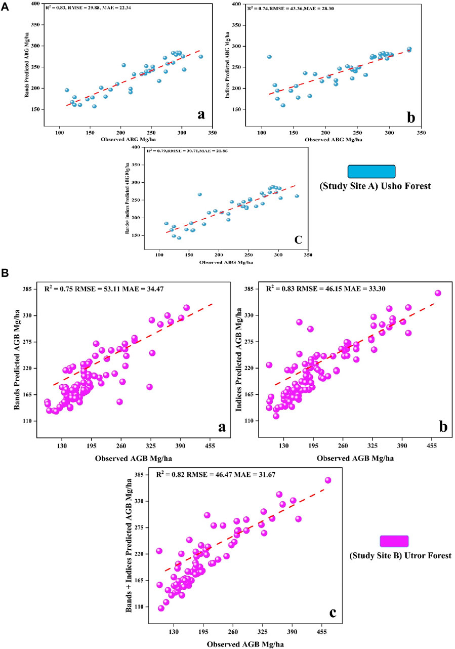
Figure 3. (A) (a) observed AGB and band-predicted AGB Mg/ha; (b) observed AGB and index-predicted AGB Mg/ha, and (c) shows the observed AGB and band + index-predicted AGB Mg/ha, in site A. (B) (a) observed AGB and band-predicted AGB Mg/ha, (b) observed AGB and index-predicted AGB Mg/ha, and (c) observed AGB and band + index-predicted AGB Mg/ha, in site B.

Biomass variation along altitudinal gradients

Elevation effect on predicted biomass

In site A, the predicted biomass using bands only was 237.89, 225.91, and 217.25 (Mg/ha) for E1, E2, and E3, respectively. The predicted biomass using vegetation indices was 255.44, 250.30, and 240.67 (Mg/ha) and a combination of bands and indices was 244.24, 231.47, and 214.11 (Mg/ha) for E1, E2, and E3, respectively. In site B, the elevation was divided into four ranges: E1, E2, E3, and E4. The predicted biomass using bands was 200.82, 195.60, 205.88, and 198.36 (Mg/ha) in E1, E2, E3, and E4, respectively. However, the predicted biomass using vegetation indices was 199.46, 214.41, 223.12, and 220.42, and using a combination of bands and vegetation indices, it was 188.39, 209.76, 221.79, and 221.79 in E1, E2, E3, and E4 respectively. The best results obtained in different elevation ranges for site A were for E1 for the vegetation indices, which shows that high predicted biomass for site B was E1 for the spectral bands, as shown in Figures 4A,B. Furthermore, the correlation between the predicted biomass and elevation ranges showed that the biomass is highly correlated with elevation range E3, which is 0.91 in the predicted biomass band (PBB) in site A, while in site B, the high correlation was found in E2, which is 0.87 in PBB Figure 4C.

Figure 4

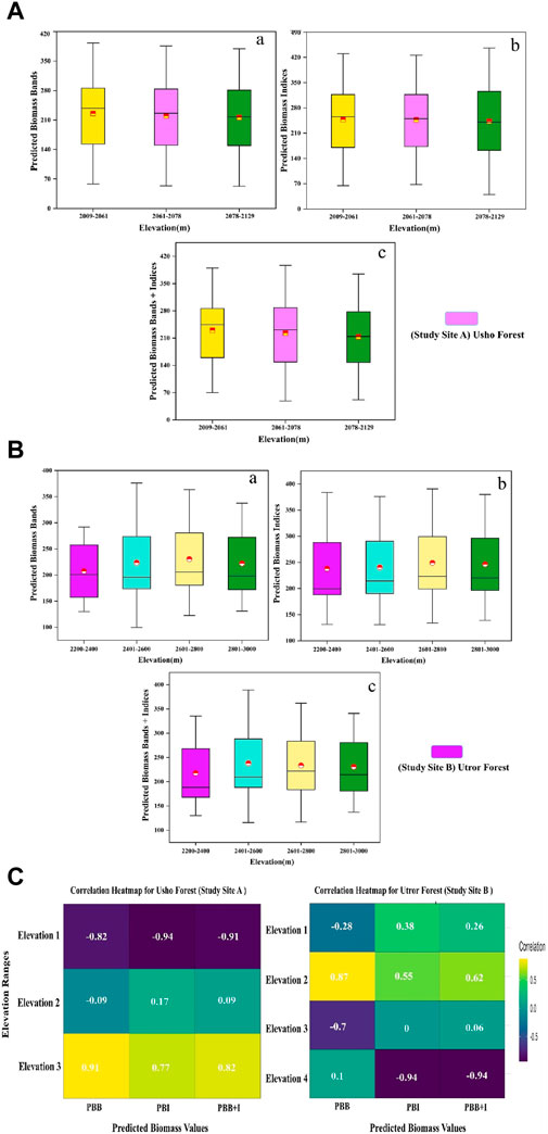
Figure 4. (A) (a) effect of three elevations (E1, E2, and E3) on predicted AGB Mg/ha of bands, (b) effect of three elevations on predicted AGB Mg/ha of indices, and (c) effect of three elevations on predicted AGB Mg/ha bands + indices of site A. (B) (a) effect of four elevations (E1, E2, E3, and E4) on predicted AGB Mg/ha of bands; (b) effect of four elevations on predicted AGB Mg/ha of indices, and (c) effect of four elevations on predicted AGB Mg/ha bands + indices of site B. (C) PBB is the predicted biomass band; PBI is the predicted biomass index; and PBB + +I is the predicted biomass bands and indices.

Slope effect on predicted biomass

The predicted biomass in site A using bands was 230.20, 226.17, 230.11, and 219.73 (Mg/ha); using vegetation indices was 251.44, 247.41, 252.92, and 250.53; and using a combination of both was 233.34, 226.40, 229.24, and 233.64 (Mg/ha) for slope ranges S1, S2, S3, and S4, respectively. The best biomass was predicted using a combination of bands and vegetation indices in the slope S4 range at site A. Similarly, the biomass predicted for the same slope ranges in site B using bands was 201.56, 206.08, 196.22, and 196.67 (Mg/ha); using vegetation indices was 210.87, 219.49, 219.75, and 220.60 (Mg/ha); and using both spectral bands and vegetation indices was 208.58, 217.02, 213.91, and 215.65 (Mg/ha); the best results are shown in the vegetation indices within the slope S4 range, as shown in Figures 5A,B. In addition, the analysis revealed a strong correlation between the expected biomass and slope range in both site A and site B. Specifically, in site A, the biomass shows a significant correlation with slope range S1, with a correlation coefficient of 0.67 in the PBB + I model. On the other hand, in site B, the highest correlation was observed with slope range S4, with a correlation level of 0.49 in the PBB simulation, as shown in Figure 6A).

Figure 5

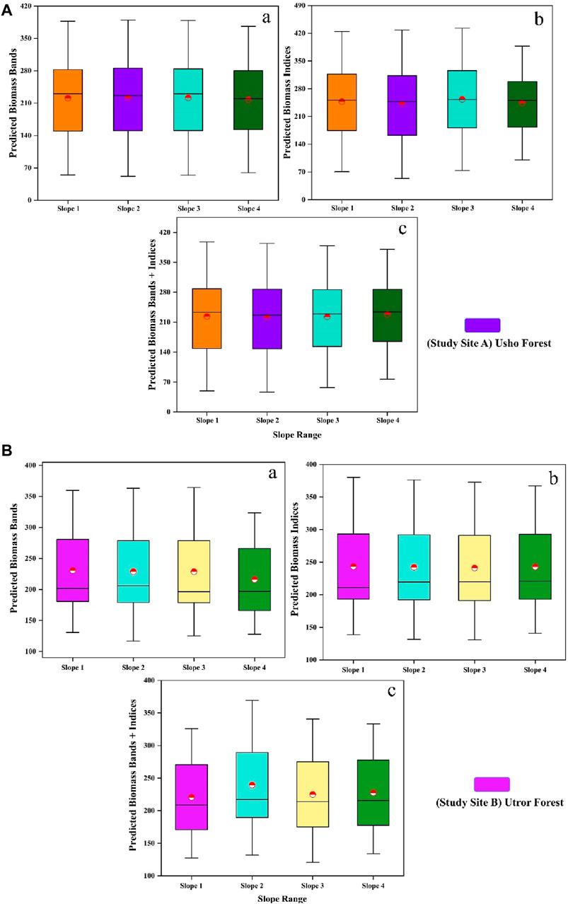
Figure 5. (A) (a) effect of four different slopes (S1, S2, S3, and S4) on predicted AGB Mg/ha of bands; (b) effect of four different slopes on predicted AGB Mg/ha of indices; and (c) effect of four different slopes on predicted AGB Mg/ha of bands and indices of site A. (B) (a) effect of four different slopes (S1, S2, S3, and S4) on predicted AGB Mg/ha of bands; (b) effect of four different slopes on predicted AGB Mg/ha of indices; and (c) effect of four different slopes on predicted AGB Mg/ha of bands and indices of site B.

Figure 6

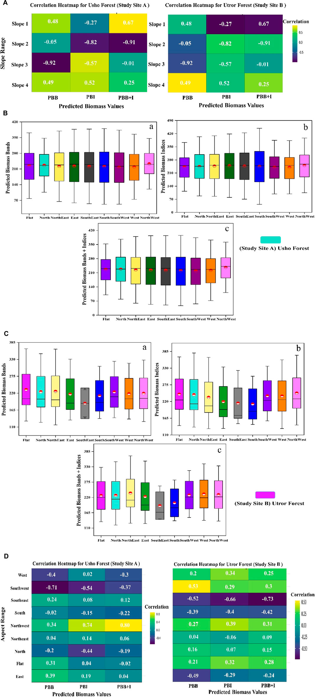
Figure 6. (A) PBB is the predicted biomass band, PBI is the predicted biomass index, and PBB + I is the predicted biomass band and index. (B) Effect of aspect on the predicted biomass, where (a) shows the effect of different aspects on predicted AGB Mg/ha of bands; (b) shows the effect of four different aspects on predicted AGB Mg/ha of indices; and (c) shows the effect of different aspects on predicted AGB Mg/ha of bands and indices of site A. (C) Effect of aspect on predicted biomass where (a) shows the effect of different aspects on predicted AGB Mg/ha of bands; (b) shows the effect of four different aspects on predicted AGB Mg/ha of indices, and (c) shows the effect of different aspects on predicted AGB Mg/ha of bands and indices of site B. (D) PBB is the predicted biomass band, PBI is the predicted biomass indexes, and PBB + I is the predicted biomass band and index.

Effect of aspect on the predicted biomass

To further investigate the spatial distribution of biomass, different slope aspects for both sites A and B were estimated, including flat, north, northeast, east, southeast, south, southwest, west, and northwest. In site A, the highest biomass distribution using bands only was at east followed by northwest, flat area, southeast, northeast, south, north, west, and southwest. Similarly, using vegetation indices, the highest predicted biomass was at northwest and lowest at southwest, while using a combination of bands and indices, the highest was recorded in the northwest and lowest in southwest. Furthermore, in site B, the predicted biomass utilizing bands was 201.89, 200.81, 198.51, 187.68, 187.05, 189.71, 208.40, 201.74, and 203.09 (Mg/ha) for flat, north, northeast, east, southeast, south, southwest, west, and northwest, respectively. Similarly, using vegetation indices, the predicted biomass was 225.11, 212.42, 205.78, 193.80, 174.53, 187.86, 223.64, 226.13, and 228.70 (Mg/ha), and using a combination of bands and indices, it was 220.16, 213.56, 210.37, 192.69, 166.70, 183.01, 221.29, 218.70, and 221.92 (Mg/ha) in the flat, north, northeast, east, southeast, south, southwest, west, and northwest aspects, respectively. The overall results show that the west aspect has good predicted biomass in the predictor combination, spectral bands, indices, and combination of both, respectively, as shown in Figures 6B,C. The assessment indicated a strong correlation between aspects and predicted biomass, using both bands and indices. Specifically, the aspect ranges in the northwest of site A showed a high correlation of 0.80 with the predicted biomass when using bands and indices. In site B, the southwest aspect ranges showed a correlation of 0.53 with the predicted biomass in the PBB (Figure 6D).

Variable importance in AGB modeling

In total, 54 variables were used in AGB modeling in the study areas, i.e., 10 spectral bands and 44 vegetation indices. Random forest has the capability to evaluate the variable importance during modeling. The variable importance of all the spectral bands and vegetation indices for each study site (A and B) was evaluated separately, as shown in Figure 7. In site A, the top 10 important variables were ARVI8A, NDI45, B12, S2REP, GEMI, PVI8A, REIP8A, S2REIP8, MTCI8A, and IRECI8A. Similarly, for site B, the highly important variables were B12 and B11, followed by TSAVI8, ARVI8A, NDVI45, ARVI8, NDVI8A, B4, TNDVI8A, and TNDVI8. Furthermore, due to differences in the geography and physical structure of forests in sites A and B, the variables’ importance is not same.

Figure 7

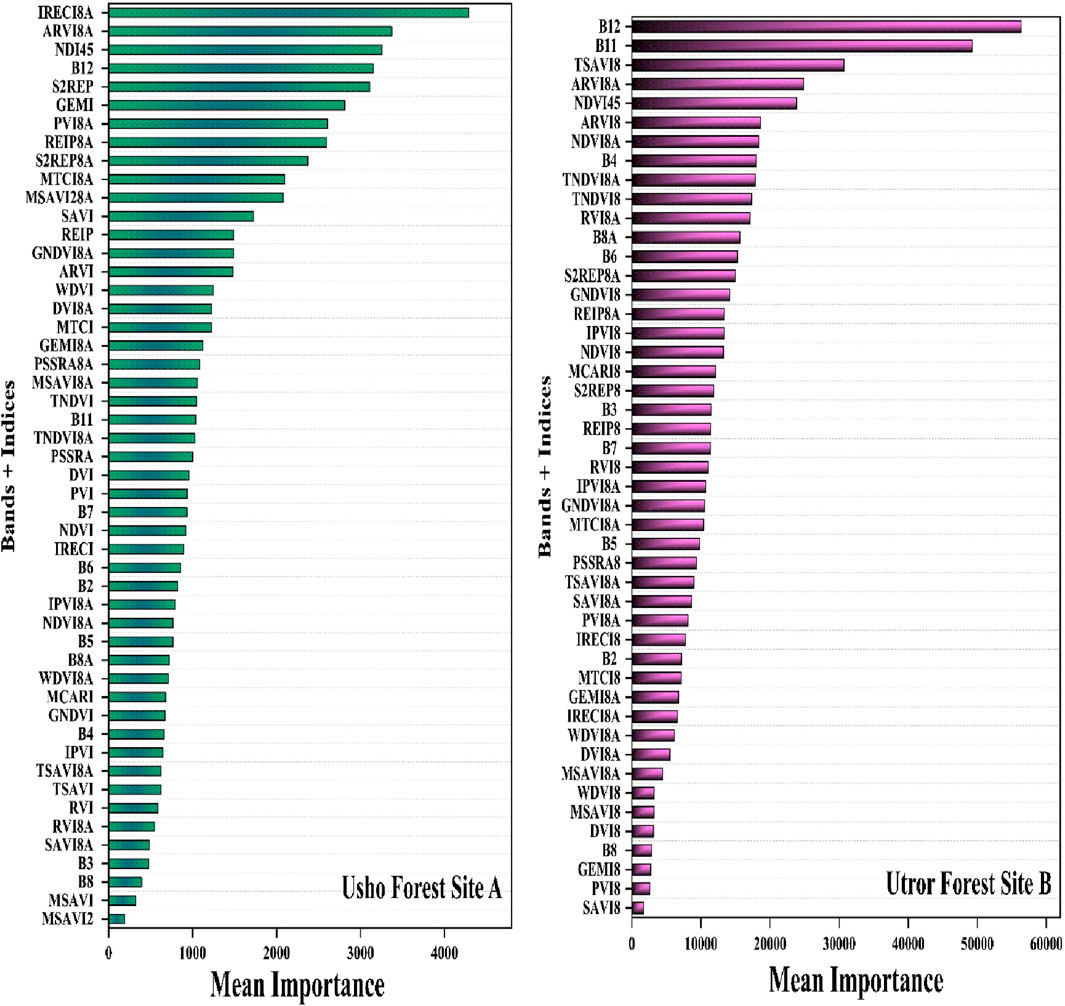
Figure 7. Importance of variables of bands and indices of sites A and B.

Discussion

Biomass distribution in the study area

The biomass prediction in site A (Usho Forest) and site B (Utror Forest), using ground biomass and the random forest regression model, aligns with contemporary research emphasizing the significance of spatial and environmental factors in comprehending forest biomass distribution. Previous studies (Qadeer et al., 2024) carried out forest biomass estimation through remote sensing and machine learning techniques, corroborating the efficacy of random forest models in capturing intricate relationships within diverse forest ecosystems. The identified patterns of diminished forest density at higher altitudes in site A and the influence of latitude and forest composition on biomass in site B resonate with the findings obtained by Thapa et al. (2023), who explored biomass variations in subtropical forests, underscoring the role of topographical and climatic factors. The study methodology, integrating advanced modeling techniques and ground data, contributes to the evolving landscape of forest biomass research, advancing our understanding of the intricate interplay between environmental variables and biomass patterns in different forest ecosystems (Wijaya et al., 2013; Ploton et al., 2017; Guanglong et al., 2019). The resulted AGB maps exhibit spatial distributions, effectively masking non-forest areas. In site A, the study discerns reduced forest density and productivity at higher altitudes in the northern and western regions, resulting in biomass ranges of 150–203, 163–220, and 145–204 Mg/ha. Conversely, site B, characterized by lower latitudes and a mix of thinner forests, displays biomass ranges of 99.5–185, 131–197, and 116–198 Mg/ha. This comprehensive approach significantly contributes to current research efforts aimed at unraveling the complexities of forest biomass dynamics in varied environmental contexts.

In our study of biomass distribution in site A (Usho Forest) and site B (Utror Forest), we employed ground biomass data and random forest regression models, reflecting recent advancements in forest biomass estimation. Random forest regression models achieved high accuracy in estimating the forest biomass in northern China, using Landsat 9 imagery, lending credibility to our approach (Jiang et al., 2022). In site A, we observed reduced forest density at higher altitudes, resulting in biomass ranges of 150–203, 163–220, and 145–204 Mg/ha. This finding is consistent with that obtained by He et al. (2022), who quantified the effects of stand and climate variables on biomass in larch plantations in China, affirming the influence of altitude and environmental factors on biomass. Conversely, site B, with lower latitudes and a mix of thinner forests, displayed biomass ranges of 99.5–185, 131–197, and 116–198 Mg/ha. This pattern aligns with the findings obtained by Liu et al. (2022), who explored biomass estimation in different forest types, emphasizing the impact of forest composition on biomass distribution. The effectiveness of recent studies such as that by Li et al. (2022), which combined data from multiple sensors to predict forest above-ground biomass with increased accuracy and robustness, was replicated by our approach to AGB mapping, which effectively obscured non-forest areas. Li et al. (2023) investigated the influence of forest composition on biomass distribution by examining biomass estimation in various forest types.

Random forest for biomass modeling

The random forest regression model yielded promising results. As mentioned above, Breiman (2001) invented the RF machine learning method, which is a set of binary rule-based decisions that determine how an input relates to its dependent variable. One of the primary benefits of RF is its ability to effectively depict complicated relationships between independent factors and dependent variables, which are frequently encountered when complex ecological systems and environmental variables are added (Fu et al., 2017). In site A, the model demonstrated notable R² values of 0.83 for spectral bands, 0.74 for vegetation indices, and 0.79 for the combination of bands and indices. Correspondingly, the RMSE values were 29.99, 34.36, and 30.71, while the MAE values stood at 22.34, 28.30, and 21.86 for bands, indices, and a combination of both, respectively. In site B, the model performance was robust, evidenced by R² values of 0.75 (spectral bands), 0.83 (vegetation indices), and 0.82 (bands and indices). The associated RMSE values were 53.11, 46.15, and 46.47, and the MAE values were 34.47, 33.30, and 31.67, respectively. These outcomes align with those of contemporary research on the efficacy of the random forest algorithm in biomass prediction, as indicated by studies such as those by Pham et al. (2020) and Rasel et al. (2021). The scatterplots depicting the agreement between predicted and observed biomass values further reinforce the robustness and practical utility of the model.

Biomass variation along the altitudinal gradient

Effective forest biomass estimation through remote sensing relies on meticulous model selection and application, directly shaping the accuracy and minimizing the uncertainty in estimations. The precision of biomass assessments hinges on the strategic use of models, emphasizing their critical role in obtaining reliable and consistent outcomes (Lu, 2006; Shettles et al., 2015). The predicted biomass variations along altitudinal gradients in site A (elevation ranges E1, E2, and E3) revealed distinct patterns for spectral bands, vegetation indices, and their combination. For instance, in E1, the predicted biomass for bands was 237.89 Mg/ha, vegetation indices showed 255.44 Mg/ha, and the combination yielded 244.24 Mg/ha. In site B (E1, E2, E3, and E4), the predicted biomass ranged from 200.82 Mg/ha to 198.36 Mg/ha for bands and 199.46 Mg/ha to 220.42 Mg/ha for vegetation indices. Optimal results were observed in E1 for site A, emphasizing the importance of vegetation indices, while for site B, E1 exhibited superior results for spectral bands (Pham et al., 2020). A similar trend was observed in the slope effect analysis, where site A S4 showed the best biomass predictions for both bands (233.64 Mg/ha) and vegetation indices (250.53 Mg/ha). In site B, the highest biomass for the slope effect occurred in vegetation indices (215.65 Mg/ha) in S4. Furthermore, the analysis of aspect on predicted biomass demonstrated varying results across different aspects for both sites. Notably, Site-A's flat aspect exhibited the highest predicted biomass for bands (230.41 Mg/ha) and vegetation indices (249.83 Mg/ha). In site B, the west aspect showed the best results for spectral bands (203.09 Mg/ha), vegetation indices (228.70 Mg/ha), and their combination (221.92 Mg/ha). In our study, the meticulous validation of biomass prediction models for site A and site B forests, using the RF algorithm with a dataset of 120 plot samples and a diverse set of input variables, yielded promising results. The invention of the RF machine learning method by Breiman (2001) has been a foundational development in this field. The ability of RF to effectively depict complex relationships between independent and dependent variables is especially beneficial in ecological systems.

In site A, the model demonstrated strong R² values (0.83 for spectral bands, 0.74 for vegetation indices, and 0.79 for the combination), with corresponding RMSE values of 29.99, 34.36, and 30.71 and MAE values of 22.34, 28.30, and 21.86, respectively. In site B, the model showed robust performance, with R² values of 0.75, 0.83, and 0.82; RMSE values of 53.11, 46.15, and 46.47; and MAE values of 34.47, 33.30, and 31.67. These outcomes align with those of contemporary research, such as the study by Fassnacht et al. (2014), who noted the high performance of RF in biomass prediction using LiDAR data. Additionally, Esteban et al. (2019) highlighted the increased precision of RF in forest volume and biomass predictions using remotely sensed data.

However, the altitudinal gradients significantly influence biomass distribution; optimal elevation ranges for AGB harvest are 2,009–2,061 m for site A and 2,601–2,800 m for site B. Similarly, among different aspects, the highest significance levels observed are northwest and southwest aspects in sites A and B, respectively.

Furthermore, the scatterplots depicting the agreement between the predicted and observed biomass values reinforce the robustness and practical utility of the RF model. This is supported by Bilous et al. (2017), who reported high accuracy in estimating forest stock volume and live biomass using RF. The efficacy of RF in handling complex correlations between variables is also evidenced in the study by Ullah et al. (2021), demonstrating the suitability of RF in bio-oil yield prediction.

Variable importance in AGB modeling

The importance of variables in AGB modeling was assessed using the random forest algorithm. In site A, the high-ranked variables were ARVI8A, NDI45, and B12, while in site B, the high-ranked variables include B11, TSAVI8, and ARVI8A. Previous studies (Crippen, 1990; Moradi et al., 2022) also highlight that variable ARVI8A is a key contributor in biomass modeling. Furthermore, due to differences in the physical structure and density of forests in site A and site B, the variables’ ranking in both sites was not same. These differences in the variables’ ranking can be attributed to the fact that a forest with different ages, structures, and densities has different spectral responses. In the assessment of variable importance for AGB modeling using the random forest algorithm, key contributors such as ARVI8A, NDI45, and B12 in site A and B11, TSAVI8, and ARVI8A in site B were identified. This highlights the importance of considering factors like elevation, slope, aspect, and specific spectral variables in refining biomass predictions for diverse forest ecosystems. The high importance of ARVI8A, NDI45, and B12 in site A aligns with the findings obtained by Lourenço et al. (2021), who identified vegetation indices and spectral bands as the top variables for estimating tree AGB in Mediterranean agroforestry systems. In contrast, the variable rankings in site B reflect the different spectral responses due to variations in forest age, structure, and density.

Conclusion

This work utilized Sentinel-2 data and a random forest regression model to accurately estimate and map the AGB in the difficult terrain of the Usho and Utror forests in northern Pakistan. The study utilized ground biomass data from specific research locations in hilly areas to uncover detailed spatial patterns of AGB. Non-forest areas were excluded from the analysis using an NDVI threshold. The investigation, which included the examination of spectral bands, vegetation indexes, and machine learning approaches, yielded detailed and subtle insights into the fluctuations in the AGB. Altitudinal gradients were found to be important factors affecting the distribution of biomass. This conclusion was further supported by slope analysis. The western features consistently exhibited the greatest biomass, and the analysis of variable importance showed the main predictors. The comprehensive methodology greatly enhances our comprehension of the distribution of the AGB in arid temperate ecosystems, providing valuable implications for the implementation of sustainable forest management and environmental preservation in the area. The comprehensive methodology of the study and precise quantitative analysis bolster its scientific legitimacy.

Data availability statement

The raw data supporting the conclusion of this article will be made available by the authors, without undue reservation.

Author contributions

BM: conceptualization, formal analysis, software, supervision, validation, writing–original draft. AR: data curation, software, validation, writing–review and editing. FM: writing–review and editing, data curation, investigation, validation. YQ: supervision, funding acquisition, validation, writing–review and editing. JZ: writing–review and editing, funding acquisition, methodology, resources, supervision.

Funding

The author(s) declare that financial support was received for the research, authorship, and/or publication of this article. Effects of spatial variability and biological factors on trunk respiration of Larix principis-rupprechtii and its internal mechanism: Grant Number: 31870387.

Conflict of interest

The authors declare that the research was conducted in the absence of any commercial or financial relationships that could be construed as a potential conflict of interest.

The author(s) declared that they were an editorial board member of Frontiers, at the time of submission. This had no impact on the peer review process and the final decision.

Publisher’s note

All claims expressed in this article are solely those of the authors and do not necessarily represent those of their affiliated organizations, or those of the publisher, the editors, and the reviewers. Any product that may be evaluated in this article, or claim that may be made by its manufacturer, is not guaranteed or endorsed by the publisher.

References

Ahmad, A., Nizami, S. M., Marwat, K. B., and Muhammad, J. (2015). Annual accumulation of carbon in the coniferous forest of dir kohistan: an inventorybased estimate. Pak. J. Bot. 47 (SI), 115–118.

Google Scholar

Askar, N. N., Phairuang, W., Wicaksono, P., and Sayektiningsih, T. (2018). Estimating aboveground biomass on private forest using sentinel-2 imagery. J. Sensors 2018, 1–11. doi:10.1155/2018/6745629

CrossRef Full Text | Google Scholar

Badshah, M. T., Ahmad, A., Muneer, M. A., Rehman, A. U., Wang, J., Khan, M. A., et al. (2020). Evaluation of the forest structure, diversity and biomass carbon potential in the Southwest region of guangxi, China. Appl. Ecol. Environ. Res. 18, 447–467. doi:10.15666/aeer/1801_447467

CrossRef Full Text | Google Scholar

Badshah, M. T., Hussain, K., Rehman, A.Ur, Mehmood, K., Muhammad, B., Wiarta, R., et al. (2024). The role of random forest and Markov chain models in understanding metropolitan urban growth trajectory. Front. For. Glob. Change 7 (March), 1–17. doi:10.3389/ffgc.2024.1345047

CrossRef Full Text | Google Scholar

Beer, C., Reichstein, M., Tomelleri, E., Ciais, P., Jung, M., Carvalhais, N., et al. (2010). Terrestrial gross carbon dioxide uptake: global distribution and covariation with climate. Science 329 (5993), 834–838. doi:10.1126/science.1184984

PubMed Abstract | CrossRef Full Text | Google Scholar

Belgiu, M., and Drăgu, L. (2016). Random forest in remote sensing: a review of applications and future directions. ISPRS J. Photogrammetry Remote Sens. 114, 24–31. doi:10.1016/j.isprsjprs.2016.01.011

CrossRef Full Text | Google Scholar

Bilous, A., Myroniuk, V., Holiaka, D., Bilous, S., See, L., and Schepaschenko, D. (2017). Mapping growing stock volume and forest live biomass: a case study of the polissya region of Ukraine. Environ. Res. Lett. 12 (10), 105001. doi:10.1088/1748-9326/aa8352

CrossRef Full Text | Google Scholar

Blackburn, G. A. (1998). Quantifying chlorophylls and caroteniods at leaf and canopy scales: an evaluation of some hyperspectral approaches. Remote Sens. Environ. 66 (3), 273–285. doi:10.1016/s0034-4257(98)00059-5

CrossRef Full Text | Google Scholar

Breiman, L. (2001). Random forests. Mach. Learn. 45, 5–32. doi:10.1023/a:1010933404324

CrossRef Full Text | Google Scholar

Clevers, J. G. P. W., and van Leeuwen, H. J. C. (1996). Combined use of optical and microwave remote sensing data for crop growth monitoring. Remote Sens. Environ. 56 (1), 42–51. doi:10.1016/0034-4257(95)00227-8

CrossRef Full Text | Google Scholar

Crippen, R. E. (1990). Calculating the vegetation index faster. Remote Sens. Environ. 34 (1), 71–73. doi:10.1016/0034-4257(90)90085-z

CrossRef Full Text | Google Scholar

Dash, J., and Curran, P. J. (2004). The MERIS terrestrial chlorophyll index. Int. J. Remote Sens. 25 (23), 5403–5413. doi:10.1080/0143116042000274015

CrossRef Full Text | Google Scholar

Daughtry, C. S. T., Walthall, C. L., Kim, M. S., de Colstoun, E. B., and McMurtrey, J. E. (2000). Estimating corn leaf chlorophyll concentration from leaf and canopy reflectance. Remote Sens. Environ. 74 (2), 229–239. doi:10.1016/S0034-4257(00)00113-9

CrossRef Full Text | Google Scholar

Dawson, T. P., and Curran, P. J. (1998). Technical note A new technique for interpolating the reflectance red edge position. Int. J. Remote Sens. 19, 2133–2139. doi:10.1080/014311698214910

CrossRef Full Text | Google Scholar

Delegido, J., Verrelst, J., Alonso, L., and Moreno, J. (2011). Evaluation of sentinel-2 red-edge bands for empirical estimation of green LAI and chlorophyll content. Sensors Basel, Switz. 11 (December), 7063–7081. doi:10.3390/s110707063

PubMed Abstract | CrossRef Full Text | Google Scholar

Eckert, S. (2012). Improved forest biomass and carbon estimations using texture measures from WorldView-2 satellite data. Remote Sens. 4 (4), 810–829. doi:10.3390/rs4040810

CrossRef Full Text | Google Scholar

Esteban, J., McRoberts, R. E., Fernández-Landa, A., Tomé, J. L., and Nӕsset, E. (2019). Estimating forest volume and biomass and their changes using random forests and remotely sensed data. Remote Sens. 11 (16), 1944. doi:10.3390/rs11161944

CrossRef Full Text | Google Scholar

Fassnacht, F. E., Hartig, F., Latifi, H., Berger, C., Hernández, J., Corvalán, P., et al. (2014). Importance of sample size, data type and prediction method for remote sensing-based estimations of aboveground forest biomass. Remote Sens. Environ. 154, 102–114. doi:10.1016/j.rse.2014.07.028

CrossRef Full Text | Google Scholar

Frampton, W. J., Dash, J., Watmough, G., and Milton, E. J. (2013). Evaluating the capabilities of sentinel-2 for quantitative estimation of biophysical variables in vegetation. ISPRS J. Photogrammetry Remote Sens. 82, 83–92. doi:10.1016/j.isprsjprs.2013.04.007

CrossRef Full Text | Google Scholar

Frederic, B., Guyot, G., and Major, D. (1989). “TSAVI: a vegetation index which minimizes soil brightness effects on lai and APAR estimation,” in 12th Canadian Symposium on Remote Sensing Geoscience and Remote Sensing Symposium, Vancouver, BC, Canada, 10-14 July 1989 (IEEE).

Google Scholar

Friedl, M., McGwire, K., and McIVer, D. (2001). “An overview of uncertainty in optical remotely sensed data for ecological applications,” in Spatial uncertainty in ecology (Springer), 258–283. doi:10.1007/978-1-4613-0209-4_12

CrossRef Full Text | Google Scholar

Fu, B., Wang, Y., Campbell, A., Li, Y., Zhang, B., Yin, S., et al. (2017). Comparison of object-based and pixel-based random forest algorithm for wetland vegetation mapping using high spatial resolution GF-1 and SAR data. Ecol. Indic. 73, 105–117. doi:10.1016/j.ecolind.2016.09.029

CrossRef Full Text | Google Scholar

Gitelson, A. A., Kaufman, Y. J., and Merzlyak, M. N. (1996). Use of a green channel in remote sensing of global vegetation from EOS-MODIS. Remote Sens. Environ. 58 (3), 289–298. doi:10.1016/s0034-4257(96)00072-7

CrossRef Full Text | Google Scholar

Guanglong, Ou, Li, C., Lv, Y., Wei, A., Xiong, H., Xu, H., et al. (2019). Improving aboveground biomass estimation of pinus densata forests in yunnan using Landsat 8 imagery by incorporating age dummy variable and method comparison. Remote Sens. 11 (March), 738. doi:10.3390/rs11070738

CrossRef Full Text | Google Scholar

Guyot, G., and Baret, F. (1988). Utilisation de La Haute Resolution Spectrale Pour Suivre l’etat Des Couverts Vegetaux. Spectr. Signatures Objects Remote Sens. 287, 279.

Google Scholar

Guyot, G., Baret, F., and Jacquemoud, S. (1992). Imaging spectroscopy for vegetation studies volume 2. Norwell, MA, USA: Kluwer Academic Publishers.

Google Scholar

Hall, F. G., Bergen, K., Blair, J. B., Dubayah, R., Houghton, R., George, H., et al. (2011). Characterizing 3D vegetation structure from space: mission requirements. Remote Sens. Environ. 115 (11), 2753–2775. doi:10.1016/j.rse.2011.01.024

CrossRef Full Text | Google Scholar

Hamayun, M., Khan, S. A., Young Sohn, E., and In-Jung, L. (2006). Folk medicinal knowledge and conservation status of some economically valued medicinal plants of District Swat, Pakistan. Lyonia 11 (2), 101–113.

Google Scholar

He, X., Lei, X., Zeng, W., Feng, L., Zhou, C., and Wu, B. (2022). Quantifying the effects of stand and climate variables on biomass of larch plantations using random forests and national forest inventory data in north and northeast China. Sustainability 14 (9), 5580. doi:10.3390/su14095580

CrossRef Full Text | Google Scholar

Huete, A. R. (1988). A soil-adjusted vegetation index (SAVI). Remote Sens. Environ. 25 (3), 295–309. doi:10.1016/0034-4257(88)90106-X

CrossRef Full Text | Google Scholar

Jiang, F., Sun, H., Chen, E., Wang, T., Cao, Y., and Liu, Q. (2022). Above-ground biomass estimation for coniferous forests in northern China using regression kriging and Landsat 9 images. Remote Sens. 14 (22), 5734. doi:10.3390/rs14225734

CrossRef Full Text | Google Scholar

Jordan, C. F. (1969). Derivation of leaf-area index from quality of light on the forest floor. Ecology 50 (4), 663–666. doi:10.2307/1936256

CrossRef Full Text | Google Scholar

Kaufman, Y. J., and Tanre, D. (1992). Atmospherically resistant vegetation index (ARVI) for EOS-MODIS. IEEE Trans. Geoscience Remote Sens. 30 (2), 261–270. doi:10.1109/36.134076

CrossRef Full Text | Google Scholar

Laurin, G. V., Chen, Qi, Lindsell, J. A., Coomes, D. A., Del Frate, F., Guerriero, L., et al. (2014). Above ground biomass estimation in an african tropical forest with lidar and hyperspectral data. ISPRS J. Photogrammetry Remote Sens. 89, 49–58. doi:10.1016/j.isprsjprs.2014.01.001

CrossRef Full Text | Google Scholar

Liaw, A., and Wiener, M. (2002). Classification and regression by RandomForest. R J. 2, 18–22.

Google Scholar

Li, Y., Li, M., and Wang, Y. (2022). Forest aboveground biomass estimation and response to climate change based on remote sensing data. Sustainability 14, 14222. doi:10.3390/su142114222

CrossRef Full Text | Google Scholar

Li, L., Zhou, B., Liu, Y., Wu, Y., Tang, J., Xu, W., et al. (2023). Reduction in uncertainty in forest aboveground biomass estimation using sentinel-2 images: a case study of pinus densata forests in Shangri-La City, China. Remote Sens. 15, 559. doi:10.3390/rs15030559

CrossRef Full Text | Google Scholar

Liu, C., Chen, D., Zou, C., Liu, S., Li, Hu, Liu, Z., et al. (2022). Modeling biomass for natural subtropical secondary forest using multi-source data and different regression models in huangfu mountain, China. Sustainability 14 (20), 13006. doi:10.3390/su142013006

CrossRef Full Text | Google Scholar

Lourenço, P., Godinho, S., Sousa, A., and Gonçalves, A. C. (2021). Estimating tree aboveground biomass using multispectral satellite-based data in mediterranean agroforestry system using random forest algorithm. Remote Sens. Appl. Soc. Environ. 23, 100560. doi:10.1016/j.rsase.2021.100560

CrossRef Full Text | Google Scholar

Lu, D. (2006). The potential and challenge of remote sensing-based biomass estimation. Int. J. Remote Sens. 27 (7), 1297–1328. doi:10.1080/01431160500486732

CrossRef Full Text | Google Scholar

Lu, D., Qi, C., Wang, G., Liu, L., Li, G., and Moran, E. (2016). A survey of remote sensing-based aboveground biomass estimation methods in forest ecosystems. Int. J. Digital Earth 9 (1), 63–105. doi:10.1080/17538947.2014.990526

CrossRef Full Text | Google Scholar

Lu, D., Qi, C., Wang, G., Moran, E., Batistella, M., Zhang, M., et al. (2012). Aboveground forest biomass estimation with Landsat and LiDAR data and uncertainty analysis of the estimates. Int. J. For. Res. 2012 (April), 1–16. doi:10.1155/2012/436537

CrossRef Full Text | Google Scholar

Maia, V. A., Rodrigo de Souza, C., de Aguiar-Campos, N., Fagundes, N. C. A., Santos, A. B. M., de Paula, G. G. P., et al. (2020). Interactions between climate and soil shape tree community assembly and above-ground woody biomass of tropical dry forests. For. Ecol. Manag. 474, 118348. doi:10.1016/j.foreco.2020.118348

CrossRef Full Text | Google Scholar

McRoberts, R. E., and Tomppo, E. O. (2007). Remote sensing support for national forest inventories. Remote Sens. Environ. 110 (4), 412–419. doi:10.1016/j.rse.2006.09.034

CrossRef Full Text | Google Scholar

Moradi, F., Ali, A. D., Rajab Pourrahmati, M., Deljouei, A., and Borz, S. A. (2022). Estimating aboveground biomass in dense hyrcanian forests by the use of sentinel-2 data. Forests 13 (1), 104. doi:10.3390/f13010104

CrossRef Full Text | Google Scholar

Peng, D., Zhang, H., Liu, L., Huang, W., Huete, A., Zhang, X., et al. (2019). Estimating the aboveground biomass for planted forests based on stand age and environmental variables. Remote Sens. 11 (September), 2270. doi:10.3390/rs11192270

CrossRef Full Text | Google Scholar

Pham, T. D., Yokoya, N., Xia, J., Thang, Ha, Le, N., Thu, T., et al. (2020). Comparison of machine learning methods for estimating mangrove above-ground biomass using multiple source remote sensing data in the red river delta biosphere reserve, vietnam. Remote Sens. 12 (April), 1334. doi:10.3390/rs12081334

CrossRef Full Text | Google Scholar

Pinty, B., Verstraete, M. M., Huete, A., Kerr, Y., and Sorooshian, S. (1991). GEMI: a non-linear index to monitoring global gegetation index (msavi). Remote Sens. Environ. 48, 119–126. doi:10.1016/0034-4257(94)90134-1

CrossRef Full Text | Google Scholar

Ploton, P., Barbier, N., Couteron, P., Antin, C. M., Ayyappan, N., Balachandran, N., et al. (2017). Toward a general tropical forest biomass prediction model from very high resolution optical satellite images. Remote Sens. Environ. 200, 140–153. doi:10.1016/j.rse.2017.08.001

CrossRef Full Text | Google Scholar

Qadeer, A., Shakir, M., Wang, Li, and Talha, S. M. (2024). Evaluating machine learning approaches for aboveground biomass prediction in fragmented high-elevated forests using multi-sensor satellite data. Remote Sens. Appl. Soc. Environ. 36, 101291. doi:10.1016/j.rsase.2024.101291

CrossRef Full Text | Google Scholar

Qi, J., Chehbouni, A., Huete, A. R., Kerr, Y. H., and Sorooshian, S. (1994). A modified soil adjusted vegetation index. Remote Sens. Environ. 48 (2), 119–126. doi:10.1016/0034-4257(94)90134-1

CrossRef Full Text | Google Scholar

Qin, S., Nie, S., Guan, Y., Zhang, Da, Wang, C., and Zhang, X. (2022). Forest emissions reduction assessment using airborne LiDAR for biomass estimation. Resour. Conservation Recycl. 181, 106224. doi:10.1016/j.resconrec.2022.106224

CrossRef Full Text | Google Scholar

Rasel, S. M. M., Chang, H.-C., Ralph, T. J., Saintilan, N., and Diti, I. J. (2021). Application of feature selection methods and machine learning algorithms for saltmarsh biomass estimation using worldview-2 imagery. Geocarto Int. 36 (10), 1075–1099. doi:10.1080/10106049.2019.1624988

CrossRef Full Text | Google Scholar

Richardson, A. J., and Wiegand, C. L. (1977). Distinguishing vegetation from soil background information. Photogrammetric Eng. Remote Sens. 43 (12), 1541–1552.

Google Scholar

Ronoud, G., Fatehi, P., Darvishsefat, A. A., Tomppo, E., Praks, J., and Schaepman, M. E. (2021). Multi-sensor aboveground biomass estimation in the broadleaved hyrcanian forest of Iran. Can. J. Remote Sens. 47 (6), 818–834. doi:10.1080/07038992.2021.1968811

CrossRef Full Text | Google Scholar

Senseman, G. M., Bagley, C. F., and Tweddale, S. A. (1996). Correlation of rangeland cover measures to satellite-imagery-derived vegetation indices. Geocarto Int. 11 (3), 29–38. doi:10.1080/10106049609354546

CrossRef Full Text | Google Scholar

Shettles, M., Temesgen, H., Gray, A. N., and Hilker, T. (2015). Comparison of uncertainty in per unit area estimates of aboveground biomass for two selected model sets. For. Ecol. Manag. 354, 18–25. doi:10.1016/j.foreco.2015.07.002

CrossRef Full Text | Google Scholar

Stucki, B., and Khan, H. A. (1999). Working plan for utror-desan forests of Kalam forest division. Peshawar: Nizam Printing Press.

Google Scholar

Sun, H., Wang, J., Xiong, J., Bian, J., Jin, H., Cheng, W., et al. (2021). Vegetation change and its response to climate change in yunnan province, China. Adv. Meteorology 2021 (February), 1–20. doi:10.1155/2021/8857589

CrossRef Full Text | Google Scholar

Thapa, B., Lovell, S., and Wilson, J. (2023). “Remote sensing and machine learning applications for aboveground biomass estimation in agroforestry systems: a review,” in Agroforestry systems (Springer), 1–15.

CrossRef Full Text | Google Scholar

Tyralis, H., Papacharalampous, G., and Tantanee, S. (2019). How to explain and predict the shape parameter of the generalized extreme value distribution of streamflow extremes using a big dataset. J. Hydrology 574, 628–645. doi:10.1016/j.jhydrol.2019.04.070

CrossRef Full Text | Google Scholar

Ullah, Z., Naqvi, S. R., Farooq, W., Yang, H., Wang, S., Vo, D. V. N., et al. (2021). A comparative study of machine learning methods for bio-oil yield prediction–A genetic algorithm-based features selection. Bioresour. Technol. 335, 125292. doi:10.1016/j.biortech.2021.125292

PubMed Abstract | CrossRef Full Text | Google Scholar

Ur Rehman, A., Ullah, S., Shafique, M., Khan, M. S., Badshah, M. T., and Liu, Q. j. (2021). Combining landsat-8 spectral bands with ancillary variables for land cover classification in mountainous terrains of northern Pakistan. J. Mt. Sci. 18, 2388–2401. doi:10.1007/s11629-020-6548-7

CrossRef Full Text | Google Scholar

Wijaya, A., Deni Sasmito, S., Purbopuspito, J., and Murdiyarso, D. (2013). “Calibration of global above ground biomass estimate using multi-source remote sensing data,” in Living Planet Symposium, Edinburgh, 9-13 September 2013.

Google Scholar