Automatic detection method of polar cap arc based on YOLOX embedded with CBAM

The aurora arc is a separate auroral structure from the aurora oval, whose location and morphology are related to various solar-terrestrial circumstances. However, because of the low occurring frequency of aurora arc and the lack of the automatic identification technique, it can only be manually distinguished from a huge number of observed images, which is very inefficient. In order to improve the identification efficiency, we propose an identification algorithm based on YOLOX network and Convolutional Block Attention Module attention mechanism. Using the aurora images observed by Special Sensor Ultraviolet Spectrographic Imager carried by the Defense Meteorological Satellite Program F16-F19 satellites from 2013 to 2019, the automatic detection models for global and local areas were trained separately. The identification outputs will be integrated by calculating the intersection. According to the test results, the event identification precision is 86% and the position identification precision is 79%, both of which are greater than the results before integration. Therefore, the proposed method is not only able to identify whether the image contains the aurora arcs, but also accurately locate them, making it a highly effective tool for the advancement of future study.

1 Introduction

Polar cap arc (PCA) is a special auroral phenomenon, which usually occurs in the polar cap region at a higher latitude than the auroral oval. Its occurrence and evolution can reflect the basic process of solar wind -magnetosphere- ionosphere coupling. At present, people have recorded many kinds of auroral arc structures or related auroral patterns in the polar cap region, such as Theta aurora/transpolar arc, monopolar cap arc, multiple polar cap arc, space hurricanes etc (Zhang et al., 2018; Zhang et al., 2020; Zhang et al., 2021; Lu S et al., 2022; Wang et al., 2023). However, the debate on the physical mechanism of the formation and evolution of different forms of polar cap arc continues to today. In order to solve the related scientific problems, human beings have developed a variety of aurora observation methods. In the early days, the auroral arc observation data were generally from the ground-based all sky imager (Lassen and Danielsen, 1978). The ground observation has a high spatial-temporal resolution, which can clearly show the continuous evolution process of the fine structure of the auroral arc. However, due to the field of view of the equipment and the distribution range of stations, it is still inconvenient to study the whole structure of the auroral arc and the large-scale spatial-temporal evolution. With the launch of polar orbiting satellites such as DE and DMSP in the late 1970s, the study of observing auroral arcs through space-based platforms has developed rapidly (Meng, 1981a; Meng, 1981b; Murhree and Cogger, 1981). Relevant studies have revealed the characteristics of the overall structure and evolution of the polar cap arc, such as the formation of multiple arcs and the morning-dusk drift of the auroral arc (Zhu et al., 1994a; Zhu et al., 1994b; Moen et al., 1994). Some studies have revealed the relationship between the polar cap arc and the interplanetary magnetic field (IMF). It is generally believed that the polar cap arc mainly occurs in the case of northward IMF. Meanwhile, the By component will affect the location and motion characteristics of the auroral arc (Gussenhoven, 1982; Frank et al., 1986; Elphinstone et al., 1990).

In a large number of statistical work, it often consumes a lot of manual work to select valuable events from massive data. In the past decades, the field of graphics segmentation and target detection in deep learning has made rapid development, which is very suitable for the task of locating typical targets such as aurora arcs in ground-based or satellite images. It would greatly help scientists to looking for interested events. Traditional target detection algorithms include feature-based and segmentation based methods. The method based on segmentation is to realize detection and recognition through the characteristics of region, color and edge. Feature based method designs features through human experience (Harr、SIFT、HOG、SURF、Gray-level, etc), and match image objects through designed features. With the rapid growth of image data volume and the development of computer hardware level as well as the deep learning technology, target detection methods based on deep learning become more and more popular. Deep convolutional neural network can learn low-level image features and high-level semantic features from a large number of images, and fuse multi-scale complex features. Therefore, the features learned by this method are more representative than those designed manually, thus the detection accuracy is higher in general. In 2012, AlexNet neural network won the championship of Imagenet image classification competition. After that, the CNN becomes the core algorithm of image classification problem (Krizhevsky A et al., 2017). Girshick et al. (2014) proposed RCNN (Regions with CNN features) and introduced convolutional neural network method into the field of target detection, which greatly improved the detection effect and was a milestone event of target detection using deep learning. Subsequently, improved methods such as Fast RCNN (Girshick, 2015) and Faster RCNN (Ren S et al., 2015) were successively proposed, which further improved the detection speed and accuracy.

In the field of space weather, traditional image segmentation methods are more used to achieve target detection. Most of them use traditional threshold method, edge detection method, clustering method, region growth method, level set method, morphological technology, and automatic detection dark bar technology of joint threshold method and region growth method. A few researchers use neural network method. The application of image detection technology based on deep learning, especially convolutional neural network (CNN), in the field of image recognition and object detection has exceeded the traditional computer vision methods. However, its application in the field of space weather is still lack. For the recognition and detection of auroral arc, due to the fuzzy boundary and uneven brightness of auroral arc, the shape and spatial scale are changeable, the traditional target detection method is difficult to achieve accurate detection. Thus, the use of deep learning target detection technology is conducive to improving the detection efficiency and accuracy.

This paper proposes a detection algorithm based on the YOLOX (J. Redmon et al., 2016; Ge Z et al., 2021) network and CBAM attention mechanism. By adding the attention mechanism in computer vision, the network can be guided to automatically learn the weight of each pixel, so that the model can allocate different weights on different positions or channels of the image, and better capture the important information in the image. The attention module is mainly divided into spatial attention module (SENet) (Hu J et al., 2018), channel attention module (ECA-Net) (Wang Q et al., 2019), and hybrid attention module (CBAM) (Woo S et al., 2018) (GAM) (Liu Y et al., 2021). CBAM is a lightweight convolutional attention module, which combines the attention mechanism module of channel and space. It can perform attention operation in both the spatial dimension and channel dimension.

Using the SSUSI equipment carried by the Defense Meteorological Satellite Program (DMSP) F16-F19 satellite to provide extreme ultraviolet band auroral images from 2013 to 2019, this study establishes automatic detection models for both global and local regions, and designs an integration algorithm to integrate the detection results of the two by intersection and obtain the final recognition result.

2 Image data

2.1 Data sources

In this study, the aurora images are obtained by National Defense Meteorological Satellite Program (DMSP). The DMSP series are sun-synchronous satellites with the height ∼830 km. The Special Sensor Ultraviolet Spectrographic Imager (SSUSI) (https://ssusi.jhuapl.edu/gal_Aur) on board DMSP is designed to cross-track scanning the polar region. The angle of view by SSUSI is approximately 11.84° (Hardy et al., 1984). When over the polar regions, the SSUSI instruments scan along their orbit, building up an image of a swath of the auroral region over 20 min. The DMSP/SSUSI will generate two auroral images of the polar cap in the Northern and Southern hemispheres every track. And the period of the DMSP orbit is around 90 min. The SSUSI images could cover most part of the polar cap region, although it could not cover the whole aurora region due to the height of the DMSP orbit. And the DMSP satellites have also carried sensors to measure particle precipitation since 1973 (Hardy et al., 1984). Both auroral images and in-situ particle observations are important for aurora physics. Therefore, the data sources are very suitable for polar cap arcs studies.

The duration of polar cap arcs varies from several minutes to hours due to different interplanetary magnetic field (IMF) conditions. In general, the polar cap arcs last long when the IMF is north. The formations and disappearance of it are highly related to the direction change of IMF Bz (Troshichev, O. A. 1990; Hosokawa et al., 2020). For auroral arcs with long duration, such as transpolar arcs, space hurricanes with obvious characteristics, the observation period covers the event period, so we can see the structure and even the evolution although the SSUSI time resolution is relatively low. For some dark and fast changing auroral arcs, such as cusp aligned arcs in the horse coral aurora, we may only be able to occasionally observe them (Zhang et al., 2018).

DMSP/SSUSI could obtain ultraviolet spectral aurora images with high spatial resolution and comprehensive spatial coverage. SSUSI have five spectral bands, including HI (121.6 nm), OI (130.4 nm), OI (135.6 nm), LBHS (140–150 nm), and LBHL (160–180 nm) (Paxton et al., 2002). Generally recognized that the photon intensity of the LBHL band is proportional to the total energy of precipitation particles, which can reflect the distribution of the aurora. Therefore, the LBHL band aurora images are used in this study.

2.2 Data annotation

The auroral arcs in the DMSP/SSUSI images are manually annotated by Yong Wang from Shandong University using the Labelme tool (https://github.com/wkentaro/labelme). The location of auroral arcs are specified by the upper left and lower right corner coordinates of the smallest rectangular box where PCA is located. An example of the annotation is shown in Figure 1. The coordinate information of the annotation box is saved in a. json format file. As shown in Figure 1, (a) is the original image, and (b) is an image containing visual annotation boxes, with an image size of 390 × 350 pixels.

Figure 1

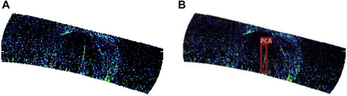
Figure 1. DMSP/SSUSI LBHL image examples. (A) Original image. (B) An example image with annotation box.

551 images with auroral arc from 2013, 2014, 2015 and 2019 collection of observations in the Northern Hemisphere form the training dataset. The test dataset consists of 1779 Images with auroral arc and 12066 without auroral arc from the 2016 collection.

2.3 Data preprocessing

Based on the characteristics of auroral arcs and the relationship between most auroral arcs and auroral oval, two different preprocessing methods are applied before training.

Preprocessing method 1: Use the original image with a size of 390 × 350 pixels. In order to meet the model’s requirements for input image size, the image is upsampled to 640 × 640 pixels to obtain Dataset1.

Preprocessing method 2: Noticed that most auroral arcs appear on the inner side of the polar boundary of the auroral oval, and the dayside auroral oval is sometimes too narrow, which is difficult to distinguish from the morphology. In order to avoid this situation, the 128 × 128 pixels portion in the middle of the original image is extracted, which not only preserves the polar cap area but also removes a portion of the auroral oval, resulting in Dataset2. Figure 2 is an example image after two preprocessing methods.

Figure 2

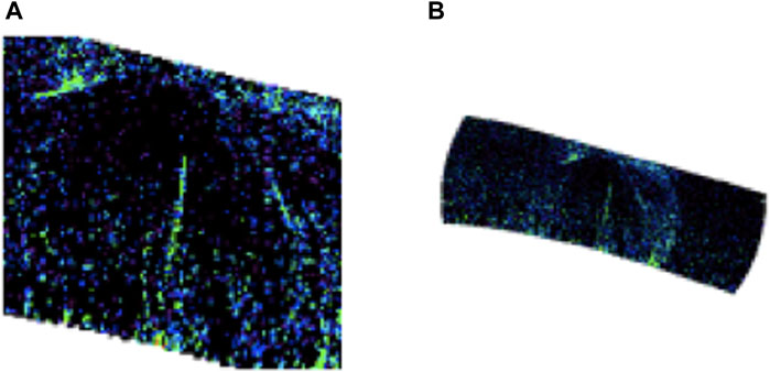
Figure 2. Sample images preprocessed by two methods. (A) Preprocessing method 1. (B) Preprocessing method 2.

In addition, random data augmentation is added during training, including image scaling, image flipping, and color gamut transformation to avoid overfitting. The image scaling operation involves scaling the image to a smaller ratio of length and width, and adding gray bars to the excess parts of the image. Image flipping operation refers to flipping the image left and right. The position of the annotation box will also change after image scaling and image flipping. Color gamut transformation refers to the process of randomly adjusting the saturation, brightness, and contrast of the original image to generate a new image.

2.4 Dataset partitioning

Considering that the current dataset of 2013, 2014, 2015, and 2019 only selected a portion of images containing auroral arcs from observations, and the dataset of 2016 is a complete dataset that had undergone manual discrimination for the presence or absence of auroral arcs. Therefore, data of 2013, 2014, 2015, and 2019 are used as the training set, and data from the entire year of 2016 as the testing set in order to comprehensively evaluate the generalization performance of the model. The training set is randomly divided into validation sets in a ratio of 4:1. The same dataset partitioning process are conducted for both Dataset1 and Dataset2. The number of images and annotation boxes on the training set, validation set, and test set are shown in Table 1. There is a sufficient number of PCAs on the training, validation, and testing sets, which can be used for model training and testing.

Table 1

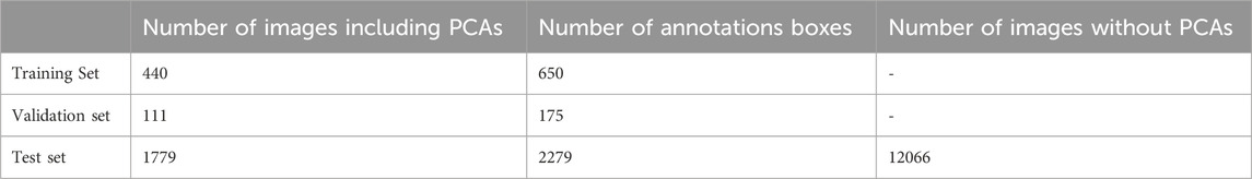
Table 1. Number of images and annotation boxes on training, validation, and testing sets.

3 Experimental methods

The previous section introduced the data preprocessing process and dataset partitioning. The experimental methods will be introduced in this section. The overall experimental process is shown in Figure 3. During the training process, the Training set1 and the Training set2 which are corresponding to the Dataset1 and the Dataset2 respectively were used to train the neural network (the YOLOX embedded with CBAM) to obtain two detectors, the Detector1 and the Detector2. Then, input the corresponding Test set1 and the Test set2 to obtain the Results1 and the Results2 for two detection boxes respectively during the testing process. Finally, the two are integrated through the intersection algorithm to obtain the final detection result. The neural network structures will be introduced in the following section, including the YOLOX and the YOLOX embedded with CBAM, as well as the intersection ensemble algorithms.

Figure 3

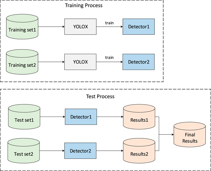
Figure 3. Schematic diagram of the training and testing processes.

3.1 YOLOX

The YOLOX is a neural network structure proposed by Kuangsi for object detection, which has significant improvements on various public datasets compared to the previous generation of the YOLOv5. Figure 4 is a schematic diagram of the overall structure of the YOLOX, consisting of three parts: the backbone feature extraction network CSPDarknet, the Feature Pyramid Network (FPN) and Path Aggregation Network (PAN), and the decoupling head YOLOHead. The backbone feature extraction network will extract features from the input images and output feature maps of different sizes. The feature pyramid network and path aggregation network will further fuse these feature maps to obtain enhanced features. Finally, the decoupling head is used to determine the target category, prediction box position, and whether the target is included.

Figure 4

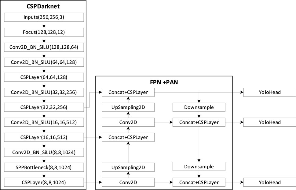
Figure 4. Schematic diagram of YOLOX model structure.

3.2 YOLOX embedded with CBAM

CBAM (Convolutional Block Attention Module) is a lightweight attention module. For an intermediate feature map, CBAM infers the attention map along the channel and spatial dimensions, and then multiplies the attention map with the input feature map for adaptive feature modification. After experimental verification, adding CBAM modules to various classic neural network structures can better focus on recognizing target objects. Therefore, this article embeds CBAM modules into the YOLOX network, and the YOLOX structure after embedding CBAM is shown in Figure 5. We have added three CBAM modules between the backbone feature extraction network and the feature pyramid network to perform an attention enhancement on the features extracted by the backbone feature extraction network.

Figure 5

Figure 5. Schematic diagram of YOLOX embedded with CBAM model structure.

3.3 Loss functions

For YOLOX and YOLOX embedded with CBAM, the loss function during the training process are shown in Equation 1. The loss function consists of three parts: bounding box regression loss, target object loss, and classification loss. In the Equation, N is the number of output layers, B is the number of targets in the grid, SxS is the number of grids divided, ${\lambda }_1$、 ${\lambda }_2$ and ${\lambda }_3$ are the weights of the three types of losses. The bounding box regression loss is achieved by calculating the CIoU of the real box and the predicted box, as shown in Equations 2–4, where $b_p$ and $b_{gt}$ are the predicted box and the annotated box respectively, $w_{gt}$ and $h_{gt}$ are the width and height of the annotated box, $w_p$ and $h_p$ are the width and height of the predicted box, $\rho$ represents the distance between the center points of the two boxes, c is the farthest distance between the boundaries of the two boxes, $\alpha$ is the weight coefficient of v. Target object loss is the calculation of whether a feature point contains an object. The feature points corresponding to the true box are considered positive samples, while the rest are considered negative samples. Therefore, the cross entropy loss is calculated based on the positive and negative samples and the predicted results of whether the feature point contains an object. The classification loss is the cross entropy loss that calculates the real box category and the predicted box category. Target object loss and classification loss can be expressed by Equation 5, where n is the number of samples, y is the predicted result, x is the true label, and is the sigmoid function.

${Loss}_{total}={\displaystyle \sum _i^N}\left({\lambda }_1{Loss}_{reg}+{\lambda }_2{Loss}_{obj}+{\lambda }_3{Loss}_{cls}\right)={\displaystyle \sum _i^N}\left({\lambda }_1{\displaystyle \sum _j^{B_i}}{L}_{{CIoU}_j}+{\lambda }_2{\displaystyle \sum _j^{S_i\times S_i}}{L}_{{BCE}_j}+{\lambda }_3{\displaystyle \sum _j^{B_i}}{L}_{{BCE}_j}\right)(1)$

$L_{CIoU}=1-IoU+\frac{{\rho }^2\left(b_p,b_{gt}\right)}{c^2}+\alpha v(2)$

$IoU=\frac{\left|b_p\cap b_{gt}\right|}{\left|b_p\cup b_{gt}\right|}(3)$

$v=\frac{4}{{\pi }^2}{\left(\mathit{arctan}\frac{w_{gt}}{h_{gt}}-\mathit{arctan}\frac{w_p}{h_p}\right)}^2(4)$

$L_{BCE}=\frac{1}{n}{\displaystyle \sum _i^n}\left[y_i\log \left(\sigma \left(x_i\right)\right)+\left(1-y_i\right)\log \left(1-\sigma \left(x_i\right)\right)\right](5)$

3.4 Transfer learning

Due to the limited number of auroral arc images, the learning ability of neural networks for auroral arc features is limited. The complex network structure is prone to overfitting on small sample datasets. Therefore, the transfer learning is utilized here. Transfer learning refers to applying knowledge learned from other tasks to new tasks, where the learned knowledge is called the source domain and the knowledge to be learned is called the target domain. The COCO dataset (https://cocodataset.org) is a large-scale dataset commonly used for object detection, consisting of over 330000 images, 1.5 million targets, and a total of 80 target categories. It is a commonly used source domain dataset in transfer learning. The auroral arc dataset is the target domain. The data distribution of the two is significantly different, and the learning tasks are different, so a model-based transfer learning method is used. Firstly, the network is pretrained on the source domain dataset, using the YOLOX-s pretraining weights provided by Kuangshi (https://github.com/STATWORX/ptu-stamping-insights-yolox/). Then, the weights of the backbone network are retained as the initial values for training on the target domain dataset. Subsequently, the parameters of the backbone network are tuned during training until the loss function converges, resulting in the final network weights.

3.5 Experimental parameter settings

During training, the Stochastic Gradient Descent with Momentum (SGDM) method is used for parameter updates, with an initial learning rate of 1e-2. The learning rate is updated using the Cosine Annealing algorithm (Loshchilov and Hutter, 2017), with a batch size of 8 for each iteration and an initial iteration of 200 epochs.

3.6 Intersection integration algorithm

After completing the training of the two models, auroral arc detection will be performed on the images of the test set separately. The two results will be mapped onto the original images and integrated using the intersection ensemble algorithm. The pseudocode for the intersection integration algorithm is shown in Figure 6. For an image, if both Results1 and Results2 have prediction boxes, and the intersection to union ratio of their prediction boxes is higher than the preset ratio threshold, it is judged that the image has an aurora arc. Both prediction boxes are retained as references. On the contrary, it is judged that there is no auroral arc in the graph.

Figure 6

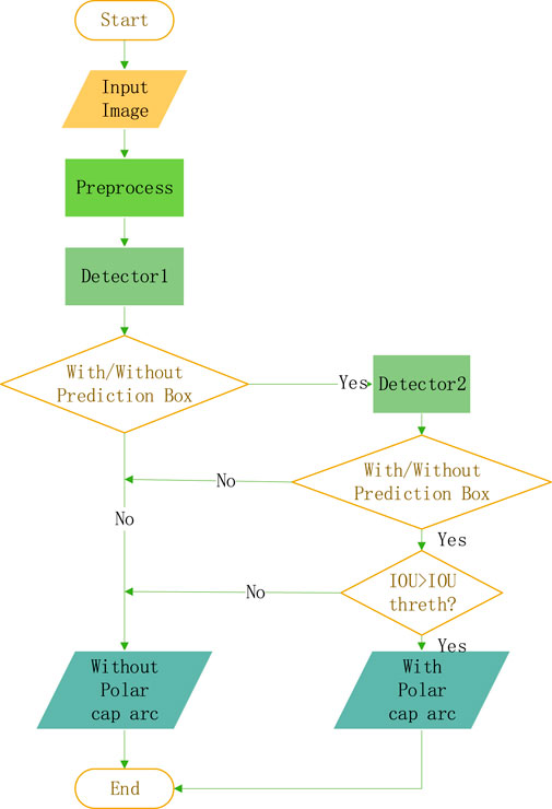
Figure 6. And-Ensembling algorithm flowchart.

4 Results and analysis

According to the experimental scheme in the previous section, we use the data sets obtained by the two preprocessing methods to train YOLOX and YOLOX embedded in CBAM respectively. We detect them on the test set, and then integrate them through the intersection integration algorithm. This section will first show the training process of the model, then evaluate the model from the two aspects of Aurora arc event recognition and Aurora arc position detection, and finally analyze the results.

4.1 Model training

The training process of detector1 and detector2 is shown in Figure 7. The left figure is the loss curve trained with dataset1, and the right figure is the loss curve trained with dataset2. The validation loss of the two models began to converge at about 150 epochs, while the training loss was still declining. Therefore, the training was stopped before 200 epochs, and the parameters on the epochs with the lowest loss in the validation set were selected as the final model parameters.

Figure 7

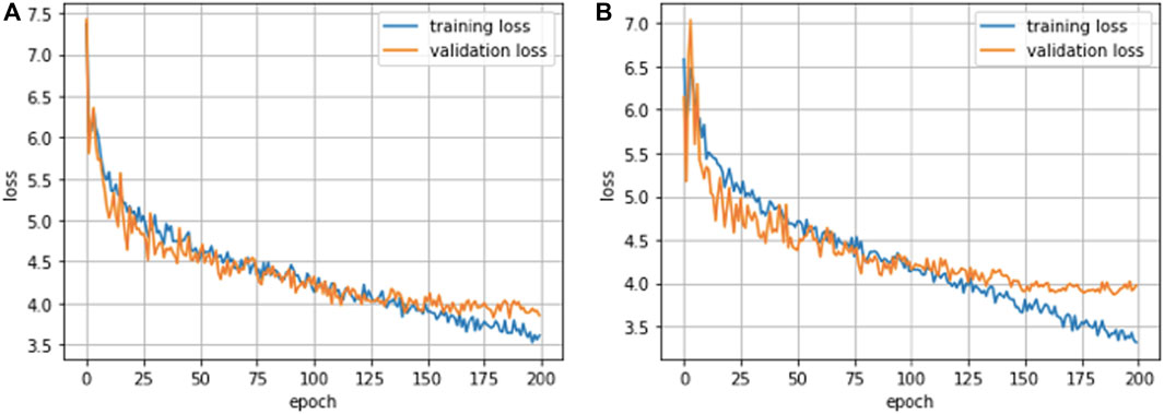
Figure 7. (A): the training process of detector 1; (B): the training process of detector2.

4.2 Evaluation index

4.2.1 Evaluation index of auroral arc event recognition

Evaluation of auroral arc event recognition refers to the accuracy of the evaluation model in judging whether the image contains auroral arcs, that is, the evaluation of a binary classification problem. Since Aurora arc is an event with small probability, precision, recall and F1 will be used as indicators for classification evaluation.

According to the combination of real category labels and prediction categories, all test samples can be divided into four cases: true positive, false positive, true negative, and false negative. The TP, FP, TN, and FN will show the corresponding sample numbers respectively. The confusion matrix of PCA classification results is shown in Table 2.

Table 2

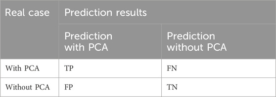
Table 2. PCA classification confusion matrix.

Further define the following parameters. The precision, recall and F1 are defined in the Equations 6–8:a) Precision refers to the proportion of correct predictions in all images predicted to contain auroral arcs, reflecting the accuracy of “no misjudgment” of the model.

$Precision=\frac{TP}{TP+FP}(6)$

b) Recall refers to the proportion of all images predicted to contain auroral arcs that are correctly predicted, reflecting the sensitivity of the model to “not miss judgment”.

$Recall=\frac{TP}{TP+FN}(7)$

c) F1 is the harmonic average based on precision and recall.

$\frac{1}{F1}=\frac{1}{2}\cdot \left(\frac{1}{Precision}+\frac{1}{Recall}\right)(8)$

4.2.2 Evaluation index of auroral arc position detection

Auroral arc position detection and evaluation refers to the accuracy of the evaluation model for auroral arc position detection, in which the intersection union ratio IOU is used to measure the overlap of the prediction box and the annotation box.

According to the relationship with the annotated box, a prediction box can be divided into one of the following four categories. The TP, FP, FN and TN are defined in the Equations 9–12 based on the confidence and IOU:

$\text{TP}:\left\{Conf>P_{thresh}\text{\hspace{0.17em}and\hspace{0.17em}}IOU>{IOU}_{thresh}\right\}(9)$

$\text{FP}:\left\{Conf>P_{thresh}\text{\hspace{0.17em}and\hspace{0.17em}}IOU<{IOU}_{thresh}\right\}(10)$

$\text{FN}:\left\{Conf<P_{thresh}\text{\hspace{0.17em}and\hspace{0.17em}}IOU>{IOU}_{thresh}\right\}(11)$

$\text{TN}:\left\{Conf<P_{thresh}\text{\hspace{0.17em}and\hspace{0.17em}}IOU<{IOU}_{thresh}\right\}(12)$

above, $P_{thresh}$ and ${IOU}_{thresh}$ are constant from 0 to 1, which are determined by task requirements.

Further define the following parameters in Equations 13–15:

a) Precision refers to the proportion of correct predictions in all prediction boxes, reflecting the accuracy of the model “not misjudging the background as the target”.

$Precision=\frac{TP}{TP+FP}=\frac{TP}{\text{All}\text{prediction}\text{boxes}}(13)$

b) Recall refers to the proportion correctly predicted in all annotation boxes, reflecting the sensitivity of the model to “not misjudge the target as the background”.

$Recall=\frac{TP}{TP+FN}=\frac{TP}{\text{All}\text{annotation}\text{boxes}}(14)$

c) Average precision (AP): change the confidence threshold from 0 to 1, calculate each corresponding precision and recall, and draw a PR performance curve of a certain category. The enclosed area is AP.

$\text{AP}={\int }_0^1{P}_{thresh}\left(r\right)dr(15)$

In this paper, precision, recall and AP are used as performance indicators of auroral arc position detection.

4.3 Experimental results

4.3.1 Event identification results

During the test, all data on the test set are detected by detector1 and detector2 respectively. For detector1 and detector2, only the prediction frames with confidence greater than 0.5 are retained, and all prediction frames less than 0.5 are discarded. The images with prediction frames are judged as PCA. Then the detection results of the two methods are integrated by the And-Ensembling algorithm, in which the IOU thresholds are 0, 0.3 and 0.5 respectively. Table 3 shows the index results of detector1, detector2 and the ensemble.

Table 3

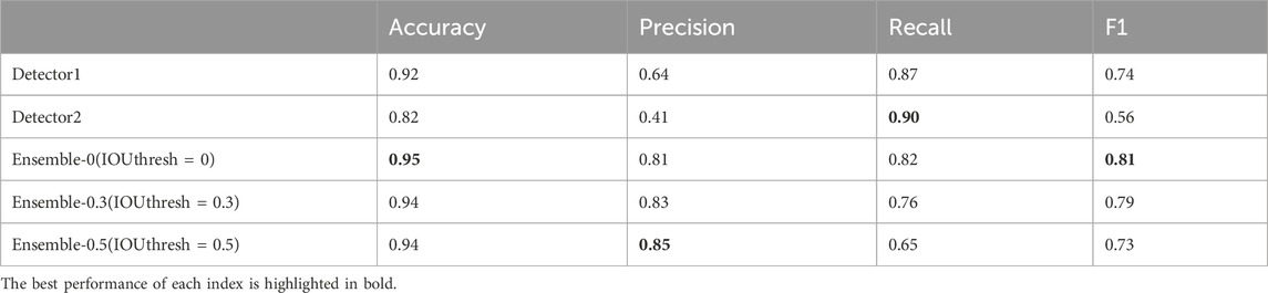
Table 3. List of index results of three methods.

It could be found that compared with the separate detector1 and detector2, the ensemble results are relatively good, especially in accuracy, precision and F1. When the IOU threshold is 0, the accuracy of ensemble is the highest, 0.95, and F1 is also the highest, 0.81. When the IOU threshold is 0.5, the precision rate of ensemble is the highest, which is 0.85. With the increase of IOU threshold, the precision rate of assembled increases. This is because a part of the prediction frames that are not the same detection target can be eliminated through the IOU threshold, so reduce the misjudgment. The maximum recall rate obtained by detector2 is 0.90, while the recall rate of the ensemble will decrease sharply with the increase of IOU threshold. Similarly, the omission of judgment will be greatly increased due to the elimination of many prediction frames. When the IOU threshold is 0, that is, when the prediction box is not eliminated through the IOU, the recall rate is the highest among the ensemble, which is only 8% lower than that of detector2 with the highest recall rate, but the precision rate is 40% higher than that of detector2, 17% higher than that of detector1, and F1 is also 7% and 25% higher than that of the other two detectors, respectively. It is proved that the accuracy of the results after the integration of two detectors is better than that of the independent results of each detector.

It could be found from Table 3 that the selection of IOU threshold has a significant impact on the results. Therefore, the IOU threshold is changed from 0 to 0.95 in steps of 0.05, and the scores of four indices corresponding to each threshold are calculated, thus Figure 8 is obtained. The accuracy, precision, and F1 all decrease with the increase of IOU threshold, with a relatively small decrease in accuracy, always higher than 0.8. This is mainly because the dataset contains a large number of images without PCA, and the model can more accurately judge these images, thereby greatly improving accuracy. The recall rate and F1 remain around 0.8 when the IOU threshold is less than 0.3, with a slight decrease before 0.5, but still around 0.7 and a sharp decrease between 0.5 and 0.95, indicating that the IOU threshold has a significant impact on recall rate and F1. The precision will increase with the increase of IOU threshold, from 0.81 to a maximum of 0.94. There is a significant negative correlation between precision and recall, and the decrease in recall also affects F1, indicating that using the IOU threshold to remove prediction boxes that may not have the same target will improve precision by sacrificing recall. Taking into account several evaluation indices, we will discuss the IOU thresholds of 0, 0.3, and 0.5, respectively.

Figure 8

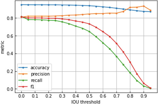
Figure 8. The variation curve of various evaluation index with IOU threshold.

In addition to the impact of IOU threshold on the detection results, the confidence threshold also affects the detection results. For an aurora image dataset of unknown category, relevant researchers prefer that the images containing PCA detected by the detection model are relatively accurate, so the precision rate is more important than the recall rate. Therefore, here, the confidence threshold is changed from 0 to 0.9 in steps of 0.05, and the precision rate corresponding to each threshold is calculated, thus Figure 9 is obtained. With the increase of confidence threshold, the precision of various models also increases. The precision of ensembled algorithm is always higher than that of two detectors, which fully proves the effectiveness of And-Ensembling algorithm.

Figure 9

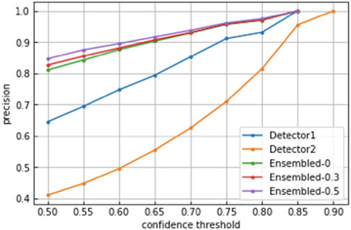
Figure 9. The variation curve of precision with confidence threshold.

Figure 10 shows twos examples where the ensemble results correct the misjudgment by detector1 and detector2, and the corresponding confidence is given above the prediction box. Figure 10A is the detection result of detector 1 on the LBHL band image observed by DMSP F16 on the orbit 63507 on 8 February 2016, Figure 10B is the detection result of detector 2 on the LHBL band image observed by DMSP F16 on the orbit 63153 on 14 January 2016. In the original images of Figures 10A, B, there was no PCA structure after manual judgment. In the experimental results, detector1 in Figure 10A misjudged the part of the auroral oval residue after cutting as PCA, while detector2 had no prediction box on the image, so the result of the two was that the image had no PCA. In Figure 10B, detector1 judged that there was no prediction box in the image, while detector2 misjudged the thinner auroral oval in the dayside as PCA. The ensemble result of the two is still no PCA, so the ensemble result is still correct. It is proved that the detector1 and the detector2 can make up for each other’s shortcomings, so the accuracy of the ensemble results can be greatly improved.

Figure 10

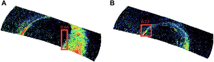
Figure 10. (A) Example image of detector2 correction misjudged by detector1. (B) Example image of detector1 correction misjudged by detector 2.

4.3.2 Position identification results

The above shows analysis of the results that whether the image contains PCA or not. In addition, the detection of PCA position is also important. Table 4 shows the evaluation results of PCA position detection.

Table 4

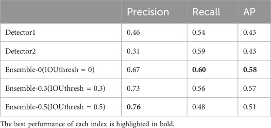
Table 4. Auroral arc position detection evaluation results.

From Table 4, it could be found that the ensemble results are better than both detector1 and detector2, especially the precision. When the IOU threshold in the And-Ensembling algorithm is gradually increased, the recall will be greatly reduced. This result is similar to the result of auroral arc event identification, which is the same as sacrificing recall to improve precision. For the task of auroral arc event identification, precision is more important than recall in order to ensure that the detected image or prediction box is more accurate and does not contain the wrong image or target as far as possible.

Figure 11 shows the correctly detected images in six different cases, which are obtained by ensemble results when the IOU threshold is 0.5 and the confidence threshold is 0.5. The green prediction box is detected by the detector1, the red prediction box is detected by the detector2, and the corresponding confidence is marked in the upper right corner of each figure. The arc in Figure 11A extends from the dawn side across the entire polar cap area to the dayside, which is a typical transpolar cap auroral arc (TPA). The arc in Figure 11B is a typical polar cap arc extending from the auroral oval near 6mlt, and the size is smaller compared with Figure 11A. The arc in Figure 11C extends from the auroral oval in the dusk side across the polar cap area and connects to the auroral oval in the dayside. It belongs to TPA and can also be called as the theta aurora. Figure 11D shows an isolated small-scale auroral arc located in the polar cap region. The arc only connects the auroral oval in the one side. From Figures 11A–D, it is shown that the model can detect both large-scale TPAs and small-scale isolated auroral arcs. Figure 11E contains two polar cap arcs. On the left is a large-scale TPA, and on the right is a small-scale auroral arc extending from the midnight, which shows that the model can also accurately detect the situation that a figure contains multiple PCAs. Figure 11F contains a lot of noises, but the model still detects the polar cap arc, which proves that the model has a certain anti-noise ability.

Figure 11

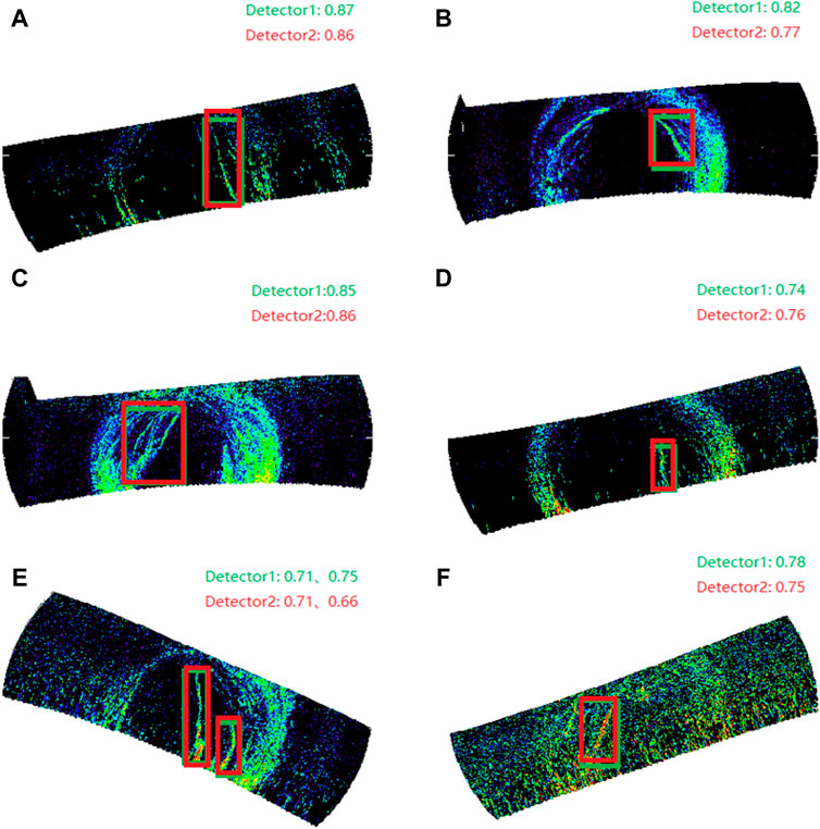
Figure 11. Six example images which are detected correctly (A) Typical dawn side TPA (B) Dawn side polar cap arc (C) Typical dusk side TPA (D) Isolated small size auroral arc (E) Two polar cap arcs in one figure (F) Detection with noises.

5 Conclusions

Aiming at the problem of auroral arc identification in satellite observation images, this paper first proposes an image preprocessing method based on the characteristics of the polar cap arc, and divides the dataset according to the time characteristics of the data. Two kinds of preprocessed datasets are used to train the YOLOX target detection model respectively, and a detection result integration method is proposed. The results show that the integrated results are better than those before And-Ensemble, especially the precision rate. The influence of threshold parameters on the detection results is discussed. According to the real detection effect, the reasons for improving the effect are analyzed, and an accurate detection example is given, which proves that the current model and integration method can effectively detect the auroral arc in a variety of situations.

The polar cap arcs (PCA) are generally rare events, they are found in auroral images during only 10%–16% of the time (Kullen et al., 2002; Fear and Milan, 2012a). The percentage is also close to our cases in the test set of 2016 collections. In this task, the background auroral oval is the noise. In auroral science, the auroral oval is formed by the energetic particles from the closed field line while the polar cap arcs are due to the open field line particles. However, there are many different features of the polar cap arcs. For example, the Theta aurora/transpolar arc, monopolar cap arc, multiple polar cap arc, space hurricanes etc as mentioned above. They are believed to have different physics mechanisms. To discovery the mechanism of the formation and evolution of different forms of polar cap arc, statistical study should be conducted. Find more cases is the key point of the statistical study. In this situation, it motivates us to apply the deep learning tools to classify the polar cap arcs, and finally find the physics features for different types of arcs.

Data availability statement

The original contributions presented in the study are included in the article/supplementary material, further inquiries can be directed to the corresponding author.

Author contributions

YL: Writing–original draft, Writing–review and editing, Conceptualization, Data curation, Formal Analysis, Investigation, Methodology, Software, Supervision, Validation, Visualization. JJ: Conceptualization, Data curation, Investigation, Methodology, Software, Validation, Visualization, Writing–original draft. JZ: Data curation, Formal Analysis, Investigation, Software, Validation, Writing–review and editing. YW: Conceptualization, Data curation, Formal Analysis, Resources, Writing–review and editing. XW: Conceptualization, Data curation, Formal Analysis, Resources, Writing–review and editing. ZZ: Funding acquisition, Project administration, Resources, Writing–review and editing.

Funding

The author(s) declare that financial support was received for the research, authorship, and/or publication of this article. This work was supported by the National Key Research and Development Program of China, Grant No. 2022YFF0711400. This work was also supported by the 14th Five-year Network Security and Informatization Plan of Chinese Academy of Sciences, Grant No. CAS-WX2022SDC-XK15; and the Informatization Plan of Chinese Academy of Sciences, Grant No. CAS-WX2022SF-0103. Shandong Provincial Natural Science Foundation (Grant ZR2022MD034, ZR2022QD077), Xiaomi Young Talents Program, and the foundation of the National Key Laboratory of Electromagnetic Environment (Grant 6142403180204).

Acknowledgments

We acknowledge the National Space Science Data Center of China (https://www.nssdc.ac.cn) for providing data resources/computing services/data analysis environment. The Space Science Data Fusion Computing Platform of the National Space Science Center provided computing services.

Conflict of interest

The authors declare that the research was conducted in the absence of any commercial or financial relationships that could be construed as a potential conflict of interest.

Publisher’s note

All claims expressed in this article are solely those of the authors and do not necessarily represent those of their affiliated organizations, or those of the publisher, the editors and the reviewers. Any product that may be evaluated in this article, or claim that may be made by its manufacturer, is not guaranteed or endorsed by the publisher.

References

Elphinstone, R. D., Jankowska, K., Murphree, J. S., and Cogger, L. L. (1990). The configuration of the auroral distribution for interplanetary magnetic field B_z northward, 1, IMF B_x and b_y dependencies as observed by the Viking satellite. J. Geophys. Res. 95, 5791–5804. doi:10.1029/ja095ia05p05791

CrossRef Full Text | Google Scholar

Fear, R. C., and Milan, S. E. (2012a). The IMF dependence of the local time of transpolar arcs: implications for formation mechanism. J. Geophys. Res. 117, A03213. doi:10.1029/2011JA017209

CrossRef Full Text | Google Scholar

Frank, L. A., Craven, J. D., Gurnett, D. A., Shawhan, S. D., Burch, J. L., Winningham, J. D., et al. (1986). The theta aurora. J. Geophys. Res. 91, 3177–3224. doi:10.1029/JA091iA03p03177

CrossRef Full Text | Google Scholar

Ge, Z., Liu, S., Wang, F., Li, Z., and Sun, J. (2021). YOLOX: exceeding YOLO series in 2021. ArXiv, abs/2107.08430.

Google Scholar

Girshick, R. (2015). “Fast r-cnn[C],” in Proceedings of the IEEE international conference on computer vision, 1440–1448.

Google Scholar

Girshick, R., Donahue, J., Darrell, T., and Malik, J. (2014). “Rich feature hierarchies for accurate object detection and semantic segmentation,” in Proceedings of the IEEE conference on computer vision and pattern recognition (CVPR), 580–587.

CrossRef Full Text | Google Scholar

Gussenhoven, M. S. (1982). Extremely high latitude auroras. J. Geophys. Res. 87, 2401–2412. doi:10.1029/JA087iA04p02401

CrossRef Full Text | Google Scholar

Hardy, D. A., Schmitt, L. K., Gussenhoven, M. S., Marshall, F. J., Yeh, H. C., Shumaker, T. L., et al. (1984). Precipitating electron and ion detectors (SSJ/4) for the Block 5D/flights 6 – 10 DMSP satellites: calibration and data presentationRep., air force geophys. Lab., hanscom air force base.

Google Scholar

Hosokawa, K., Kullen, A., Milan, S., Reidy, J., Zou, Y., Frey, H., et al. (2020). Aurora in the polar cap: a review. SPACE Sci. Rev. 216 (1), 15. doi:10.1007/s11214-020-0637-3

CrossRef Full Text | Google Scholar

Hu, J., Shen, L., and Sun, G. (2018). “Squeeze-and-excitation networks[C],” in Proceedings of the IEEE conference on computer vision and pattern recognition, 7132–7141.

Google Scholar

Krizhevsky, A., Sutskever, I., and Hinton, G. E. (2017). Imagenet classification with deep convolutional neural networks. Commun. ACM 60 (6), 84–90. doi:10.1145/3065386

CrossRef Full Text | Google Scholar

Kullen, A., Brittnacher, M., Cumnock, J. A., and Blomberg, L. G. (2002). Solar wind dependence of the occurrence and motion of polar auroral arcs: a statistical study. J. Geophys. Res. 107, 1362. doi:10.1029/2002JA009245

CrossRef Full Text | Google Scholar

Lassen, K., and Danielsen, C. (1978). Quiet-time pattern of auroral arcs for different directions of the interplanetary magnetic field in the Y-Z plane. J. Geophys. Res. 83, 5277–5284. doi:10.1029/ja083ia11p05277

CrossRef Full Text | Google Scholar

Liu, Y., Shao, Z., and Hoffmann, N. (2021). Global attention mechanism: retain information to enhance channel-spatial interactions. arxiv preprint arxiv:2112.05561.

Google Scholar

Loshchilov, L., and Hutter, F. (2017). “SGDR: stochastic gradient descent with warm restarts[C],” in Iclr.

Google Scholar

Lu, S., Xing, Z.-Y., Zhang, Q.-H., Zhang, Y.-L., Ma, Y.-Z., Wang, X.-Y., et al. (2022). A statistical study of space hurricanes in the Northern Hemisphere. Front. Astron. Space Sci. 9, 1047982. doi:10.3389/fspas.2022.1047982

CrossRef Full Text | Google Scholar

Meng, C.-I. (1981a). Polar cap arcs and the plasma sheet. GeophlJs. Res. Lett. 8, 273–276. doi:10.1029/gl008i003p00273

CrossRef Full Text | Google Scholar

Meng, C.-I. (1981b). The auroral electron precipitation during extremely quiet geomagnetic conditions. J. Geophys. Res. 86, 4607–4627. doi:10.1029/ja086ia06p04607

CrossRef Full Text | Google Scholar

Moen, J., Sandholt, P. E., Lockwood, M., Egeland, A., and Fukui, K. (1994). Multiple, discrete arcs on sunward convecting field lines in the 1415 MLT region. J. Geophys. Res. 99, 6113–6123. doi:10.1029/93ja03344

CrossRef Full Text | Google Scholar

Murhree, J. S., and Cogger, L. L. (1981). Observed connections between apparent polar cap features and the instantaneous diffuse auroral oval. Planet. Space Sci. 29, 1143–1149. doi:10.1016/0032-0633(81)90120-3

CrossRef Full Text | Google Scholar

Paxton, L. J., Morrison, D., Zhang, Y., Kil, H., Wolven, B., Ogorzalek, B. S., et al. (2002). “Validation of remote sensing products produced by the special sensor ultraviolet scanning imager (SSUSI): a far UVimaging spectrograph on DMSP F-16,” in Proceedings of SPIE—the international society for optical engineering, 4485.

CrossRef Full Text | Google Scholar

Redmon, J., Divvala, S., Girshick, R., and Farhadi, A. (2016). “You only look once: unified, real-time object detection,” in Proceedings of the CVPR.

CrossRef Full Text | Google Scholar

Ren, S., He, K., Girshick, R. B., and Sun, J. (2015). Faster R-CNN: towards real-time object detection with region proposal networks. IEEE Trans. Pattern. Anal. Mach. Intell. 39, 1137–1149. doi:10.1109/TPAMI.2016.2577031

PubMed Abstract | CrossRef Full Text | Google Scholar

Troshichev, O. A. (1990). Global dynamics of the magnetosphere for northward IMF conditions. J. Atmos. Terr. Phys. 52 (12), 1135–1154. doi:10.1016/0021-9169(90)90083-Y

CrossRef Full Text | Google Scholar

Wang, Q., Wu, B., Zhu, P. F., Li, P., Zuo, W., and Hu, Q. (2019). “ECA-Net: Efficient channel attention for deep convolutional neural networks,” in 2020 IEEE/CVF Conference on Computer Vision and Pattern Recognition (CVPR), 11531–11539.

Google Scholar

Wang, X. Y., Zhang, Q. H., Wang, C., Zhang, Y. L., Tang, B. B., Xing, Z. Y., et al. (2023). Unusual shrinkage and reshaping of Earth’s magnetosphere under a strong northward interplanetary magnetic field. Commun. Earth Environ. 4 (1), 31. doi:10.1038/s43247-023-00700-0

CrossRef Full Text | Google Scholar

Woo, S., Park, J., Lee, J. Y., and Kweon, I. S. (2018). Cbam: convolutional block attention module. Cham: Springer. doi:10.1007/978-3-030-01234-2_1

CrossRef Full Text | Google Scholar

Zanyang, X., Zhang, Q., Han, D., Zhang, Y., Sato, N., Zhang, S., et al. (2018). Conjugate observations of the evolution of polar cap arcs in both hemispheres. J. Geophys. Res. Space Phys. 123, 1794–1805. doi:10.1002/2017JA024272

CrossRef Full Text | Google Scholar

Zhang, Q.-He, Zhang, Y.-L., Wang, C., Lockwood, M., Yang, H.-G., Tang, B.-B., et al. (2020). Multiple transpolar auroral arcs reveal insight about coupling processes in the Earth’s magnetotail. Proc. Natl. Acad. Sci. U. S. A. (PNAS) 117 (28), 16193–16198. doi:10.1073/pnas.2000614117

PubMed Abstract | CrossRef Full Text | Google Scholar

Zhang, Q.-He, Zhang, Y.-L., Wang, C., Oksavik, K., Lyons, L. R., Lockwood, M., et al. (2021). A space hurricane over the Earth’s polar ionosphere. Nat. Commun. 12, 1207. doi:10.1038/s41467-021-21459-y

PubMed Abstract | CrossRef Full Text | Google Scholar

Zhu, L., Sojka, J. J., Schunk, R. W., and Crain, D. J. (1994a). Model study of multiple polar cap arcs: occurrence and Spacing. Geophys. Res. Lett. 21, 649–652. doi:10.1029/94gl00562

CrossRef Full Text | Google Scholar

Zhu, L., Sojka, J. J., Schunk, R. W., and Crain, D. J. (1994b). Theoretical study of polar cap arcs: time-dependent model and its applications. Radio Sri. 29, 283–292. doi:10.1029/93rs01508

CrossRef Full Text | Google Scholar