Inter-calibration of Infrared Channels of Geostationary Meteorological Satellite Imagers

This article examines a method of inter-calibration for MSU-GS imager of the Russian Geostationary Earth Orbit (GEO) satellite Elektro-L No. 2. Since the launch (December 11, 2015), the satellite's radiation cooler has been operating in an abnormal mode, so the calibration of the IR channels of the MSU-GS imager differed from that pre-flight and, in general, could have a daily variability. To ensure the satellite's further operation in orbit, it was necessary to calibrate imager channels at a frequency that would allow to identify daily calibration course to detect and compensate its sources. In order to do this, we have developed a special method of GEO-GEO inter-calibration. The calibration of MSU-GS was performed using SEVIRI imager installed on the GEO satellite Meteosat-10. SEVIRI was chosen as a reference instrument because its spectral channels are similar to those of MSU-GS. The MSU-GS was calibrated according to the regressions calculated from the simultaneous images of the field of regard selected between the sub-satellite points. The dynamic brightness temperature range was determined by deep convective clouds in high troposphere and warm ocean surface. Using the proposed method of inter-calibration, it was possible to confirm the absence of a significant daily variation of the calibration since November 2017. The amplitude of the variation smoothly increases from ~0.2 K at high (~300 K) BTs to ~1.0 K when the brightness temperature decreased to 200 K. These estimates allow the use of the Fourier spectrometer IKFS-2 installed on the Russian Low-Earth-Orbit (LEO) satellite Meteor-M No. 2 to verify the developed GEO-GEO scheme of inter-calibration. Despite the specifics of the situation on board Elektro-L No. 2, the proposed method of GEO-GEO inter-calibration can be applied to radiometers of other neighboring satellites that differ in SSP and spatial resolution.

Introduction

Remote sensing data from Geostationary Earth Orbit (GEO) satellites are widely used for continuous monitoring of the atmosphere, ocean and the land. The high quality of information is ensured by pre-flight calibration and on-board calibration during the flight tests of the radiometer. However, occasionally the radiometric characteristics of the on-board imagers can change due to the degradation of the photosensitive elements or the instability of their operating conditions. Often, these changes cannot be envisaged before the launch of the satellite or offset by on-board calibration. Therefore, there is a need for inter-calibration of satellite instruments directly in the orbit, when measurements from one device are verified by measurements from a reference instrument, which is installed on another satellite, with more accurate and stable radiometric characteristics.

The Global Space Inter-Calibration System (GSICS) created under the aegis of the World Meteorological Organization (Goldberg et al., 2011), develops recommendations on algorithms for inter-calibration and selection of reference satellite instruments. Most often within the GSICS, GEO-LEO inter-calibration is carried out (Chander et al., 2013) when a calibrated instrument is onboard a GEO satellite. In this case, the reference instruments is installed on a Low-Earth-Orbit (LEO) satellite. The results of inter-calibration for imager MSU-GS, installed on the first satellite of the series Elektro-L, using GEO- LEO scheme are presented in Kiseleva et al. (2016). The data of IR channels of the MSU-GS imager were compared with the data of the Atmospheric Infra-Red Sounder (AIRS, Gunshor et al., 2009) that is one of the GSICS reference instruments installed onboard the LEO satellite EOS/Aqua. Verification of the used method was performed on the example of inter-calibration of imager SEVIRI/Meteosat-10 using data of spectrometer AIRS. SEVIRI is installed on the European geostationary satellite Meteosat-10 (with the Sub-Satellite Points (SSP) at the Greenwich meridian over the Atlantic Ocean), and its spectral channels are similar to those of MSU-GS.

The Russian GEO hydrometeorological satellite Elektro-L No. 2 (Asmus et al., 2012) was launched into orbit on December 11, 2015. The satellite is positioned above the equator at 76°E longitude. The radiation cooler of Elektro-L No. 2 satellite has been operating in an abnormal regime since the very beginning of it mission, which caused the temperature of the light sensor array (LSA) of the MSU-GS imager to exceed its projected value by over 10K. Because of this, the amplitude functions (AF) of the imager channels, i.e., the dependences of optical signal power at the input of the LSA on measured brightness temperature (BT) at the output, were not only different from those obtained during the preflight calibration on Earth, but also unstable in time.

When carrying out flight tests of Elektro-L No. 2 to determine the daily and inter-day variance of AF in different ranges of the measured BT and to reveal the causes of this variance, it was necessary to ensure frequent inter-calibration of the MSU-GS channels. The use of the methodology (EUMETSAT, 2016; Kiseleva et al., 2016) or similar ones based on the GEO-LEO scheme allows for inter-calibration only twice daily. This frequency is not sufficient to set the parameters of the AF daily changes or to verify their stability.

In light of this, we developed the GEO-GEO inter-calibration scheme under which both the calibrated and reference instruments were located on-board geostationary satellites. SEVIRI/Meteosat-10 imager was chosen as a reference instrument. The numbers of the MSU-GS and SEVIRI channels, their central wavelengths, and spectral ranges of the channels are similar (Andreev et al., 2015; Kiseleva et al., 2016). This SEVIRI/Meteosat-10 had been previously used in Kiseleva et al. (2016) to test the inter-calibration of the IR channels of the older imager onboard Elektro-L No. 1 satellite. In addition, SEVIRI successfully operates on other Meteosat satellites and boasts highly stable radiometric characteristics (EUMETSAT, 2007; König, 2007; Gunshor et al., 2009).

Inter-calibration was performed for the simultaneous measurement sessions of both imagers. Since the MSU-GS/Elektro-L No. 2 conduct their measurements at half-hour intervals (twice less often than SEVIRI), the maximum number of inter-calibrations per day reached 48. The spatial resolution of SEVIRI is 3 km and the MSU-GS is 4 km (https://www.wmo-sat.info/oscar/instruments/). After the image of the Earth disc is acquired, the brightness measured from the satellite's GEO for a certain viewing angle is interpolated in some way to a node of a fixed latitude-longitude grid on the Earth's surface with a non-uniform pitch centered on the sub-satellite point. Coordinates of the grid nodes are calculated in advance, based on the nadir size of the imager pixel. The number of nodes of the grid is 2784 × 2784 for MSU-GS and 3712 × 3712 for SEVIRI. Each grid node defines a cell, which we will call also a pixel because their sizes are approximately the same. When performing inter-calibration and image collocation, it is advisable to use the MSU-GS grid that has less spatial resolution.

The development of inter-calibration methodology was carried out by comparing the measurement data in the 9th channel of both instruments located in the IR atmospheric window of 10–12 μm. Due to the abnormal operation of MSU-GS, the pre-flight calibration data could be used only as approximate. Therefore, we did not take into account the effect of the differences in the Instrumental Spectral Response Function (ISRF) of the MCU-GS and SEVIRI channels on the difference in the measured BT. All bands 4–10 have identical structure. So the method described in this article may be applied to any one of them. We selected channel # 9 as the most important one for various thematic tasks. Besides, its spectral band is located in the atmospheric window so the range of measured brightness temperatures is over 100 K degrees.

A detailed description of all calibration steps is provided in the GSICS document titled Algorithm Theoretical Basis Document (ATBD; Hewison et al., 2013). This document outlines the following calibration stages: subsetting, collocation, transformation, filtering, monitoring, and correction. This sequence is used in many scientific works dedicated to inter-calibration of satellite radiometers (Hewison et al., 2013; Takahashi, 2017), mainly calibrations like GEO-LEO. There are much fewer publications discussing GEO-GEO inter-calibration (see, for example, Hillger and Schmit, 2011; Takahashi, 2017).

The coordinates of the cloud observed by the satellite are determined by the coordinates of the point of intersection of the Earth's surface by a ray starting from the satellite and passing through the cloud. During the inter-calibration (Takahashi, 2017; Yamashita, 2017) of Himawari−8 and−9, both satellites were located at the same point. Therefore, the distance between the points on the Earth's surface corresponding to the cloud for both satellites will be much shorter than the linear dimensions of the AHI pixel (2 km to nadir). Thus, the cloud will be assigned to the same pixel for both imagers regardless of its height and will not cause additional errors.

When inter-calibrating the imagers of GOES-15 and GOES-13 or imagers of GOES-15 and GOES-11 (Hillger and Schmit, 2011), the distance between the SSP by longitude was, respectively 14.5° and 45.5°. Such distance can cause the observed high cloud to be referred to different pixels of the spatial grid and, in the case of high clouds; the divergence in the measured BTs could reach 100K or more. To prevent this from happening (Hillger and Schmit, 2011), a comparison of BTs of the corresponding intensity of outgoing radiation averaged over 10 × 10 pixels (i.e., over an area of approximately 50 × 50 km²) was performed. Such averaging reduces the statistical error of comparison. However, in this case, the dynamic range of the compared BTs is significantly reduced, because radiation from cold tops of high clouds is mixed with radiation coming from warm clouds of lower layers and the underlying surface and it must increase average brightness temperature in comparison with temperature of cloudy pixels. The lack of high clouds when comparing GOES-15 and−13 may be as due to the geography and season of the comparisons so as result of averaging. For example, for the imager channel #4 (10.8 μm), there were practically no comparable BTs below 230 K.

The features of this work was that we simultaneously had to calibrate at low BTs (220 K and below), which are typical for the cloud tops at altitudes of about 15 km, and had to take into account the large (76°) distance of the Elektro-L No.2 and Meteosat-10 SSPs in longitude. Therefore, we could not use pixel-to-pixel comparison of the radiances or BTs measured MSU-GS and SEVIRI, as was done during the inter-calibration of the AHI imagers (Takahashi, 2017) installed on Himawari −8 and −9, nor by comparing the intensities averaged over large areas, as was done for imagers (Hillger and Schmit, 2011) installed on GOES. As the existing GEO-GEO inter-calibration schemes could not be used, we have developed a new method presented in this article. In general, it repeats the approach of the mentioned above ATBD (Hewison et al., 2013). At the same time, its core and the execution order is significantly different from that of other inter-calibrations discussed above. The methodology involves the following steps:

- determination of the inter-calibration field of regard (FOR) on the Earth's surface located in the middle between the SSP (along the meridian of 38°E);

- collocations of SEVIRI measurements on the latitude-longitude grid adopted for MSU-GS and the selection of uniform fragments of images obtained from two satellites;

- statistical equalization of the number of selected fragments by performing unique changes in the threshold values of the selection criterion for each instrument;

- establishment of a one-to-one correspondence between subsets of image fragments of the inter-calibration FOR from both satellites and the calculation of the average BTs for the compared pairs of fragments to obtain a regression;

- filtering out gross errors that arise when two BT fragments, which belong to different cloud formations are being compared;

- correction of geolocation errors and a new collocation of BT pairs that are being compared;

- obtaining regression relationships for inter-calibration in a wide range of BTs.

These steps will be examined in more detail below.

Methods

Inter-calibration Region

The different sub-satellite longitudes of Elektro-2 (76°E) and Meteosat-10 (0°) on the geostationary orbit mean that the region of the world observed by both satellites at a similar angle needs to be located near 38° ± 3°E. Its width is constrained within the range of ± 45° latitude. The range of the variation in Earth incidence angle corresponds to 43.9 ± 5.6°.

The land-free area of the Indian Ocean off the south-west coast of Madagascar was selected from the entire region for its high BT (290÷300 K) inter-calibration. The use of the warm ocean surface is necessary to eliminate the calibration error due to the unequal daily course of land surface temperature observed from east to west for the right-hand satellite and from west to east for the left-hand satellite. The temperature of the hillsides in the desert facing east (Elektro-2), for example, in the morning will be quite different from the temperature measured on the slopes of the same hills facing west (\Meteosat-10, 11). For the ocean surface, the BRs measured from both satellites can vary but will be the same throughout the day.

Identifying this additional region of the sea allowed us to eliminate the Sun's a.m.,/p.m. impact on the calibration constants. In case of the solid underlying surface, this impact is constituted by the diurnal difference of BTs observed from the sun-side (Elektro-2) and from the opposite-sun-side (Meteosat-10) in the morning, and the reverse situation in the evening.

The SSP and inter-calibration regions are shown in the (Figure 1).

FIGURE 1

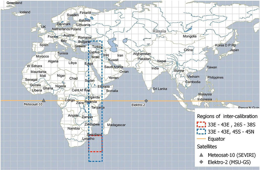
Figure 1. Inter-calibration regions MSU-GS/Elektro-2 and SEVIRI/Meteosat-10.

Selection of Uniform Images Fragments

For GEO-GEO inter-calibration processing, it is necessary to establish correspondence between fragments of the images that are obtained by both instruments. As it was noted in the Introduction, the SEVIRI image was preliminarily transformed to the MSU-GS longitude-latitude grid, i.e., converted into lower spatial resolution. The images converted to a lower spatial resolution by nearest neighbor interpolation. To make analysis more convenient, the pixels (grid points) in the inter-calibration region were selected to form a rectangular matrix with 135 columns and 1,920 rows. A similar matrix for the Madagascar region had the number of rows reduced to 200. The pixels contained in the matrix columns are located along the meridians: the difference between the maximum and minimum longitude values of the same column pixels ranges from 0 to 1.3°. Similarly, the matrix rows contain pixels, which roughly coincide with the parallels: the difference between the maximum and minimum latitude values of the same row pixels ranges from 0 to 0.1°.

Statistical reliability of the inter-calibration is ensured by simultaneous observation of the same spatially uniform fragments of the different atmospheric scenes that are observed by both satellites. In the low BT region (200–220 K) these scenes are constituted by deep convection clouds (Cb or Cu cong) with the flat top (the so-called anvil) that reaches the tropopause. In the high BT region (290–300 K) these scenes are represented by the equatorial ocean surface patches with no clouds above. The calibration in the medium BT range is carried out with using the stratus clouds of the first (stratus, St) and second (altostratus, As) levels.

The selection of uniform fragments is carried out using the standard deviation of the BT matrix (3 × 3) centered at a pixel with indices {i, j}. An image fragment can be considered uniformed if the following inequality holds:

$\begin{array}{cc}\sqrt{\frac{{\displaystyle {\sum }_{\text{k}=-1}^1{\displaystyle {\sum }_{\text{n}=-1}^1{\left({\text{T}}_{\text{i}+\text{k},\text{j}+\text{n}}-{\text{m}}_{\text{i},\text{j}}\right)}^2}}}{9-1}}<{\sigma }_{\text{h}},& (1)\end{array}$

where m_{i, j} is the mean value of the BT matrix;

σ_h is the threshold, which is selected separately for each scanner.

For MSU-GS, σ_h = 2K; for SEVIRI, σ_h = 3.4K. The choice of such values ensures there are approximately the same number (±2%) of homogeneous fragments in the inter-calibration region image of each instrument. The higher σ_h value for SEVIRI compared with σ_h for MSU-GS can offset the effect of better spatial resolution of SEVIRI (even after its conversion to the MSU-GS longitude-latitude grid), which decreases the number of fragments selected using the threshold criterion (1).

Filtration of Errors

For the response function to be corrected in the range of BTs < 275 K it is necessary to define a perfect correspondence between BTs of chosen fragments of images, mainly for fragments with clouds. As it already been mentioned, pixels of the MSU-GS image shifted to the left and pixels of the SEVIRI image shifted to the right relative to the point under the clouds are correspond with the same cloud. A distance between these pixels can reach 30–40 km for high clouds. The observation from opposite directions could lead to shading of low clouds or the underlying surface by clouds of deep convection and to difference of up to 100 K in the observed brightness temperatures. Thus, averaged on 3 × 3 area m_{i, jM} and m_{i, jS} with minimum value are picked for collocated pairs of every i-th matrix row. Index j_M points to the pixel with minimum BT value on MSU-GS image and index j_S points to the similar pixel on SEVERI image. The edge effects on border of the inter-calibration area, probable shading of low clouds by high clouds and other effects can lead to the serious errors. The verification of correspondence between j_M and j_S pixel indexes and ranges of numbers j_0M±2 and j_0S ±2 which observed fragments with BTs m_{i, jM} and m_{i, jS} must be included in realize to eliminate this errors. The middles j_0M and j_0S of allowable ranges are calculated by the projection of fragment with altitude H along the viewing ray from each satellite. The altitude H is estimated from the approximate dependence:

$\begin{array}{cc}\text{H}=\frac{\max \left({\text{T}}^{\langle \text{i}\rangle }\right)-{\text{m}}_{\text{i},{\text{j}}_{\text{S}}}}{{\text{K}}_{\text{T}}},& (2)\end{array}$

where max(T^〈i〉) - maximal BT according to SEVERI measurement in i^−th matrix row;

K_T = 6.5 K/km–troposphere average temperature coefficient (Hewitt and Jackson, 2003).

For any row there are not any MSU-GS or SEVERI image fragments obeying condition (1) or if at least one of j_M or j_S indexes is out of the allowable range, this row is not taken into account when building the regression.

Thus, we have two columns with the same length. Each column is consisted of minimal BT for row of MSU-GS or SEVIRI image. In practice, the length of column is from 300 to 400 for different meteorological conditions of the inter-calibration area.

To minimize the impact of geolocation errors, we found out the maximum of correlation coefficient R between two different columns shifting one of them on ± 3 positions. Shifted columns of minimal BT corresponding to the maximum value of R are used in procedure of building regression for the range of BTs lower than 275 K.

For the response function to be improved for the range of BT above 275 K we use the analysis of maximal values of BT for uniform (with threshold value σ_h = 0.5K) fragments of sea area located south-westerly from Madagascar. Obviously, that the maximal BTs T_max are observed when the sea area is not covered by clouds. For each satellite instruments, the average BT value is found out on the range [T_max−5, T_max]. We consider difference ${\text{T}}_{max}^{\text{MSU}}-{\text{T}}_{max}^{\text{SEV}}$ to be the calibration correction value and it is extrapolated on BT values >T_max.

Development of Calibration Relationships

The regression relationship between BT SEVIRI and MSU-GS is

$\begin{array}{cc}{\text{T}}_{\text{SEV}}\left({\text{T}}_{\text{MSU}}\right)=\text{a}+\text{b }·{\text{T}}_{\text{MSU}}+\text{c}·\text{exp}\left(-\frac{{\text{T}}_{\text{MSU}}}{{\text{K}}_{\text{T}}}\right),& (3)\end{array}$

where a, b and c are constants which were found with least squares method;

K_T = 30K – constant dimensional coefficient.

Regressions are statistically significant in the interval (Tmin, 275 K) when 7% of the values of the measured brightness temperatures are < Tmin. The level of significance of 7% is found empirically and ensures the stable behavior of the obtained curves

Now the criterion of the minimum T_min (that is obtained from high cloud measurements) choosing is when less then 7% of uniform scenes with T_MSU < T_min. As it was mentioned before,${\text{T}}_{max}^{\text{c}1}$ = 275 K. A single session is an operation cycle: any next full-disk image is produced by MSU-GS every 30 min. One image is obtained for one cycle or session over a period of 6 min. Due to such selection standard error of regression of single session is < 0.5 K. In the high-BT range the difference of T_MSU−T_SEV is defined by single BT point T_max obtained from the sea site. The rms difference is 0.1 K. The regression curve is defined in range T_min÷T_max. Extrapolation in low-BT range is not allowed. Brightness temperature of T_MSU>T_max. can be calculated using the equation

$\begin{array}{cc}{\text{T}}_{\text{SEV}}={\text{T}}_{\text{MSU}}-\left({\text{T}}_{\max }^{{}_{{}^{\text{MSU}}}}-{\text{T}}_{\max }^{{}^{\text{SEV}}}\right).& (4)\end{array}$

Consistency of calibration relationship for different parts of the dynamic range is insured by the choice of analytical dependence, which is very close to linear in the range of high (280–300 K) brightness temperatures. In addition, the calibration curve must pass through a single point Tmax obtained from the sea site. The difference between brightness temperatures more than Tmax is constant and equal to difference by Tmax. Examples of statistically significant calibration relationships obtained on April 27 (A) and on May 7 (B) at 14:30 UTC in Figure 2. The asterisk shows the position of the point for Madagascar. Black dashed lines indicate the boundaries of the 95 percent confidence interval.

FIGURE 2

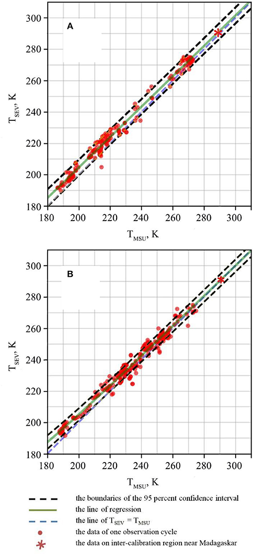
Figure 2. Examples of regressions TSEV (TMSU), 2018: (A)-April 27, 14:00 UTC; (B)-May 7, 14:30 UTC.

Results

The calibration differences ΔT = T_MSU−T_SEV were obtained through the T_SEV(T_MSU) regression relationships during simultaneous sessions of MSU-GS and SEVIRI on the fixed grid for BT more than T_min. The daily averaged ΔT as a function of the day number are shown in the Figure 3 for three BTs measured in channel #9 of MSU-GS. It is based on the statistically significant regressions obtained between May 2017 and April 2018 (the start date is 20.05.2018, which marks the beginning of MSU-GS' regular operation in orbit).

FIGURE 3

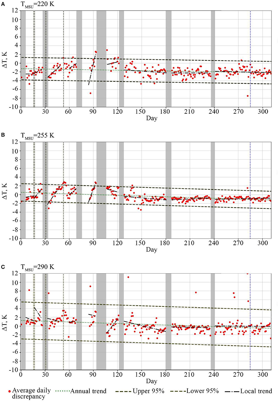
Figure 3. Annual variety of calibration differences for three BTs measured in channel #9 MSU-GS (A–220 K; B–255 K; C–290 K).

Averaged ΔT (red dots) and its trend lines (black dotted lines) have been calculated for all periods between the cleaning sessions of the of MSU-GS cooling system. The time intervals when the cooler cleaning was conducted appear as gray areas in Figure 3. Vertical yellow lines (on 16th, 17th, and 53rd days) mark the days of orbit corrections. Outliers in the plot that exceed the confidence interval are not included in the trend statistics. They are likely caused by the unstable operation of the equipment. It should be noted that there are line regressions of the calibration bias as function of day number (green lines) between the clearings of cooler radiator. Local trends were influenced by the orbit corrections too. Supposedly, the reason for this effect is a residual atmosphere density fluctuation near the cooler radiator. Calibration bias ranges in any single period of normal work were rather more than its annual variance (green dotted line). The stability of MSU-GS operation has improved (there are virtually no breaks between the regression lines) since November 2017. It is confirmed in all subsequent calibrations until May 2018. The spacecraft reversal by 180° on the vernal equinox (vertical blue line, 282nd day) performed in order to prevent the cooler from being heated by the Sun rays has no influence on this trend.

Eumetsat stopped to broadcast SEVIRI/Meteosat-10 data in February 2018, having replaced it by Meteosat-11 data (3.4°E). The inter-calibration between SEVIRI/Meteosat-11 and Russian Fourier-spectrometer IKFS-2 showed that the difference of BT as compared with SEVIRI/Meteosat-10 is < 0.1 K. As shown in Figure 3, changing the reference instrument has almost no influence on the time-sensitive stability of calibration corrections of the MSU-GS measurements.

The diurnal calibration variation of the MSU-GS channel #9 averaged for the current year (2018) is shown in Figure 4 for the same BT as in Figure 3. The systematic bias caused by the ice accumulation was taken into account using regressions of the calibration bias as a function of day number between the clearings of the cooler radiator. The analysis of the curves shows that the amplitude of the mean offset (blue curve) does not exceed 0.2 K for high BTs and gradually increases to 1 K for low temperatures. For comparison, the MSU-GS BT for 4 sessions at 05.30–07.00 UTC are shown in the figure (those marked by red triangles) were not statistically treated and obtained by processing in Siberian Centre (Novosibirsk) using preflight response function. Other values were obtained using the corrected (20.05.2018) response function in European Centre (Moscow) .The estimation of calibration diurnal amplitude for different MSU-GS BT makes it possible to use the GEO-LEO calibration scheme for developed method verification. The Fourier spectrometer IKFS-2 (Golovin et al., 2014) on board Meteor-M No.2 (Russian low-orbiting satellite) was used as the reference. During the time following Meteor-M No.2 launch in July 2014, the IKFS-2 was undergoing numerous inter-calibrations. In particular, the inter-comparison of IKFS-2 and collocated IASI and CrIS spectra shows that the discrepancies between them do not exceed measurement noise (Zavelevich et al., 2018).

FIGURE 4

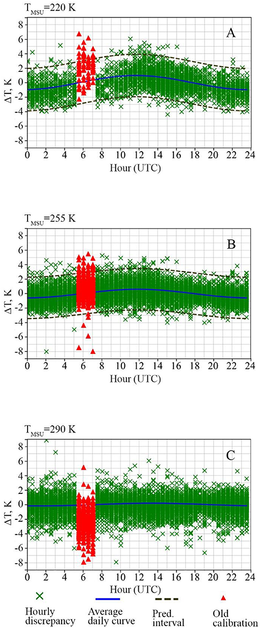
Figure 4. Averaged (during the year 2018) diurnal variation of calibration offsets in MSU-GS channel# 9 for three BTs (A–220 K; B–255 K; C–290 K).

In the range of high temperatures (290÷300 K), the diurnal variance does not exceed 0.2 K, while gradually increasing to 1 K at 200 K.

The result of the comparison of SEVIRI band 9 BT estimations is shown in Figure 5. These estimations are actually obtained by two inter-calibration schemes: GEO-GEO (by MSU-GS measurements) and GEO-LEO (by IKFS-2 measurements).

FIGURE 5

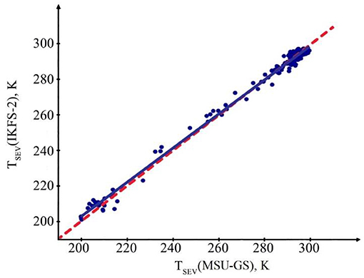
Figure 5. Comparison of SEVERI BT estimates from GEO-GEO and GEO-LEO inter-calibrations, accordingly T_SEV(MSU-GS) and T_SEV(IKFS-2). In SSP region of Elektro 2, MSU-GS BT were recalculated to T_SEV(MSU-GS) by using obtained calibration relationship. In the same region, to obtain estimates T_SEV(IKFS-2), the radiance spectra measured by IKFS-2 were convolved with SRF of SEVIRI ch.9 for MSU-GS pixels collocated with central pixels of IKFS-2.

The collocated data were picked out during March-April 2018 for Electro-L No. 2 nadir region (76°E) limited by area ±5° on longitude and latitude. For GEO-GEO scheme, MSU-GS BT were recalculated to SEVIRI measurements by using obtained calibration relationships. For comparison, we used MSU-GS pixels located in central IKFS-2 pixels, where the zenith angle deviation from nadir does not exceed 7°. In addition, for the uniform atmosphere scenes (cloud cover or lack of clouds) to be picked out, MSU-GS BT standard deviation of pixels located in IKFS-2 field of view shouldn't exceed 3 K. For the GEO-LEO scheme, the radiance spectrum measured by IKFS-2 was convolved with the Spectral Response Function (SRF) of SEVIRI channel #9.

Both estimates T_SEV (MSU-GS) and T_SEV(IKFS-2) agree well throughout the considered range of BTs. The correlation coefficient R = 0.996. Our choice of uniform atmospheric scenes using the MSU-GS BT standard deviation ensured that these results (the mean and standard deviation of the bias between the estimates are equal 0.2 K and 0.14 K.) are more accurate as compared to Yu and Wu (2013) that demonstrated mean Tb bias to IASI is < 0.5 K with standard deviation of about 1 K for most IR channels of satellites GOES−11 through to GOES-15. Note that comparisons of GOES imagers with IASI were carried out for a wide BT range (same as ours).

The conformity of calibration relationships (Figure 5) confirms the correctness of the developed inter-calibration method for the GEO-GEO scheme and its applicability in a wide range of measured BTs. Furthermore, the absence of measurement errors of essential diurnal variation of MSU-GS permits application of GEO-LEO inter-calibration both for monitoring of changes in MSU-GS channel #9 calibration and for calibration of other MSU-GS channels. Of course, in this case IKFS-2 spectrum must be convolved with the SRF of MSU-GS channels.

Conclusion

The method outlined above was used for the inter-calibration of the Russian geostationary satellite Elektro-2 (scanner MSU-GS) and Meteosat-10/11 (SEVIRI scanner) between May 2017 and April 2018. It was performed for the 9th channel of each device located near 10.7 μm in the IR atmospheric window. Up to 48 daily inter-calibration sessions were conducted throughout the duration of the experiment.

A breakdown of the satellite's cooling system caused a significant bias in calibration results between the two consecutive sessions of radiator clearing. In addition, the satellite engines had to be started to perform an orbit correction, which also affected the calibration results.

Regular GEO-GEO inter-calibration shows that since November 2017, cryoprecipitation has had a noticeably lesser impact on the MSU-GS operation. We were able to estimate the diurnal variance of the MSU-GS calibration bias for different BTs. We found that in the range of high BTs (290÷300K), the diurnal variance does not exceed 0.2 K, while gradually increasing to 1 K at 200 K.

The inter-calibration method presented in this article was verified using the IKFS-2 Fourier interferometer installed on-board the Russian low-orbital satellite Meteor-M #2. The verification showed that GEO-GEO (MSU-GS vs. SEVIRI) and GEO-LEO (MSU-GS vs. IKFS-2) inter-calibration procedures provide similar results for a wide range of BTs. The mean and standard deviation of the bias between the estimates equal 0.2 ± 0.14 K. This allowed us to confirm the effectiveness of the proposed method.

Despite the fact that the breakdown on-board Electro-L No.2 was highly specific in nature, the new GEO-GEO inter-calibration method can be applied for radiometers installed on GEO satellites with different sub-satellite points and spatial resolution. This algorithm is especially useful when it is important to ensure consistency of measurements and correctly estimate the diurnal calibration variance.

Author Contributions

AR, EG, VG, EB, JK, YG, and AZ jointly designed the model and the computational framework and analyzed the data. AR, EG, and AZ wrote the manuscript with input from all authors. EB developed the technology for construction of regression relationships between the data of different satellite instruments. JK performed comparison of GEO-GEO and GEO-LEO inter-calibrations. AR, VG, and YG conceived the study and were in charge of overall direction and planning.

Funding

The current research was carried out in accordance with the Roadmap 2020 approved by the order of the Government of the Russian Federation (September 3, 2010. No1458-r), which outlines implementation of the strategies for hydrometeorology and related fields in Russia. The contents of this research are solely the responsibility of the authors and do not necessarily represent the official views of the organizations, which employ them.

Conflict of Interest Statement

The authors declare that the research was conducted in the absence of any commercial or financial relationships that could be construed as a potential conflict of interest.

Acknowledgments

We wish to thank all the participants who contributed their time and insights to this study. We are also very grateful to GSICS members for their attention and kind support.

References

Andreev, R. V., Akimov, N. P., Badaev, K. V., Gektin, Y. U. M., and Zaitsev, A. A. (2015). Multizonal Scanning Instrument for the Elektro-L Geostationary Meteorological Satellite. Rocket-Space Device Engineering and Information Systems.No. 3.19:24.

Asmus, V. (2012). Space hydrometeorological observational system development based on Electro-L geostationary satellite series. Space J. Lavochkin Association 1, 3–14.

Chander, G., Hewison, T. J., Fox, N., Wu, X., Xiong, X., and Blackwell, W. J. (2013). Overview of Intercalibration of Satellite Instruments. IEEE Trans. Geosci. Remote Sens. 1056:1080. doi: 10.1109/TGRS.2012.2228654

CrossRef Full Text | Google Scholar

EUMETSAT (2007). A Planned Change to the MSG Level 1.5 Image Product Radiance Definition, EUMETSAT Document EUM/OPS-MSG/TEN/06/0519. Available online at http://www.eumetsat.int (Accessed 15 June 2018).

EUMETSAT (2016). User Guide for EUMETSAT GSICS Corrections for Inter-Calibration of Meteosat- SEVIRI with Metop-IASI. EUM/TSS/MAN/15/803180. Available online at http://www.eumetsat.int (Accessed 15 June 2018).

Goldberg, M., Ohring, G., Butler, J., Cao, C., Datla, R., Doelling, D., et al. (2011). The Global Space-Based Inter-Calibration System. Bull. Am. Meteorol. Soc. 467:475. doi: 10.1175/2010BAMS2967.1

CrossRef Full Text | Google Scholar

Golovin, Y. M., Zavelevich, F. S., Nikulin, A. G., Kozlov, D. A., Monakhov, D. O., Kozlov, et al. (2014). Spaceborne infrared Fourier transform spectrometers for temperature and humidity sounding of the Earth's atmosphere. Izvestiya Atmos. Ocean. Phys. 9, 1004–1015. doi: 10.1134/S0001433814090096

CrossRef Full Text | Google Scholar

Gunshor, M. M., Schmit, T. J., Menzel, P. W., and Tobin, D. C. (2009). Intercalibration of Broadband Geostationary Imagers Using AIRS. J. Atmos. Oceanic Technol. 746:758. doi: 10.1175/2008JTECHA1155.1

CrossRef Full Text | Google Scholar

Hewison, T., Wu, X., Yu, F., Tahara, Y., Hu, X., Kim, D., et al. (2013). GSICS Inter-Calibration of Infrared Channels of Geostationary Imagers Using Metop/IASI. Trans. Geosci. Remote Sens. 51, 1160–1170. doi: 10.1109/TGRS.2013.2238544

CrossRef Full Text | Google Scholar

Hewitt, C. N., and Jackson, A. V. (eds.). (2003). Handbook of Atmospheric Science: Principles and Applications. Malden, MA: Blackwell Science Ltd.

Google Scholar

Hillger, D., and Schmit, T. (2011). The GOES-15 Science Test: Imager and Sounder Radiance and Product Validations. Available online at https://repository.library.noaa.gov/view/noaa/1192 (Accessed 1 June 2018).

Kiseleva, Y. V., Kuharsky, A. V., Rublev, A. N., Uspensky, A. B., Gektin, Y. M., and Zaytsev, A. A. (2016). data ntercalibration technique for infrared channels of the elektro-l/MSU-GS imager with the Airs infrared sounder data. Izvestiya Atmos. Oceanic Phys. 1181:1190. doi: 10.1134/S0001433816090140

CrossRef Full Text

König, M. (2007). Inter-calibration of IASI with MSG-1/2 onboard METEOSAT-9, GSICS Quarterly. 1:2

Takahashi, M. (2017). Algorithm Theoretical Basis Document (ATBD) for GSICS Infrared Inter-Calibration of Imagers on MTSAT-1R/-2 and Himawari-8/-9 using AIRS and IASI Hyperspectral Observations. Meteorological Satellite Center Japan Meteorological Agency, Version: 2017-12-19 (v1.1).

Google Scholar

Yamashita, K. (2017). Validation of Himawari-9/AHI Level-1 and −2 data during In-orbit Test. Working Paper of the 45th Meeting of the Coordination Group for Meteorological Satellites (Jeju). Available online at: https://www.cgms-info.org/Agendas/WP/CGMS-45-JMA-WP-04 (Accessed 10 January 2018).

Yu, F., and Wu, X. (2013). Radiometric calibration accuracy of GOES sounder infrared channels. IEEE Trans. Geosci. Remote Sens. 51:2219625. doi: 10.1109/TGRS.2012.2219625

CrossRef Full Text | Google Scholar

Zavelevich, F., Kozlov, D., Kozlov, I., Cherkashin, I., Uspensky, A., Kiseleva, Y. U., et al. (2018). IKFS-2 radiometric calibration stability in different spectral bands. GSICS Quart. Newslett. 12. Available online at: https://www.star.nesdis.noaa.gov/smcd/GCC/newsletters.php