Comparative study for the performance of pure artificial intelligence software sensor and self-organizing map assisted software sensor in predicting 5-day biochemical oxygen demand for Kauma Sewage Treatment Plant effluent in Malawi

Introduction: Modeling plays a crucial role in understanding wastewater treatment processes, yet conventional deterministic models face challenges due to complexity and uncertainty. Artificial intelligence offers an alternative, requiring no prior system knowledge. This study tested the reliability of the Adaptive Fuzzy Inference System (ANFIS), an artificial intelligence algorithm that integrates both neural networks and fuzzy logic principles, to predict effluent Biochemical Oxygen Demand. An important indicator of organic pollution in wastewater.

Materials and Methods: The ANFIS models were developed and validated with historical wastewater quality data for the Kauma Sewage Treatment Plant located in Lilongwe City, Malawi. A Self Organizing Map (SOM) was applied to extract features of the raw data to enhance the performance of ANFIS. Cost-effective, quicker, and easier-to-measure variables were selected as possible predictors while using their respective correlations with effluent. Influents’ temperature, pH, dissolved oxygen, and effluent chemical oxygen demand were among the model predictors.

Results and Discussions: The comparative results demonstrated that for the same model structure, the ANFIS model achieved correlation coefficients (R) of 0.92, 0.90, and 0.81 during training, testing, and validation respectively, whereas the SOM-assisted ANFIS Model achieved R Values of 0.99, 0.87 and 0.94. Overall, despite the slight decrease in R-value during the testing stage, the SOM- assisted ANFIS model outperformed the traditional ANFIS model in terms of predictive capability. A graphic user interface was developed to improve user interaction and friendliness of the developed model. Integration of the developed model with supervisory control and data acquisition system is recommended. The study also recommends widening the application of the developed model, by retraining it with data from other wastewater treatment facilities and rivers in Malawi.

Introduction

Monitoring of effluent from wastewater treatment plants is crucial in identifying possible pollutants that may be released into receiving water bodies. Surface water quality is often evaluated using indices such as the 5-day biochemical oxygen demand (BOD₅), a commonly used method for measuring organic load in water resource systems (Arlyapov et al., 2022). However, the traditional method for determining BOD₅ using hard sensors has significant setbacks. As Hassen and Asmare, (2018) point out, this approach is difficult, time-consuming, requiring a 5-day incubation period, making it unsuitable for real-time process control (Arlyapov et al., 2022), which can feed into an integrated resource planning framework. Besides, it requires a certified laboratory equipped with expensive instruments and chemicals to administer. Furthermore, the BOD₅ test is complicated by factors such as the oxygen demand caused by algal respiration within the sample and the probable oxidation of ammonia (Noori et al., 2013a). The conditions under which BOD₅ is measured in laboratories frequently differ from those observed in natural aquatic systems, resulting in significant differences in the interpretation of results and their implications (Noori et al., 2013b).

Biosensors have been developed as a result of efforts to address these challenges (Karube et al., 1977; Arlyapov et al., 2022). However, these endeavors have been unsuccessful for many reasons. Biosensors, while promising, face challenges such as the high cost of purchasing and maintenance, the need for significant calibration, toxicity, and inhibitor interference (Rustum, 2009; Pitman et al., 2015; Liu et al., 2020). Practitioners are pressed with the need to balance between treatment operations and testing costs, which includes instrumentation on one hand and allowing for continuous monitoring with the ability to make instant decisions for remedial works for process control to achieve the treatment plant’s desired performance objectives (O’Brien et al., 2011). To resolve such complex processes, researchers are developing an interest in machine learning (MA), a branch of artificial intelligence (AI) to model complex problems and apply deep learning from available data (El Alaoui El Fels et al., 2023).

AI algorithms can be broadly categorized into supervised learning or unsupervised learning paradigms (El Alaoui El Fels et al., 2023). Supervised learning involves training algorithms on labeled data, wherein every input-output pair is explicitly supplied during the training process (Pourzangbar et al., 2023). As a result, the algorithm can learn a mapping from inputs to outputs and use that knowledge to make judgments or predictions on new, unobserved data. Conversely, unsupervised learning involves training algorithms on unlabeled data, where the algorithm’s task is to figure out the data’s underlying structure or patterns without direct supervision (El Alaoui El Fels et al., 2023; Pourzangbar et al., 2023). This frequently entails using dimensionality reduction techniques or grouping comparable data elements. AI algorithms like Artificial Neural Networks (ANN) (Hassen and Asmare, 2018; Bekkari and Zeddouri, 2019; Alsulaili and Refaie, 2021; Lin et al., 2022), Random Forests (RF) (Ward et al., 2021), and Support Vector Machines (SVM) (Zhu et al., 2022) have widely been used in wastewater treatment research where most of them are based on supervised learning. However, there remains a significant research gap regarding the application of unsupervised algorithms like Self-Organizing Maps (SOM). Moreover, studies on optimization techniques demonstrate the extensive application of genetic algorithms (GA) in model calibration (El Alaoui El Fels et al., 2023).

This research was an attempt to improve the performance of AI model capacity in predicting BOD₅ with certainty through the integration of various AI algorithms. Integration of ANN with fuzzy inference system (FIS) was performed. ANN and FIS Models have limitations, particularly in manual parameter tuning and interpretation. To address this, researchers have explored innovative approaches, including the integration of the FIS with ANN, leading to the development of the adaptive network-based fuzzy inference system (ANFIS) (Abunama et al., 2019). SOM assisted ANFIS outperforms individual ANN or FIS models by combining neural network learning capabilities with the interpretability and human knowledge representation of FIS. Unlike conventional FIS models, which require manual parameters and fuzzy rule tuning, ANFIS automates this procedure with neural network learning techniques (Karami et al., 2022; Mohanty et al., 2022). Furthermore, it tackles neural networks’ black box characteristics by giving clear fuzzy rules (Rustum and Adeloye, 2011a). This integration produces a more accurate and interpretable modeling method while avoiding the limitations of individual systems. ANFIS combines the benefits of neural networks and fuzzy logic systems, resulting in higher modeling accuracy and simpler implementation, making it a better alternative for a variety of applications (Cheng et al., 2018).

Recent studies have investigated the use of the Adaptive Neuro-Fuzzy Inference System (ANFIS) in wastewater treatment plant (WWTP) processes, with an emphasis on predicting effluent removal quality and influent characteristics. Qiao et al. (2023) studied ANFIS’s efficacy in forecasting major pollutant elimination and found satisfactory findings with the coefficient of determination (R²) values greater than 0.950. However, disparities between anticipated and actual results demonstrated that the model’s performance certainty needed improvement. Similarly, Cheng et al. (2018) introduced a multi-scale ANFIS methodology that outperformed previous methods for predicting influent characteristics. Okeke et al. (2022) compared ANFIS to Multi-Linear Regression (MLR) for WWTP performance prediction, with MLR demonstrating higher accuracy.

Self-organizing map (SOM) is a nonlinear computational platform introduced by Kasslin et al. (1992) and later by Kohonen et al. (1996). It is an unsupervised learning algorithm with the capacity to establish relationships among process variables. It consists of an array of units arranged in a grid which makes it suitable as a dimensionality reduction technique.

The development of advanced monitoring applications on the SOM platform has been rare and more so in wastewater treatment (Linkkonen et al., 2013). However, integrating ANFIS with SOM or other unsupervised algorithms may address existing accuracy and certainty limitations, demanding further research in this area. This study bridges this gap by investigating the integration of advanced optimization approaches, such as SOM and ANFIS. While these techniques have the potential to improve modeling accuracy, their use is limited, particularly in low-cost wastewater treatment technologies like waste stabilization ponds that are common in developing countries like Malawi (El Alaoui El Fels et al., 2023). Therefore, it was critical to examine this approach in Malawi to establish contextualized monitoring strategies for treatment processes, effectively address local challenges, optimize resource allocation, and promote long-term development in sanitation infrastructure.

The present study employed a modified methodology that uses a SOM algorithm to improve ANFIS precision. SOM-ANFIS models were thoroughly validated with historical wastewater quality data from the Kauma Sewage Treatment Plant (KSTP) in Lilongwe, Malawi. This study aimed to contribute to the field of wastewater management by improving the synergy between new computational approaches and established modeling frameworks ultimately enhancing predictive accuracy.

Materials and methods

Description of the study area

This research was carried out at the KSTP in Lilongwe, Malawi (Figure 1). The facility receives wastewater from the following sewered areas of the city; 3, 6, 12, 13, 16, 18, 19, 20, 30, 47, and 48. The treatment plant comprises septage lagoons (Figure 2) designed to accommodate fecal sludge transported from various non-severed areas of the city. Vacuum trucks operated by several private entities also convey and discharge fecal sludge to the treatment facility.

Figure 1

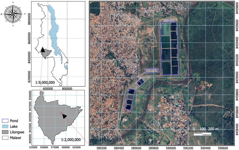
Figure 1. Map of Malawi showing the study area.

Figure 2

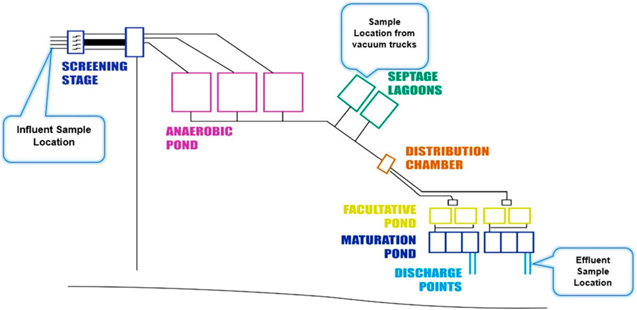
Figure 2. A schematic diagram of the Kauma sewage treatment plant. Not drawn to scale (Adapted with permission from Mtethiwa et al., 2008; Ravina et al., 2021).

Sampling and data collection procedures

The study utilized both secondary and primary data, with a sole focus on domestic sewage. A comprehensive review of documents related to the KSTP produced secondary data. On the other hand, primary data was collected for 30 days from 11 February 2022, to 17 March 2022, twice per day (morning and evening). Wastewater samples were collected systematically from influent raw wastewater, and composite samples were carefully analyzed using standard methods (APHA, 2017; MS682-1:2002, 2002). The pH, COD, total dissolved solids (TDS), total suspended solids (TSS), electrical conductivity (EC), and dissolved oxygen (DO) were all determined. The analyses followed standard methods as prescribed in (APHA, 2017).

Only COD and BOD were determined from samples taken from the Septage lagoon and the effluent-treated wastewater. Samples for the septage lagoon were collected during sludge discharge. To ensure that the samples came from household sources and not from industrial sewage, active attempts were made to consult transporters about the sludge’s origin. Each sludge transportation truck produced four 2-L samples: one at the start, two in the middle, and one at the end. These samples were systematically mixed, with double sampling used to ensure quality assurance and homogeneity.

Self-organizing map

The SOM is typically used as a dimensionality reduction approach that can effectively visualize large datasets. This algorithm is based on unsupervised learning and is entirely data-driven. Self-organizing maps are distinguished by their ability to generate internal representations of various aspects of input signals in a spatially organized and effective manner. As a result, the resulting maps closely resemble or mimic topographically structured maps (Kohonen et al., 1996). They operate in a self-study mode, recognizing patterns and grouping them into groups. As this network cannot measure the meaning of the clusters, the users need to interpret the map in a meaningful and useful manner (Rustum, 2009). Self-organizing maps are inspired by neural networks, which are the foundation of the nervous system. Various philosophies divide the nervous system’s signal progression and network constitution into several categories. In one, nearby neurons in a neural network mutually interact and compete with one another, adapting to become specific detectors of various signal prototypes. The learning is unsupervised or self-organizing in this classification, which serves as the foundation for the development of self-organizing maps.

The main working strategy of such maps is the geometrical transformation of non-linear and complex correlation among high-dimensional data into a relatively simple low-dimensional view. SOM is made up of neurons arranged on standard one or two-dimensional grids, with each neuron, i, represented by an n-dimensional weight/reference/codebook vector given by,

$m_i=\left[m_{i1},...{\mathit{m}}_{\mathit{\text{in}}}\right](1)$

where n is the input vector dimension. These weight vectors comprise the codebook, which depicts the characteristics of the data or process. Figure 3 demonstrates that each neuron has two locations: one in the prototype vector, which is the input space, and another in the map grid, which is the output space (Vesanto et al., 2000a; 2000b). Thus, self-organizing maps are a vector projection method that converts high-dimensional input to low-dimensional output. The connection between adjacent n is determined by the neighborhood relationship.

Figure 3

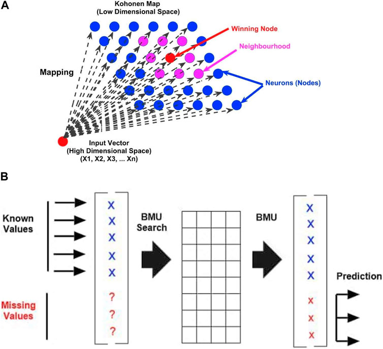
Figure 3. (A) Representation of Winning Node and its neighborhood in Kohonen Self Organizing Map (source: Rustum, 2009). (B) Figure 4: Prediction of missing components of the input vector using the Self-Organizing Map (BMU, Best Matching Unit) (Source: Rustum and Adeloye, 2011b).

The mapping is performed from the input Euclidean data space ${\mathfrak{R}}^n$ to a two-dimensional nodule lattice. Every node $i$ is connected to a unique reference vector $m_i\in R^n$. When there is input data $x\in {\mathfrak{R}}^n$, it is compared to all the $m_i$ to find the best match or response. Input is mapped to specific locations during this process. The Euclidean distance $‖x-m_i‖$, as illustrated in Eq. 2 is used to identify the best matching node, $m_c$, also known as Best Matching Unit as illustrated in Figure 3B (Kangas and Simulation, 2003).

$‖x-m_c‖={\mathit{min}}_i\left\{‖x-m_i‖\right\}(2)$

The basic steps in the development of the map, according to the SOM toolbox developed by the Helsinki University of Technology (Vesanto et al., 2000a), are initialization, training, and validation. Normalization is a process that prevents process variables from having a greater impact than other variables, ensuring that the entire set of variables has the same significance in the construction of maps. Initialization aids the algorithm’s convergence to a good result by assigning weight vector values either randomly or linearly. During this process, each neuron is assigned random weight vectors ranging from zero to one (Vermasvuori et al., 2002). The main goal of training is to find the Best Matching Unit (BMU) or winning node among the map units for each input prototype. This unit is very similar to the input pattern. A distance function is commonly used to measure similarity, with closer distances defining greater similarity as defined by the Euclidean distance function. The best matching unit and its neighboring units are updated to reduce the difference between these units and the input pattern (Hsu, 2006). Two types of algorithms are used for updating: sequential training algorithms and batch training algorithms. Once the best matching unit is identified, its weight vectors are shifted closer to the input vector in the input space, a process known as updating. The best matching unit’s topological neighbor units are also treated in the same way. The size of the adjustment of the weight vector is determined by the distance of these neighborhood neurons or units from the winner output array. More information on training the map can be found in Vesanto et al. (2000a), Lopez Garca and Machon Gonzalez (2004), Rustum (2009).

The SOM’s quality is determined primarily by two error measurements: quantization error (qe) and topographic error (te) (Jorge et al., 2013). The mean Euclidean distance from the input vector to its best matching unit is used to calculate the quantization error.

This, in turn, provides map resolution and aids in identifying outliers. A high quantization error indicates that those input patterns are most likely outliers. The percentage of input vectors for which the best matching unit and the next best are not grid neighbors is referred to as topologic or topographic error. This error indicates the degree of data topology preservation while the map is fitted into the original dataset.

ANFIS

ANFIS modeling is the method of applying various learning techniques developed in the neural network literature to a fuzzy inference system (FIS) (Brown et al., 1994; Brown et al., 1994). The FIS maps its input space to the output space using a fractional non-linear relationship and a set of fuzzy if-then rules (Noori et al., 2013b. A FIS typically has five components: a fuzzification interface, a rule base, a database, a decision-making unit, and a defuzzification interface. One of the most important steps in ANFIS development is the selection of a FIS type. There are various methods for developing the FIS. The first-order Sugeno FIS with two fuzzy rules (Figure 4) is used in this study as given by Eqs 3, 4:

$\text{Rule\hspace{0.17em}}1:\text{If\hspace{0.17em}}x\text{\hspace{0.17em}is\hspace{0.17em}}{\mathrm{A}}_1\text{\hspace{0.17em}and\hspace{0.17em}}y\text{\hspace{0.17em}is\hspace{0.17em}}{\mathrm{B}}_1;\text{\hspace{0.17em}then\hspace{0.17em}}{f}_1=p_{1}x+q_{1}y+r_1(3)$

$\text{Rule\hspace{0.17em}}2:\text{If\hspace{0.17em}}x\text{\hspace{0.17em}is\hspace{0.17em}}{\mathrm{A}}_2\text{\hspace{0.17em}and\hspace{0.17em}}y\text{\hspace{0.17em}is\hspace{0.17em}}{\mathrm{B}}_2;\text{\hspace{0.17em}Then\hspace{0.17em}}{f}_2=p_{2}x+q_{2}y+r_2(4)$

where A₁; A₂ and B₁; B₂ are the membership functions (MFs) for inputs x and y; respectively; and p₁;q₁;r₁ and p₂;q₂;r₂ are the parameters of the output function. Also, the output f is the weighted average of the individual rule outputs. To implement these two rules, an equivalent ANFIS structure (Figure 5) should be developed. In Figure 5, the characteristics of each layer are as follows (Jang, 1993; Lei, 2017).

Figure 4

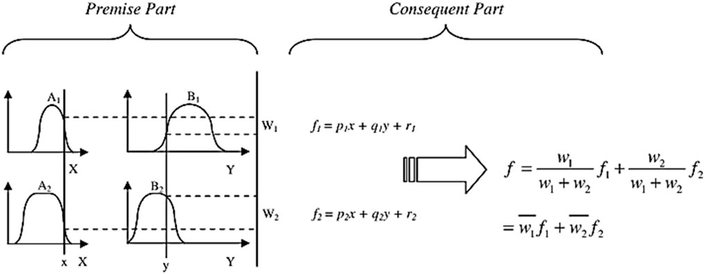
Figure 4. Sugeno’s Fuzzy if-then rule and fuzzy reasoning mechanism (Noori et al., 2013b).

Figure 5

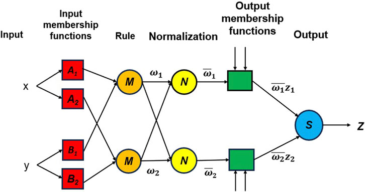
Figure 5. Architecture of ANFIS (Lei, 2017).

Layer 0: It is called the input layer, and has n nodes where n is the number of inputs to the system

Layer 1: Input membership function—The first layer is used to fuzzificate the inputs, and all the nodes of this layer are adaptive. Its outputs are the membership grade of the inputs as given by Eqs 5, 6

$o_i^1=u_{A_i}\left(x\right),i=1,2.(5)$

$o_i^1=u_{B_{i-2}}\left(y\right),i=3,4,(6)$

where $u_{A_i}\left(x\right)$ and $u_{B_{i-2}}\left(y\right)$ are the fuzzy membership functions. Conventionally, the bell-shaped membership function is used, and it is expressed by Eq. 7

$u_{A_i}\left(x\right)=\frac{1}{1+{\left[{\left(\frac{x-c_i}{a_i}\right)}^2\right]}^{b_i}}i=1,2.(7)$

where $a_i$, $b_i$, and $c_i$ are the parameters of the membership functions

Layer 2: Rule—The nodes in this layer are fixed (Not adaptive). These are labeled M to indicate that they play the role of simple multipliers. The outputs of this layer represent the fuzzy strengths $\omega$ of each rule and can be expressed as

$o_1^2={\omega }_i=u_{A_i}\left(x\right)u_{B_i}\left(y\right),i=1,2.(8)$

Layer 3: Normalization—In this layer, the nodes are also fixed. These nodes are labeled with N, which means that they play a normalization role in the fuzzy strengths from the previous layer. The normalization factor is computed by the sum of the weight functions. The outputs of this layer are called normalized fuzzy strengths and are expressed as shown in Eq. 9

$o_i^3=\overline{\omega }i=\frac{{\omega }_i}{{\displaystyle {\sum }_{i=1}^2}{\omega }_i},i=1,2.(9)$

Layer 4: Output membership function—The nodes of this layer are adaptive ones. Its outputs are represented by Eq. 10

$o_i^4=\overline{{\omega }_i}{z}_i=\overline{{\omega }_i}\left(p_{i}x+q_{i}y+r_i\right),i=1,2.(10)$

where $p_i$, $q_i$, $r_i$ are the parameters of the membership functions, respectively.

Layer 5: Output—Only one single fixed node, labeled with S, is in this layer. This node performs the sum of the incoming signals. Thus, the overall output is expressed as shown in Eq. 11.

$o_i^5=z={\displaystyle \sum _{i=1}^2}\overline{{\omega }_i}{z}_i=\frac{{\displaystyle {\sum }_{i=1}^2}{\omega }_i{z}_i}{{\displaystyle {\sum }_{i=1}^2}{\omega }_i}(11)$

Model evaluation criteria

After fitting the input data into ANFIS or any other model, it is important to evaluate how well the model performs. MATLAB offers “goodness of fit” which has a set of parameters that describe the model’s accuracy. Evaluation can be done graphically using residual plots and prediction bounds and numerically using statistical parameters explained below. Graphical measures help the evaluation of the entire dataset at once and can display a wide range of relationships between the model and data (MathWorks, 2020). Numerical evaluation measures include correlation coefficient R, Average Absolute Error (AAE), Mean square error (MSE), and Root Mean Square Error (RMSE). In this study, however, only three indices as given by Eqs 12–14 were used due to their robustness, namely, the correlation coefficient (R) (Wang et al., 2006), the Coefficient of residual mass (CRM) (El-Sadek, 2006), and the Mean percent error (MPE) (Moriasi et al., 2007)

$R=\frac{N{\displaystyle \sum }{O}_i{P}_i-{\displaystyle \sum }{O}_i{\displaystyle \sum }{P}_i}{\sqrt{\left[N{\displaystyle \sum }{O}_i^2-{\left({\displaystyle \sum }{O}_i\right)}^2\right]\left[N{\displaystyle \sum }{P}_i^2-{\left({\displaystyle \sum }{P}_i\right)}^2\right]}}(12)$

$CRM=\frac{{\displaystyle {\sum }_{i=1}^N}{O}_i-{\displaystyle {\sum }_{i=1}^N}{P}_i}{{\displaystyle {\sum }_{i=1}^N}{O}_i}(13)$

$MPE={\displaystyle \sum _{i=1}^N}\left(\frac{\left|O_i-P_i\right|}{Oi}\right)\times 100\%(14)$

where P_i is the predicted value, O_i is the observed value and N is the number of data entries.

The goodness of fit measures the similarity of the shapes of the original and predicted cited time series and ranges between −1 and 1; the absolute value of the correlation coefficient for perfect prediction is unity (Rustum, 2009). The CRM characterizes the tendency to over-estimate CRM < 0 or under-estimate a property (CRM > 0) (Malota et al., 2022) on the other hand, MPE measures the magnitude of errors between the measured and predicted values relative to the measured values. MPE value closer to zero indicates that the predicted values are very close to the measured values (Legates and McCabe, 1999; Malota et al., 2022). To overcome the problem of overfitting, an early stop rule was applied by dividing the KSTP data into three subsets: training (432 data points), validation (92 data sets), and testing (92 data sets).

Ethical consideration

The study sought clearance from the Mzuzu University Research Ethics Committee (MZUNIREC) Ref No: MZUNIREC/DOR/21/62. Permission was also obtained from Lilongwe City Council to engage Laboratory technicians during data collection processes. Informed consent was also obtained from the Laboratory technicians and KSTP who participated in the study.

Results and discussions

Descriptive statistics of Kauma sewage treatment plant data

The preprocessed data, with a sample size of 616 data sets per variable, was examined. The estimated descriptive statistics for a number of variables at the KSTP (Table 1) offered an in-depth overview of influent and effluent characteristics. The pH of the influent wastewater averaged 7.01, indicating slightly alkaline conditions, with a standard deviation (SD) of 0.46, indicating steady pH levels. The upper bound (UB) and lower bound (LB) values (7.05 and 6.97, respectively) set the 95% confidence interval for pH readings. In terms of temperature (Temp inf), the mean of 24.73°C demonstrates a moderate thermal condition, with an SD of 1.83 suggesting variability. UB (24.88) and LB (24.58) determined the 95% confidence interval. BOD₅inf and COD_inf results, with mean values of 228.47 mg/L and 358.34 mg/L, respectively, emphasized the organic load in the influent. TDS_inf and TSS_inf provide information on total dissolved and suspended solids, with values of 465.15 mg/L and 173.28 mg/L, respectively. EC_inf (mean: 783.83 S/cm) and TURB_inf (mean: 9.649 NTU) measurements provided information about electrical conductivity and turbidity. The mean DO_inf of 1.12 mg/L indicated the concentration of dissolved oxygen, which is essential for aerobic living activity. Effluent BOD_5eff (mean: 22.06 mg/L) and COD_eff (mean: 40.41 mg/L) demonstrated a significant reduction in organic and chemical oxygen demand, demonstrating the efficacy of the treatment technology.

Table 1

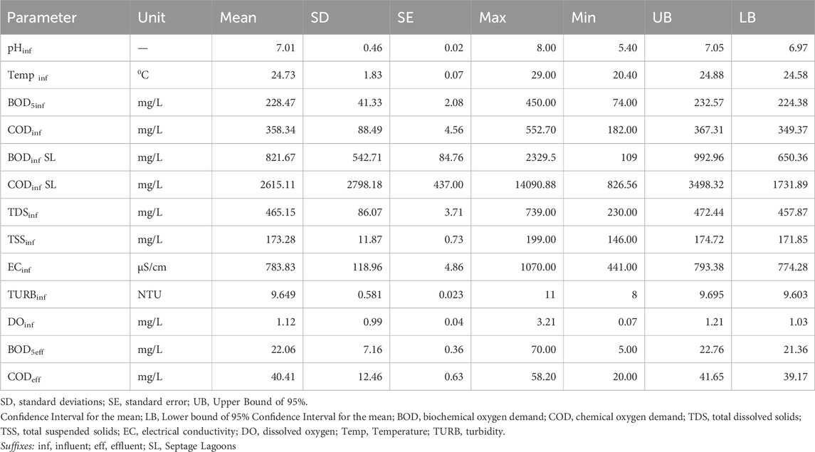
Table 1. Computed descriptive statistics of KSTP data.

The mean COD to BOD₅ ratios were found to be 1.57 and 1.83 for influent and effluent wastewater, respectively. However, samples from septage lagoon had a much higher ratio of 3.18, which is above the average range of 1.25–2.5 for domestic wastewater (Metcalf and Eddy, 2013). This discrepancy stems from various factors as highlighted by Niwagaba et al. (2014). Firstly, wastewater from septic tanks and pit latrines contains more organic and inorganic constituents, such as feces and household chemicals, that can elevate COD levels. In addition, longer retention times in septic tanks and latrines facilitate greater organic decomposition resulting into high COD than BOD₅ levels. Furthermore, anaerobic conditions prevalent in septic tanks produce non-biodegradable compounds that contribute to COD. Lastly there is minimal dilution in septic systems compared to sewered networks, this maintains higher COD concentrations until discharge (Niwagaba et al., 2014).

Before beginning the modeling process, the entire dataset was divided into three sets: the first set of 432 observations was used to train the model, the second set of 92 observations was used to test the model, and the final set of 92 observations was used to validate the model. The study looked at two scenarios: the first consisted of developing an Adaptive Neuro-Fuzzy Inference System (ANFIS) Model from raw data, and the second involved developing a hybrid Self-Organizing Map (SOM) and ANFIS model using extracted features.

SOM component planes

The generation of component planes, a key feature of SOMs, is a rigorous procedure that demonstrates relationships between variables in the data. These planes are created during SOM training, which involves mapping the input space onto a two-dimensional grid of neurons. Each neuron corresponds to a weight vector, whose dimensions match those of the input data (Mng’ombe et al., 2023). By iteratively altering these weights, the SOM learns to represent the data’s underlying structure. Once trained, component planes are created by assigning colors or intensities to neurons based on the values of specified dimensions in the input data (Kumar et al., 2021a). This visualization technique provides useful insights on the relationships and distributions of distinct elements, making it easier to explore and analyze complex datasets (Nkiaka et al., 2016). These component planes, as shown in Figure 6, represent each variable in the SOM. Each plane is effectively a sliced SOM, with a single vector variable indicating its value in each map unit (Kalteh et al., 2008). To improve readability, the component planes are color-filled or grey-scaled, depicting the feature values of each SOM unit inside the 2-D lattice. Darker hues imply that the associated variable component has a lower relative value. This visual depiction efficiently delineates zones where a variable is high, low, or average, allowing for a simple understanding of the correlation between SOM-simulated values of selected wastewater parameters (Kumar et al., 2021b).

Figure 6

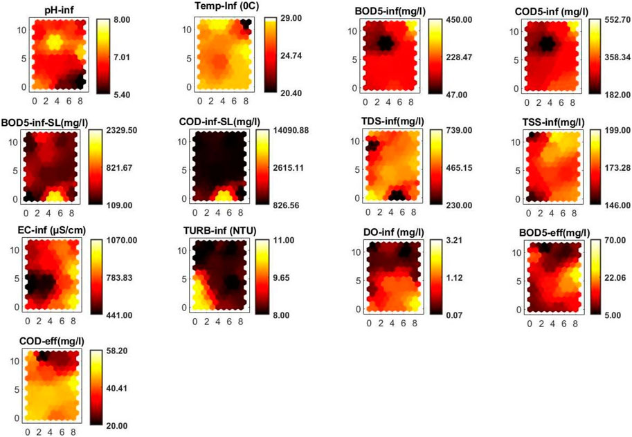
Figure 6. SOM component planes.

A visual analysis of the component planes indicates that the BOD_5inf plane’s color (or gray) gradient aligns parallel to the COD_inf gradient, demonstrating a correlation where high BOD_5inf values are associated with high COD_inf values and vice versa. Similarly, greater BOD_5eff levels correlate with high COD_eff levels and vice versa. The component planes support a negative association between pH and BOD₅inf, CODi_nf, and DO_inf, with low pH values associated with high BOD_5inf, COD_inf, and DO_inf values. The expected positive association between BOD and COD has been validated, correlating with expectations that COD values are often greater than BOD values, with the ratio fluctuating depending on wastewater characteristics (Rai et al., 2019). The entire correlation matrix containing all 11 variables of the prototype vectors is shown in Table 2. While this table is a simple tool for examining the linear relationships between different variables, its findings are consistent with the cross-correlation indications derived from the much more complex SOM analysis, which resulted in the development of the component planes.

Table 2

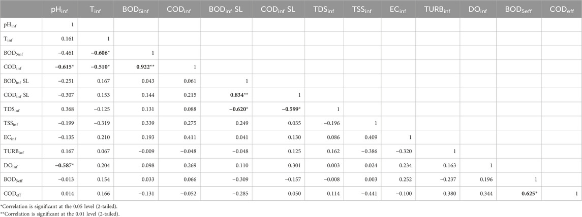
Table 2. Correlation matrix for variables in code vectors.

Table 2 presents a thorough perspective of the correlation matrix for the variables within the code vectors, giving insights into the complex relationships between different parameters within the wastewater treatment framework. Among the notable findings was a modest positive correlation between pH and temperature (T_inf), indicating a minor tendency for both variables to fluctuate together. Furthermore, a strong negative connection occurred between influent BOD_5inf and CODi_nf, which corresponded to the expected inverse association in wastewater. The component planes revealed the influence of the septage lagoon (BOD_inf SL and COD_inf SL) on numerous parameters, demonstrating a complicated interaction between the septage lagoon and other wastewater properties. Positive correlations between total dissolved solids (TDS_inf) and total suspended solids (TSS_inf) in the influent indicated a simultaneous increase in both metrics. In contrast, electrical conductivity (EC_inf) exhibited a negative relationship with turbidity (TURB_inf), implying that higher electrical conductivity is associated with clearer wastewater. DO_inf (dissolved oxygen in influent) had a substantial negative correlation with effluent biochemical oxygen demand (BOD_5eff), highlighting the relevance of dissolved oxygen in the treatment process. Furthermore, effluent chemical oxygen demand (COD_eff) demonstrated a positive association with TSS_inf, indicating a possible relationship between suspended solids concentration and chemical oxygen demand in effluent. In conclusion, our correlation matrix gave a foundational understanding of the interplay of several wastewater metrics, stressing the importance of these correlations in describing wastewater quality, as highlighted by the significant correlations at the 0.05 and 0.01 levels.

ANFIS model structure

Table 3 displays the model architectures of several models developed and evaluated with Gaussian membership functions. Multiple models were developed by experimenting with different combinations of input variables and using various membership functions. The association of these input factors to effluent BOD₅ and the promptness with which each variable could be measured influenced their selection. Given the available database, the inclusion of four input variables was assessed to be the maximum number of combinations possible. For example, when using four inputs, each associated with three membership functions, the total number of adjusted parameters, as calculated by Eq. 15, was 430—well within the 432 data points available for training. The evaluation of five parameters, however, using five parameters could exceed the number of training data sets, limiting the model’s degrees of freedom.

$N_{total}=\left(N_{input}\times N_{mf}\times N_{pp}\right)+\left(l\times N_{cp}\right)(15)$

$l={\left(N_{mf}\right)}^{N_{input}}(16)$

$N_{cp}=N_{input}+1(17)$

where $N_{total}$ is the total number of modified parameters, $N_{input}$ is the number of inputs, $N_{mf}$ is the number of membership functions associated with each input, $N_{pp}$ is the number of modified parameters per membership function, i. e., in the case of the Gaussian membership function; $l$ in Eq. 16 is the number of rules; $N_{cp}$ in Eq. 17 is the number of modified parameters in the sequence part of each rule

Table 3

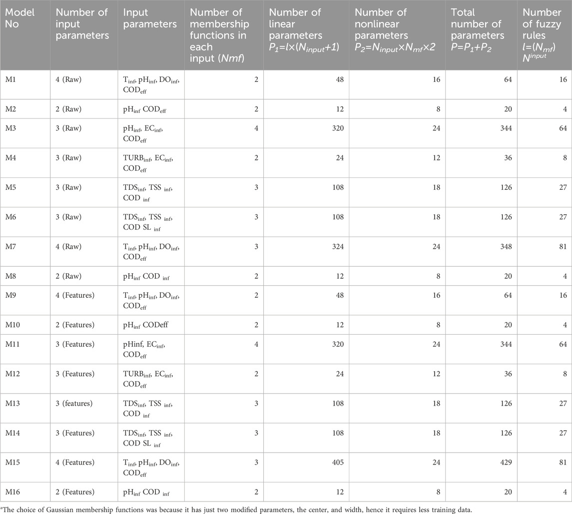
Table 3. The structure of the ANFIS models developed and tested in the study for predicting effluent BOD values using Gaussian membership functions^a.

Table 4 presents a detailed summary of the performance of produced models in two scenarios: M1–M8, where models were built using raw data, and M9–M16, where models were built using extracted features using SOM. The results show that model M1–M16’s performance was unsatisfactory, as shown by higher values of the Coefficient of Residual Mass (CRM) and Mean Percent Errors (MPE). Furthermore, as seen in Table 5, models developed utilizing raw data produced negative results.

Table 4

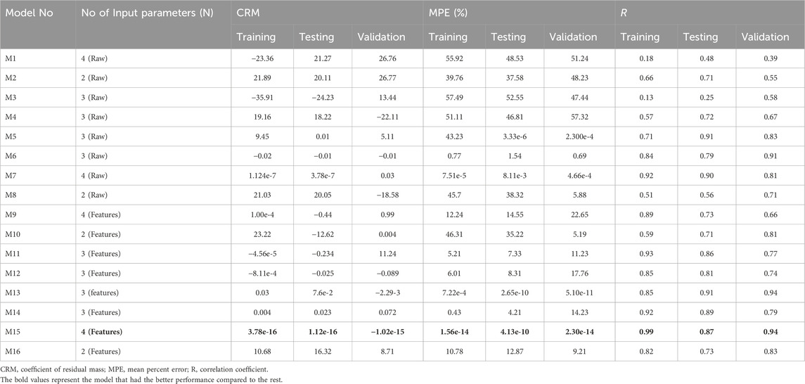
Table 4. The performance of the ANFIS models to predict BOD₅.

Table 5

Table 5. Statistics summary of the ANFIS models to predict effluent BOD₅.

Table 4 shows that improving the raw data by pre-processing with the SOM technique considerably improved model performance. Consider models 7 and 15, which both had the same structure—four inputs and three membership functions associated with each input. However, model number 15 outperformed model number 7, with the correlation coefficient in the validation dataset increasing from 0.81 to 0.94. This trend is repeated for the remaining models, demonstrating the effectiveness of raw data pre-processing with the SOM algorithm in enhancing overall model performance.

The ANFIS models’ performance, as presented in Tables 4, 5, provides a more comprehensive understanding of the predictive abilities for BOD₅ concentrations. The coefficient of residual mass (CRM), mean percent error (MPE), and correlation coefficient for models with raw and extracted features are presented in Table 4. Model M1, which had four raw input parameters, had negative CRM values during testing and validation, indicating a probable model fitting issue. Similarly, during testing, Model M5 demonstrated an MPE close to zero, indicating a near-perfect match. Models M3 and M11, which used three raw input parameters, had negative CRM values, indicating an overestimation of BOD₅ concentrations. The addition of feature extraction in Models M9–M16 significantly increased performance, with the Model M15 exhibiting excellent results including nearly minimal CRM and MPE values and excellent correlation coefficients.

Table 5 summarizes statistics on predicted effluent BOD₅ concentrations, which offer light on the models’ ability to mimic observed values. Models containing raw input parameters, such as M3 and M4, had broader ranges and higher mean values, indicating difficulties in predicting extreme concentrations. Model M5 stood out for its consistency with observed values, having a shorter range and closer mean value alignment. Models M9–M16, on the other hand, demonstrated competitive performance with reduced ranges and mean values by leveraging extracted characteristics. Model M15, in particular, displayed distinct match with observed values. However, negative predictions in raw data, as demonstrated in Models M2 and M8, should be taken into account because they may reflect limits in effectively capturing complex relationships. Overall, the introduction of feature extraction demonstrated potential to enhance the predicted accuracy of ANFIS models for effluent BOD₅ values.

These findings are consistent with previous research, as shown in Table 6, and highlight the need of combining ANFIS algorithms with complementing approaches such as SOM to improve model accuracy. Discrepancies discovered in similar studies highlight the complexities of this methodology and its critical role in improving the reliability and overall performance of ANFIS models.

Table 6

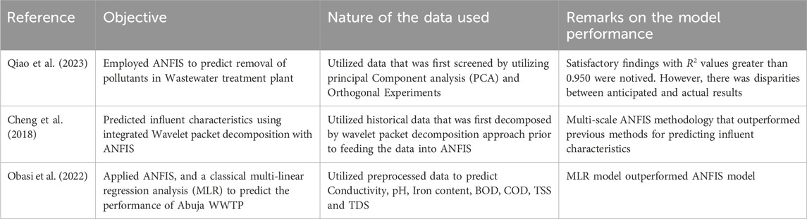
Table 6. Comparative studies in utilization of ANFIS for optimization problems.

Given Model 15’s higher performance as compared to its competitors, an in-depth scrutiny was conducted solely on this model. Model 15 is distinguished by three membership functions associated with each of its four input variables, namely, T_inf, pH_inf, DO_inf, and COD_eff, as illustrated in Figures 7, 8. Figure 9 depicts the membership functions and Gaussian membership functions based on the operational range of the model.

Figure 7

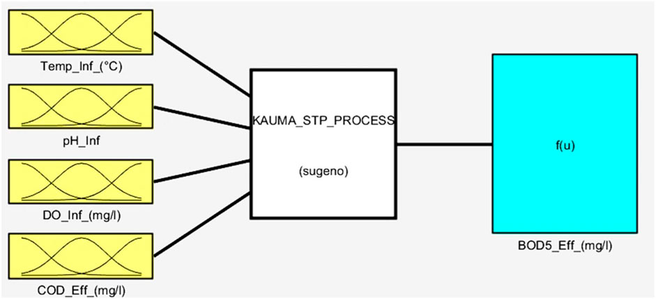
Figure 7. The structure of Model number 15.

Figure 8

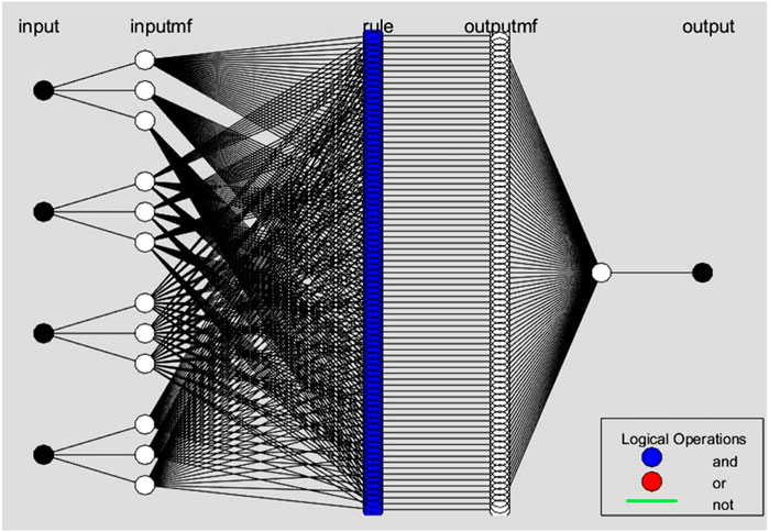
Figure 8. Schematic diagram of Model number 15 with 3 membership functions and 81 “IF -THEN” rules.

Figure 9

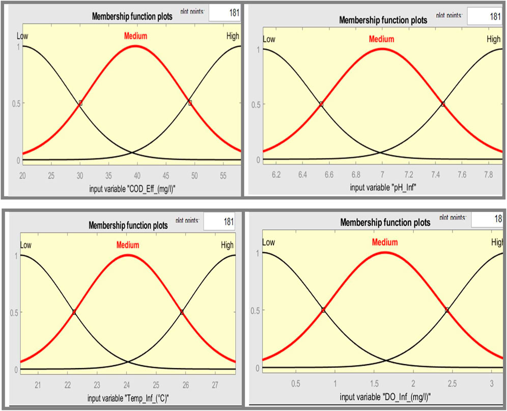
Figure 9. Fuzzy membership Functions in the input space.

Membership functions play an important role in defining and expressing the fuzzy sets that are essential to a fuzzy inference system. Figures 7–9 exemplify how these functions help to express fuzzy thinking and decision-making based on linguistic considerations. Membership functions, in essence, quantify the degree to which an input value aligns with a given fuzzy set. These functions, which typically span a specific range of input values, assign a membership degree, ranging from 0 to 1, to each value inside that range. This degree of membership indicates the input value’s association with the given fuzzy set, providing a deeper understanding of the input’s participation in the larger fuzzy set.

The parameters for the Gaussian membership functions related to input variables are summarized in Table 7, which includes the center (c) and width (b) components. The developed model is distinguished by a thorough set of 81 rules that comprise a total of 429 modified parameters. There are 24 non-linear parameters among these, with the remaining 405 linear parameters forming the model’s complicated framework.

Table 7

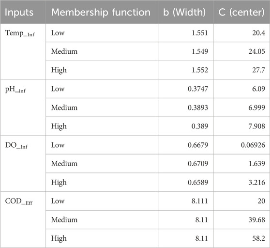
Table 7. The parameters of Gaussian membership functions associated with input variables.

Table 8 illustrates the optimized fuzzy rules that govern Model 15. These 81 rules define the complex relationships between input and output variables. Figure 10 illustrates the integration process of these rules, which complements this tabular representation. Table 8 systematically details each rule, with discrete parts dedicated to the “IF and THEN” conditions for each rule. The IF component defines a set of criteria depending on input variables, whereas the THEN component defines the expected consequence or action. For example, rule 1 in Table 8 can be understood as follows:

Table 8

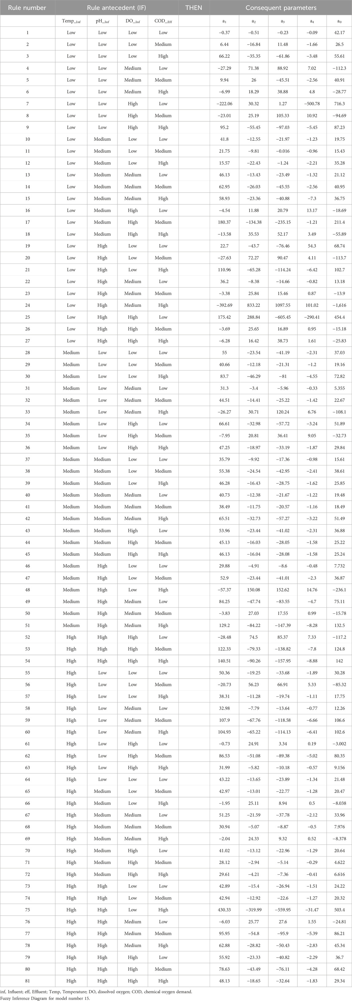
Table 8. Optimised fuzzy rules generated using modeling strategy developed in this study for model number 15.

Figure 10

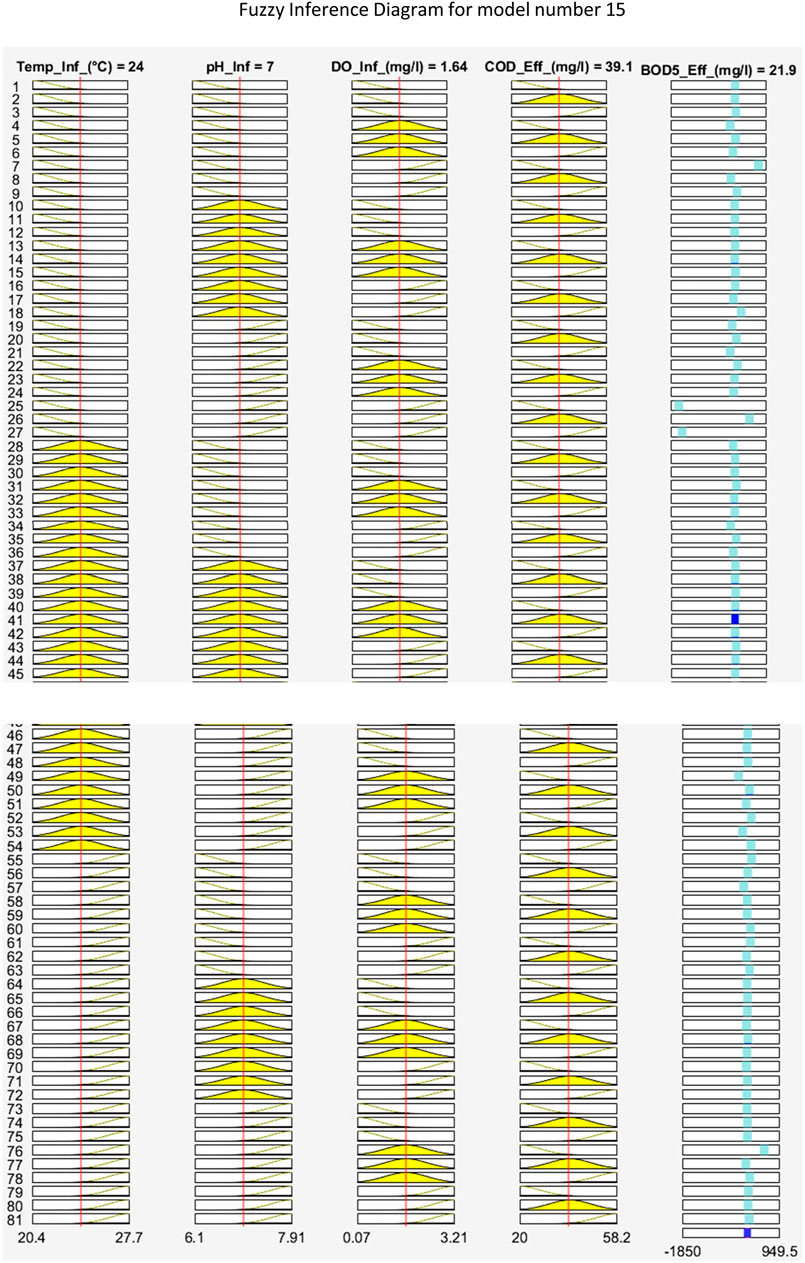
Figure 10. (Continued).

IF (TEMP) is Low and (pH) is Low and (DO_inf) is Low and COD_eff is low, THEN (effluent BOD) is 42.17 - (0.37*temp) - (0.51* pH) - (0.23*DO) -(0.09*COD_eff)

Data that was not used in the training phase was used for testing and validation of the trained model. Figures 11–13 depict time series plots of observed and anticipated effluent BOD₅ alongside their corresponding residuals during the training, testing, and validation processes. Figure 14 depicts the modeled data in comparison to the observed data during the training, testing, and validation phases.

Figure 11

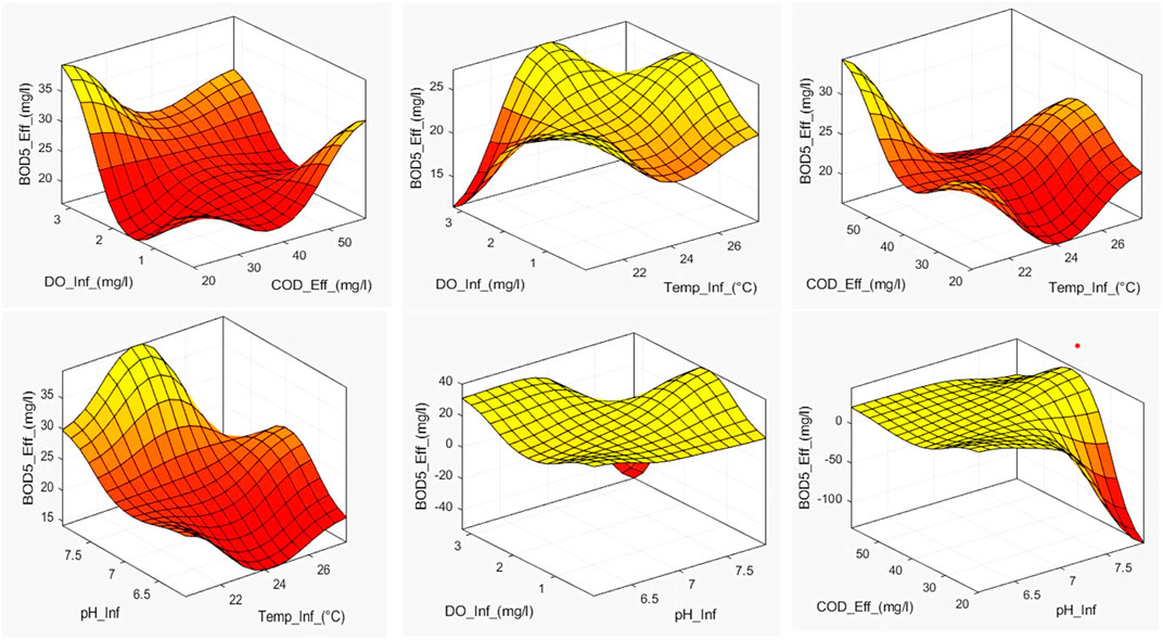
Figure 11. Graphical user interface of model number 15. Contrary to Figure 10, To obtain the output value as shown in the picture, the user only needs to enter the input values.

Figure 12

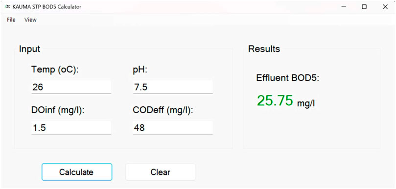
Figure 12. Time series plots of observed and predicted BOD during training for model number 15.

Figure 13

Figure 13. Time series plots of observed and predicted BOD during testing for model number 15.

Figure 14

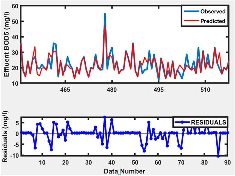
Figure 14. Time series plots of observed and predicted BOD during Validation for model number 15.

To determine the number of rules, the typical fuzzy inference approach relies on an expert judgment which is well-versed in the simulated system. This expert employs heuristic insights gained from vast experience gained from the simulations. In this study, however, the number of membership functions allocated to each input variable was established empirically by trial and error, eliminating the requirement for an expert judgement. The suggested model accurately determines process conditions by combining values from multiple factors. Furthermore, the suggested model is resistant to missing variables and outliers. In comparison to deterministic models, creating a fuzzy logic model is likewise a relatively simple task.

The interactions between numerous input variables and a single output variable are frequently shown via 3D graphs when using the Fuzzy Toolbox in MATLAB. These graphs support decision-making and aid in understanding fuzzy systems’ behavior. To understand a 3D graph produced by the Fuzzy Toolbox, it is necessary to examine its shape, contours, and surface properties. As illustrated in Figure 15 the model input variables (Temp__Inf, pH__Inf, DO__inf, and COD__eff) are represented on the X and Y-axes of the graphs. These variables frequently match up with linguistic concepts or membership algorithms specified in the fuzzy system. For interpretation, it is crucial to comprehend the range and linguistic significance of these variables. On the 3D graph’s Z-axis, the output variable (BOD₅__eff) is shown. It displays the system’s reaction or output to the supplied inputs. On the graph, the output variable values are typically depicted by color or contour lines.

Figure 15

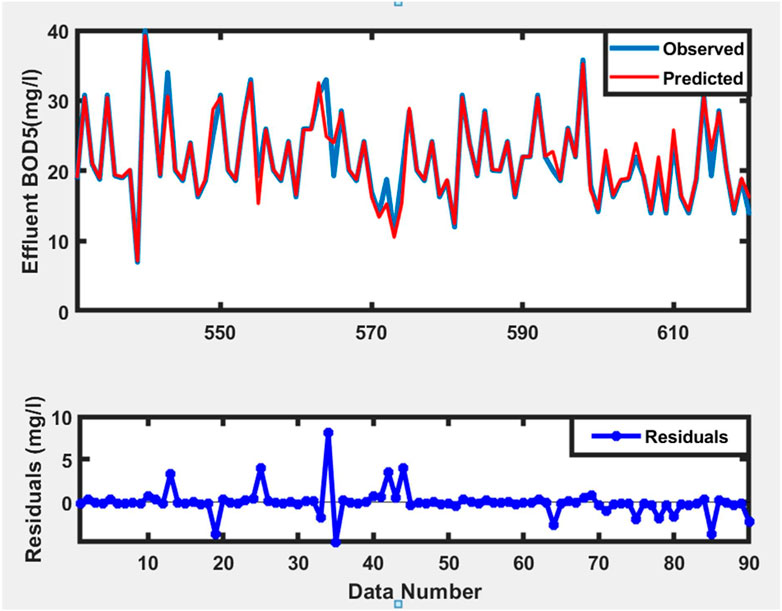
Figure 15. The scatter plot of modeled versus observed data during training, testing, and validation for model number 15.

Conclusion

The current study offers a novel approach for predicting BOD₅ values in wastewater using wastewater data collected from the KSTP in Lilongwe City. To successfully predict effluent BOD₅, the hybrid SOM-ANFIS model was trained, validated, and tested. Initially, a set of measured raw data was used to train and test the ANFIS model. The model did not work well, though, because the raw data was noisy. To tackle this issue, features from the data were extracted using the SOM. These retrieved features were used to train and evaluate a new set of models, thereby improving their performance. The results showed that the SOM-ANFIS model outperformed the ordinary ANFIS model in terms of modeling capabilities and certainty, even when accounting for varying numbers of inputs and fuzzy membership functions. The SOM-ANFIS model was also able to handle blank spaces in the data or missing values without challenges. This implies that SOM assisted models have greater capabilities compared to ordinary ANFIS in predicting BOD₅ for KSTP. Using MATLAB’s app designer, an easy-to-use graphical user interface as demonstrated in Figure 16 was developed to improve usability and user-friendliness. The developed GUI was able to facilitate user interaction and understanding the created fuzzy inference system. The developed model is expected to reduce treatment operation and testing costs, allow continuous monitoring, and consequently protect the environment. Future improvement of the developed model will include integrating it with hardware components through the Supervisory Control and Data Acquisition (SCADA) system. The authors recommend for the development of a specialized model, such as a Convolutional Neural Network, intended exclusively for fecal sludge characterization. Considering the fact that faecal sludge characteristics are highly variable with space and time, it is further recommended that data from other sources such as rivers and other wastewater treatment facilities in Malawi and beyond be collected to update the developed models. This will widen the application of developed models to expose them to a wider range of scenarios.

Figure 16

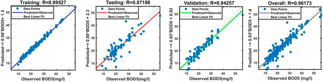
Figure 16. 3D response graphs for model number 15.

Software availability statement

The SOM Toolbox (Version 2.2) for MATLAB used in this study is freely available for download from GitHub (https://github.com/ilarinieminen/SOM-Toolbox). The study also used the fuzzy logic toolbox available in MATLAB

Data availability statement

The original contributions presented in the study are included in the article/supplementary material, further inquiries can be directed to the corresponding author.

Author contributions

MHM: Conceptualization, Data curation, Formal Analysis, Funding acquisition, Investigation, Methodology, Project administration, Resources, Visualization, Writing–original draft, Writing–review and editing. EM: Conceptualization, Data curation, Investigation, Methodology, Software, Supervision, Writing–original draft, Writing–review and editing, Formal Analysis, Funding acquisition, Project administration, Resources, Validation, Visualization. BC: Project administration, Supervision, Writing–original draft, Writing–review and editing. RC: Writing–original draft, Writing–review and editing, Methodology.

Funding

The authors declare that financial support was received for the research, authorship, and/or publication of this article. This work received funding from National Commission for Science and Technology (NCST) under NCST Small Grants Scheme. It also received funding from the Malawi Ministry of Education, Science, and Technology under Higher Education Research and Development for Young Researchers (postgraduate) scheme (Ref. No. EDU/HE/21/74).

Acknowledgments

The Authors are grateful to the following people, Dr. Linda Strande (Ph.D.) and the entire team from Eawag (Swiss Federal Institute of Aquatic Science and Technology) for the technical guidance and material support. Lilongwe City Council for the support rendered during data collection, particularly to the following people Eng. Phyllis Mkwezalamba, Mr. Obvious Nyirenda, Mr. John Thyoka, Mr. Chimango Mweso, and Mr. Orymo Nyirenda

Conflict of interest

The authors declare that the research was conducted in the absence of any commercial or financial relationships that could be construed as a potential conflict of interest.

Publisher’s note

All claims expressed in this article are solely those of the authors and do not necessarily represent those of their affiliated organizations, or those of the publisher, the editors and the reviewers. Any product that may be evaluated in this article, or claim that may be made by its manufacturer, is not guaranteed or endorsed by the publisher.

References

Abunama, T., Othman, F., Ansari, M., and El-Shafie, A. (2019). Leachate generation rate modeling using artificial intelligence algorithms aided by input optimization method for an MSW landfill. Environ. Sci. Pollut. Res. 26 (4), 3368–3381. doi:10.1007/s11356-018-3749-5

PubMed Abstract | CrossRef Full Text | Google Scholar

Alsulaili, A., and Refaie, A. (2021). Artificial neural network modeling approach for the prediction of five-day biological oxygen demand and wastewater treatment plant performance. Water Supply 21 (5), 1861–1877. doi:10.2166/WS.2020.199

CrossRef Full Text | Google Scholar

APHA (2017). Standard methods for the examination of water and wastewater. Washington, D.C., USA: American Public Health Association.

Google Scholar

Arlyapov, V. A., Plekhanova, Y. V., Kamanina, O. A., Nakamura, H., and Reshetilov, A. N. (2022). Microbial biosensors for rapid determination of biochemical oxygen demand: approaches, tendencies and development prospects. Biosensors 12 (10), 842. doi:10.3390/BIOS12100842

PubMed Abstract | CrossRef Full Text | Google Scholar

Bekkari, N., and Zeddouri, A. (2019). Using artificial neural network for predicting and controlling the effluent chemical oxygen demand in wastewater treatment plant. Manag. Environ. Qual. Int. J. 30 (3), 593–608. doi:10.1108/meq-04-2018-0084

CrossRef Full Text | Google Scholar

Brown, M., Harris, C. J., and Christopher, J. (1994). Neurofuzzy adaptive modelling and control. Hoboken, New Jersey, USA: Prentice Hall.

Google Scholar

Cheng, Z., Li, X., Bai, Y., and Li, C. (2018). Multi-scale fuzzy inference system for influent characteristic prediction of wastewater treatment. Clean. – Soil, Air, Water 46 (7), 1700343. doi:10.1002/CLEN.201700343

CrossRef Full Text | Google Scholar

El Alaoui El Fels, A., Mandi, L., Kammoun, A., Ouazzani, N., Monga, O., and Hbid, M. L. (2023). Artificial intelligence and wastewater treatment: a global scientific perspective through text mining. WaterSwitzerl. 15 (19), 3487. doi:10.3390/w15193487

CrossRef Full Text | Google Scholar

El-Sadek, A. (2006). Upscaling field scale hydrology and water quality modelling to catchment scale. Water Resour. Manag. 21 (1), 149–169. doi:10.1007/S11269-006-9046-Y

CrossRef Full Text | Google Scholar

Hassen, E. B., and Asmare, A. M. (2018). Predictive performance modeling of habesha brewery’s wastewater treatment plant using artificial neural networks. J. Environ. Treat. Tech. 6 (2), 15–25.

Google Scholar

Hsu, C.-C. (2006). Generalizing self-organizing map for categorical data. IEEE Trans. Neural Netw. 17 (2), 294–304. doi:10.1109/TNN.2005.863415

PubMed Abstract | CrossRef Full Text | Google Scholar

Jang, J. S. R. (1993). ANFIS: adaptive-network-based fuzzy inference system. IEEE Trans. Syst. Man Cybern. 23 (3), 665–685. doi:10.1109/21.256541

CrossRef Full Text | Google Scholar

Kalteh, A. M., Hjorth, P., and Berndtsson, R. (2008). Review of the self-organizing map (SOM) approach in water resources: analysis, modelling and application. Environ. Model. Softw. 23 (7), 835–845. doi:10.1016/J.ENVSOFT.2007.10.001

CrossRef Full Text | Google Scholar

Kangas, J., and Kohonen, T. (1996). Developments and applications of the self-organizing map and related algorithms. Math. Comput. Simul. 41, 3–12. doi:10.1016/0378-4754(96)88223-1

CrossRef Full Text | Google Scholar

Karami, H., DadrasAjirlou, Y., Jun, C., Bateni, S. M., Band, S. S., Mosavi, A., et al. (2022). A novel approach for estimation of sediment load in dam reservoir with hybrid intelligent algorithms. Front. Environ. Sci. 10, 821079. doi:10.3389/fenvs.2022.821079

CrossRef Full Text | Google Scholar

Karube, I., Matsunaga, T., Mitsuda, S., and Suzuki, S. (1977). Microbial electrode BOD sensors. Biotechnol. Bioeng. 19 (10), 1535–1547. doi:10.1002/BIT.260191010

PubMed Abstract | CrossRef Full Text | Google Scholar

Kohonen, T., Hynninen, J., Kangas, J., and Laaksonen, J. (1996). SOM_PAK: the self-organizing map program package. Available at: http://citeseerx.ist.psu.edu/viewdoc/download?doi=10.1.1.455.8698&rep=rep1&type=pdf.

Google Scholar

Kumar, N., Rustum, R., Shankar, V., and Adeloye, A. J. (2021a). Self-organizing map estimator for the crop water stress index. Comput. Electron. Agric. 187, 106232. doi:10.1016/J.COMPAG.2021.106232

CrossRef Full Text | Google Scholar

Kumar, N., Shankar, V., Rustum, R., and Adeloye, A. J. (2021b). Evaluating the performance of self-organizing maps to estimate well-watered canopy temperature for calculating crop water stress index in Indian Mustard (Brassica Juncea). J. Irrigation Drainage Eng. 147 (2), 4020040. doi:10.1061/(ASCE)IR.1943-4774.0001526

CrossRef Full Text | Google Scholar

Legates, D. R., and McCabe, G. J. (1999). Evaluating the use of “goodness-of-fit” Measures in hydrologic and hydroclimatic model validation. Water Resour. Res. 35 (1), 233–241. doi:10.1029/1998WR900018

CrossRef Full Text | Google Scholar

Lei, Y. (2017). Individual intelligent method-based fault diagnosis. Intelligent Fault Diagnosis Remain. Useful Life Predict. Rotating Mach., 67–174. doi:10.1016/B978-0-12-811534-3.00003-2

CrossRef Full Text | Google Scholar

Lin, W., Hanyue, Y., and Bin, L. (2022). Prediction of wastewater treatment system based on deep learning. Front. Ecol. Evol. 10, 1064555. doi:10.3389/fevo.2022.1064555

CrossRef Full Text | Google Scholar

Liu, Y., Li, J., Wan, N., Fu, T., Wang, L., Li, C., et al. (2020). A current sensing biosensor for BOD rapid measurement. Archaea 2020, 1–7. doi:10.1155/2020/8894925

PubMed Abstract | CrossRef Full Text | Google Scholar

Lopez Garcia, H., and Machon Gonzalez, I. (2004). Self-organizing map and clustering for wastewater treatment monitoring. Eng. Appl. Artif. Intell. 17 (3), 215–225. doi:10.1016/J.ENGAPPAI.2004.03.004

CrossRef Full Text | Google Scholar

Malota, M., Mchenga, J., and Chunga, B. A. (2022). WaSim model for subsurface drainage design using soil hydraulic parameters estimated by pedotransfer functions. Appl. Water Sci. 12 (7), 171–211. doi:10.1007/S13201-022-01699-Z

CrossRef Full Text | Google Scholar

Mathsworks (2020). MATLAB:Getting started Guide (R2020a ed.). Available at: https://www.mathworks.com/products/matlab/getting-started.html.

Google Scholar

Metcalf & Eddy (2013). Wastewater engineering: treatment and resource recovery. Available at: https://books.google.com.cu/books?id=6KVKMAEACAAJ.

Google Scholar

Mng’ombe, M. H., Chunga, B. A., Mtonga, E. W., Chidya, R. C. G., and Malota, M. (2023). Infilling missing data and outliers for a conventional sewage treatment plant using a self-organizing map: a case study of Kauma Sewage Treatment Plant in Lilongwe, Malawi. H2Open J. 6 (2), 280–296. doi:10.2166/H2OJ.2023.013

CrossRef Full Text | Google Scholar

Mohanty, S., Patra, P. K., Mohanty, A., Harrag, A., and Rezk, H. (2022). Adaptive neuro-fuzzy approach for solar radiation forecasting in cyclone ravaged Indian cities: a review. Front. Energy Res. 10, 828097. doi:10.3389/fenrg.2022.828097

CrossRef Full Text | Google Scholar

Moriasi, D., Arnold, J. G., Van Liew, M. W., Bingner, R. L., Harmel, R. D., and Veith, T. L. (2007). Model evaluation guidelines for systematic quantification of accuracy in watershed simulations. Trans. ASABE 50 (3), 885–900. doi:10.13031/2013.23153

CrossRef Full Text | Google Scholar

MS682-1:2002 (2002). Water quality sampling. Part 1:Guidance on the design, and sampling programs and sampling techniques-. Malawi Bureau Stand. Vol. Part 1, 23.

Google Scholar

Mtethiwa, A., Munyenyembe, A., Jere, W., and Nyali, E. (2008). Efficiency of oxidation ponds in wastewater treatment. Int. J. Environ. Res. 2 (2), 149–152.

Google Scholar

Niwagaba, C. B., Mbeguere, M., and Strande, L. (2014). Faecal sludge quantification, characterisation and treatment objectives. Faecal Sludge Manag. 35.

Google Scholar

Nkiaka, E., Nawaz, N. R., and Lovett, J. C. (2016). Using self-organizing maps to infill missing data in hydro-meteorological time series from the Logone catchment, Lake Chad basin. Environ. Monit. Assess. 188 (7), 400–412. doi:10.1007/S10661-016-5385-1

PubMed Abstract | CrossRef Full Text | Google Scholar

Noori, R., Safavi, S., and Nateghi Shahrokni, S. A. (2013a). A reduced-order adaptive neuro-fuzzy inference system model as a software sensor for rapid estimation of five-day biochemical oxygen demand. J. Hydrology 495, 175–185. doi:10.1016/J.JHYDROL.2013.04.052

CrossRef Full Text | Google Scholar

Noori, R., Safavi, S., and Nateghi Shahrokni, S. A. (2013b). A reduced-order adaptive neuro-fuzzy inference system model as a software sensor for rapid estimation of five-day biochemical oxygen demand. J. Hydrology 495, 175–185. doi:10.1016/J.JHYDROL.2013.04.052

CrossRef Full Text | Google Scholar

Obasi, P. O., Ismail I, A., Abdulazeez, R., Najashi, B. ’u G., Jibril, M., Awaisu Shafiu, I., et al. (2022). Performance analysis and control of wastewater treatment plant using Adaptive Neuro-Fuzzy Inference System (ANFIS) and Multi-Linear Regression (MLR) techniques. GSC Adv. Eng. Technol. 4 (2), 001–016. doi:10.30574/GSCAET.2022.4.2.0033

CrossRef Full Text | Google Scholar

Okeke, O. P., Ismail, I. A., Abdulazeez, R., Bara’u, G. N., M.M, J., Awaisu, S. I., et al. (2022). Performance analysis and control of wastewater treatment plant using Adaptive Neuro-Fuzzy Inference System (ANFIS) and Multi-Linear Regression (MLR) techniques. GSC Adv. Eng. Technol. 4 (2), 001–016. doi:10.30574/GSCAET.2022.4.2.0033

CrossRef Full Text | Google Scholar

Pitman, K., Raud, M., and Kikas, T. (2015). Biochemical oxygen demand sensor arrays. Agron. Res. 13 (2), 382–395.

Google Scholar

Pourzangbar, A., Jalali, M., and Brocchini, M. (2023). Machine learning application in modelling marine and coastal phenomena: a critical review. Front. Environ. Eng. 2, 1235557. doi:10.3389/FENVE.2023.1235557

CrossRef Full Text | Google Scholar

Qiao, L., Yang, P., Leng, Q., Xu, L., Bi, Y., Xu, J., et al. (2023). Exploring ANFIS application based on actual data from wastewater treatment plant for predicting effluent removal quality of selected major pollutants. J. Water Process Eng. 56, 104247. doi:10.1016/J.JWPE.2023.104247

CrossRef Full Text | Google Scholar

Rai, A., Singh, S., Zia, S., Manikpuri, P., and Alexander, K. (2019). Relation between COD and BOD in Sangam water samples for pre and post bath during Kumbh. Available at: https://www.entomoljournal.com/archives/2019/vol7issue3/PartS/7-3-187-712.pdf.

Google Scholar

Ramos, M. J. C., Gonzalez, I. M., Garcia, H. L., Rolle, J. L. C., Leal, E. C., Loff, M., et al. (2013). “Visual supervision of a waste water biological reactor using artificial intelligence algorithms,” in 2013 International Conference on New Concepts in Smart Cities: Fostering Public and Private Alliances (SmartMILE), Gijon, Spain, December, 2013.

CrossRef Full Text | Google Scholar

Ravina, M., Galletta, S., Dagbetin, A., Kamaleldin, O. A. H., Mng’ombe, M., Mnyenyembe, L., et al. (2021). Urban wastewater treatment in african countries: evidence from the hydroaid initiative. Sustainability 13 (22), 12828. doi:10.3390/SU132212828

CrossRef Full Text | Google Scholar

Rustum, R. (2009). Modelling activated sludge wastewater treatment plants using artificial intelligence techniques (fuzzy logic and neural networks). Available at: https://www.ros-test.hw.ac.uk/xmlui/handle/10399/2207.

Google Scholar

Rustum, R., and Adeloye, A. (2011a). “Artificial intelligence modeling of wastewater treatment plants: theory, applications and limitations,” in VDM verlag Dr. Muller (Saarbrücken, Germany: OmniScriptum).

Google Scholar

Rustum, R., and Adeloye, A. (2011b). “Artificial intelligence modeling of wastewater treatment plants: theory, applications and limitations,” in VDM verlag Dr. Muller (Saarbrücken, Germany: OmniScriptum).

Google Scholar

Vázquez, R. F., Feyen, L., Feyen, J., and Refsgaard, J. C. (2002). Effect of grid size on effective parameters and model performance of the MIKE-SHE code. Hydrol. Process. 16 (2), 355–372. doi:10.1002/HYP.334

CrossRef Full Text | Google Scholar

Vermasvuori, M., Endén, P., Haavisto, S., and Jämsä-Jounela, S. L. (2002). “The use of Kohonen self-organizing maps in process monitoring,” in 1st International IEEE Symposium, Varna, Bulgaria, September, 2002, 2–7.

Google Scholar

Vesanto, J., Himberg, J., Alhoniemi, E., and Parhankangas, J. (2000a). SOM toolbox for Matlab 5. Available at: https://citeseerx.ist.psu.edu/viewdoc/download?doi=10.1.1.25.7561&rep=rep1&type=pdf.

Google Scholar

Vesanto, J., Himberg, J., Alhoniemi, E., and Parhankangas, J. (2000b). SOM toolbox for matlab 5 libella oy espoo 2000 SOM toolbox for matlab 5. Available at: http://www.cis.hut./projects/somtoolbox/http://www.cis.hut./projects/somtoolbox/.

Google Scholar

Wang, X., Mosley, C. T., Frankenberger, J. R., and Kladivko, E. J. (2006). Subsurface drain flow and crop yield predictions for different drain spacings using DRAINMOD. Agric. Water Manag. 79 (2), 113–136. doi:10.1016/J.AGWAT.2005.02.002

CrossRef Full Text | Google Scholar

Ward, B. J., Andriessen, N., Tembo, J. M., Kabika, J., Grau, M., Scheidegger, A., et al. (2021). Predictive models using “cheap and easy” field measurements: can they fill a gap in planning, monitoring, and implementing fecal sludge management solutions? Water Res. 196, 116997. doi:10.1016/J.WATRES.2021.116997

PubMed Abstract | CrossRef Full Text | Google Scholar

Zhu, J., Jiang, Z., and Feng, L. (2022). Improved neural network with least square support vector machine for wastewater treatment process. Chemosphere 308, 136116. doi:10.1016/J.CHEMOSPHERE.2022.136116

PubMed Abstract | CrossRef Full Text | Google Scholar