Forecasting crude oil futures volatility with extreme-value information and dynamic jumps

In this paper, we propose the realized EGARCH model with jumps (hereafter REGARCH-Jump model) to model and forecast the crude oil futures volatility. A key feature of the proposed REGARCH-Jump model is its ability to account for the extreme-value information as well as time-varying jump intensity. We apply the REGARCH-Jump model to the Brent crude oil futures price data. Our empirical results provide evidence of the presence of time-varying jumps in the crude oil futures market. More importantly, we show that our proposed REGARCH-Jump model outperforms the GARCH, EGARCH, HAR, and REGARCH models in terms of both empirical return fit and out-of-sample volatility forecast. Moreover, the superior forecast performance of the REGARCH-Jump model is robust to alternative out-of-sample forecast windows. Finally, a Value at Risk (VaR) analysis demonstrates the economic value of the improved volatility forecasts from the REGARCH-Jump model. In summary, our findings highlight the importance of accommodating the extreme-value information and jump dynamics in forecasting the volatility of crude oil futures prices.

1 Introduction

As an indispensable energy resource in a country's development, the crude oil plays a vital role in industrial production and transportation. In recent years, major events, such as the outbreak of the COVID-19 pandemic at the beginning of 2020 and the Russia-Ukraine conflict in 2022, have lead to significant impact on the crude oil futures markets, resulting in large fluctuations in crude oil futures price. Notably, this would have adverse effects on economic activities. As a consequence, accurately modeling and forecasting the volatility of crude oil futures prices has become a crucial concern for market participants and policy makers. In fact, crude oil futures volatility plays an important role in asset allocation, risk management and derivative pricing. And there is now a large body of literature on forecasting the volatility of crude oil futures prices (Zhang et al., 2019, 2023; Kazemzadeh et al., 2022; Li et al., 2022; Zhang and Zhang, 2023a,b; Xu et al., 2024).

Given the importance of accurately forecasting the crude oil futures volatility, this paper aims to develop a new volatility model, namely the realized EGARCH model with jumps (hereafter REGARCH-Jump model), to model and forecast the crude oil futures volatility. Our proposed model has the capacity to account for the extreme-value information and the time-varying jumps in the crude oil futures prices. Moreover, the model is able to capture the complex volatility characteristics, such as the time-varying volatility and volatility asymmetry.

This paper contributes to the literature on crude oil futures volatility forecasting in several aspects. Firstly, we extend the REGARCH model to incorporate the dynamic jumps, and propose the REGARCH-Jump model to model and forecast the crude oil futures volatility. Our proposed model can capture the extreme-value information and the time-varying jumps in the crude oil futures prices simultaneously, which has the potential to improve the crude oil futures volatility forecasts.

Secondly, we apply the REGARCH-Jump model to the Brent crude oil futures price data. Our empirical results provide evidence of the presence of time-varying jumps in the crude oil futures market. More importantly, we show that our proposed REGARCH-Jump model outperforms the GARCH, EGARCH, HAR and REGARCH models in terms of both empirical return fit and out-of-sample volatility forecast. Moreover, the superior forecast performance of the REGARCH-Jump model is robust to alternative out-of-sample forecast windows.

Finally, a Value at Risk (VaR) analysis is conducted to demonstrate the economic value of the improved volatility forecasts from the REGARCH-Jump model. We confirm that the REGARCH-Jump model can produce reasonable VaR forecasts.

To facilitate quick reference for readers, Table 1 summarizes the model names and their abbreviations used in this paper. The remainder of the paper is organized as follows. Section 2 reviews relevant literature on crude oil volatility forecasting. In Section 3, we describe the REGARCH-Jump model and the maximum likelihood method for parameter estimation. In Section 4, we introduce the methods used for out-of-sample evaluation. The empirical results are presented in Section 5, and Section 6 concludes the paper.

Table 1

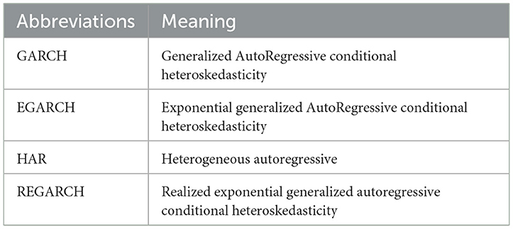
Table 1. Table of abbreviations.

2 Literature review

Accurately forecasting the crude oil futures volatility is important for market investors, risk managers and policy markers, since it has an important influence on investors' financial strategies and policymakers' decisions (Agnolucci, 2009; Wei et al., 2017; Wen et al., 2019; Lyu et al., 2021a,b; Huang et al., 2023). It has been well documented in the literature that financial Volatility exhibits complex characteristics, such as volatility clustering, leverage effects and mean-reverting properties, which poses great challenges in volatility measuring and forecasting. Traditionally, volatility estimator is derived from closing prices, and a variety of volatility models have been proposed to describe its dynamics in the last three decades. Since the seminal work by Engle (1982) and Bollerslev (1986), who propose the generalized autoregressive conditional heteroskedasticity (GARCH)-type models, numerous studies have been devoted to investigating the crude oil volatility modeling and forecasting by using GARCH-type models (see, e.g., Iglesias and Rivera-Alonso, 2022; Hong et al., 2022; Wang et al., 2021; Lin et al., 2020; Pan et al., 2017; Kang and Yoon, 2013). An alternative to the GARCH volatility model is the stochastic volatility (SV) models of Taylor (1986) and Heston (1993). Tsay (2005) presents a review of the two strands of the literature. Lyu et al. (2021a,b) analyse the time-varying effects of global economic uncertainty shocks on the volatilities of Brent and WTI crude oil prices through a time-varying parameter structural vector autoregressive model with stochastic volatility. Essentially, both the GARCH and SV models are return-based models, which are constructed based on daily closing prices, neglecting all intraday price movement, which reduces the predictive power of the models (Pu et al., 2016; Gong and Lin, 2018).

With the increasing availability of intraday high-frequency data, many authors have introduced the realized measures to measure the financial volatility (Andersen et al., 2001; Barndorff-Nielsen and Shephard, 2002, 2004; Kazemzadeh et al., 2023a,b, 2022). Corsi (2009) develop the HAR model based on realized volatility, which effectively captures the long-memory characteristics of volatility. Thanks to its ease of extensibility, the model has gained wide recognition and application. Wen et al. (2016) analyze the impact of stock market uncertainty on the volatility of the crude oil futures market by constructing an HAR model. Furthermore, Zhang et al. (2023) compare the performance of HAR models with different structural changes in forecasting the volatility of the crude oil futures market. Notably, the realized measure contains more information about the current level of volatility, which can provide more accurate volatility estimates (Andersen et al., 2001; Lyócsa et al., 2021). However, the realized measure based on intraday high-frequency data is sensitive to market microstructure noise, which leads to a biased volatility estimate.

As an alternative, the price range computed from the intraday high and low prices has been proposed to measure volatility. The idea of using price range in finance can be found in Mandelbrot (1971), who employs it to test the existence of long-term dependence in asset prices. The price range incorporates more (extreme-value) information on intra-period trajectory of the prices than the return-based volatility measure that only includes single measurement of the closing prices each period (Wu and Hou, 2020). Numerous studies have shown that the intraday price range is a more efficient measure of financial volatility relative to the commonly used return-based measure, such as the absolute (or squared) return or even the realized volatility from intraday returns. In fact, by employing the extreme-value theory and some well-known properties of range, Parkinson (1980) provide evidence of the superiority of using range as a volatility estimator. Alizadeh et al. (2002) show theoretically, numerically and empirically that range-based volatility estimator is not only highly efficient, but also approximately Gaussian and robust to microstructure noise. Brandt and Jones (2006) find that the range-based EGARCH model has better volatility forecast performance compared to the return-based EGARCH model. More recently, Degiannakis and Livada (2013) show that the price range volatility estimator is more accurate than the realized volatility estimator based on five, or less, equidistance points in time.

To explore the intraday (extreme-value) information for modeling volatility, motivated by the insights of the realized SV model (Shirota et al., 2014; Asai and McAleer, 2022), Hansen et al. (2012) develop a joint model of return and realized measure, namely the realized GARCH (RGARCH) model. The RGARCH model can capture the leverage effect of volatility, and is well suited for situations where volatility changes rapidly to a new level. Using the RGARCH model, Hansen et al. (2012) demonstrate that the inclusion of the realized measures can improve the model's ability to forecast volatility. Further, Hansen and Huang (2016) extend the RGARCH model to incorporate an additional leverage function to capture leverage effect more flexibly. The resulting model is referred to as the REGARCH model. Importantly, the R(E)GARCH model has a simple structure, which can be estimated and filtered easily. In addition, the model can automatically adjust the bias in the realized measures caused by non-trading hours and market microstructure noise. Subsequently, the R(E)GARCH model has attracted a great deal of attention in the literature. For example, Huang et al. (2017) and Tong and Huang (2021) apply the R(E)GARCH model to option pricing, and find that the R(E)GARCH model provide better option pricing performance than the traditional GARCH models. Chen and Watanabe (2019) and Chen et al. (2022) apply the R(E)GARCH model to risk measurement.

Despite the empirical success of the R(E)GARCH model, it does not take into account the presence of jumps in asset prices, which have been well recognized in the literature (see, e.g., Arouri et al., 2019; Pan et al., 2020; Qiao et al., 2020; Guo et al., 2023; Wu et al., 2024; Zhang et al., 2024). The huge changes (i.e., jumps) in asset prices usually cannot be explained by the current level of volatility. In recent years, numerous studies have shown that the occurrence of jumps is time-varying (see, e.g., Chernov et al., 2018; Zhou et al., 2019; Dutta et al., 2021). Most of these studies capture the risk of market crashes by assuming that the intensity of jumps is a function of the variance of asset returns. Although this modeling approach is intuitive and simple, it can not capture the jumps of asset price adequately.

Table 2 summarizes the relevant studies in the literature, while Table 3 provides an overview of the associated econometric models. Motivated by the above insights, in this paper we use price range as a proxy of realized measure, and propose the REGARCH-Jump model to modeling and forecasting the crude oil futures volatility. Notably, our proposed model can capture the extreme-value information as well as the dynamic jumps through assuming the jump intensity is governed by a autoregressive conditional jump intensity process. It is worth pointing out that although significant contributions have been made in the literature on crude oil futures volatility forecasting, few studies have taken into account both the extreme-value information and dynamic jumps in the crude oil futures prices for predicting the crude oil futures volatility.

Table 2

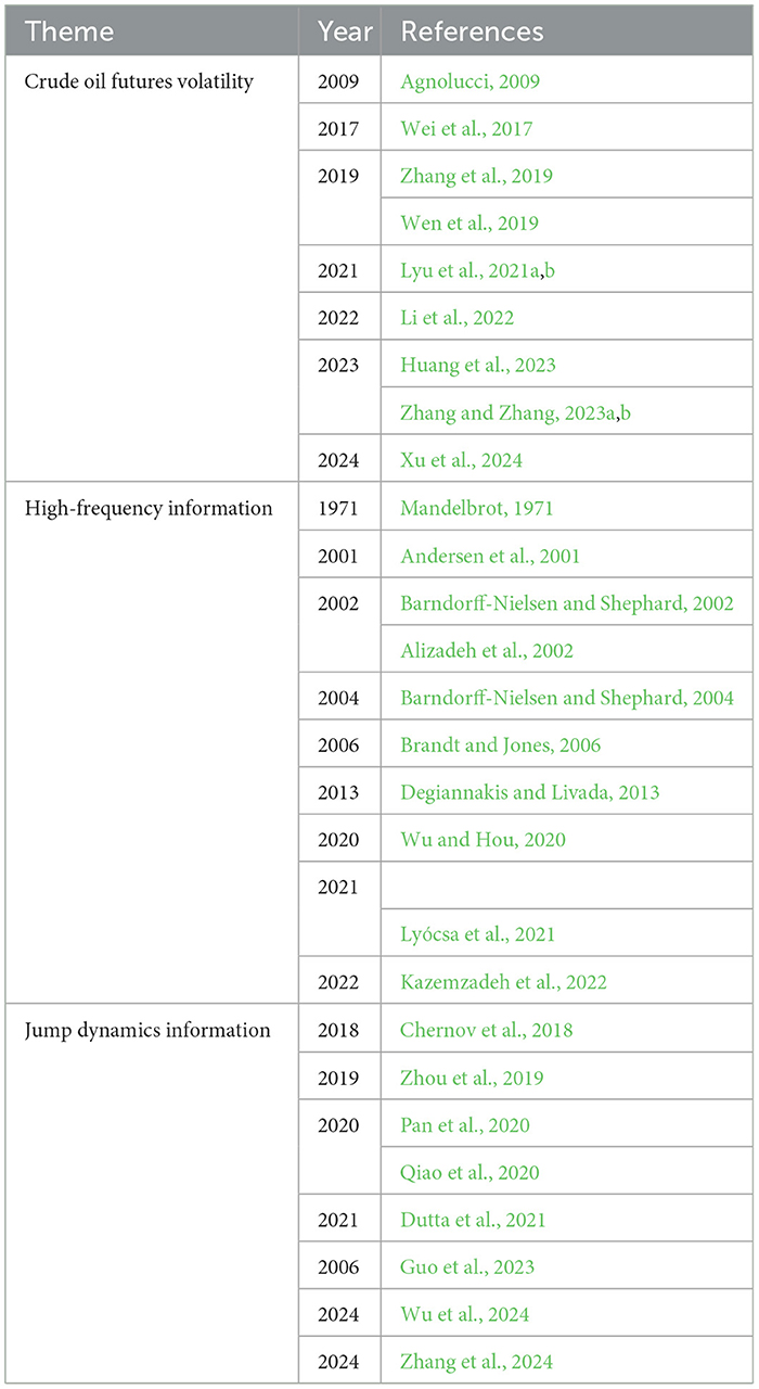
Table 2. Relevant literature review.

Table 3

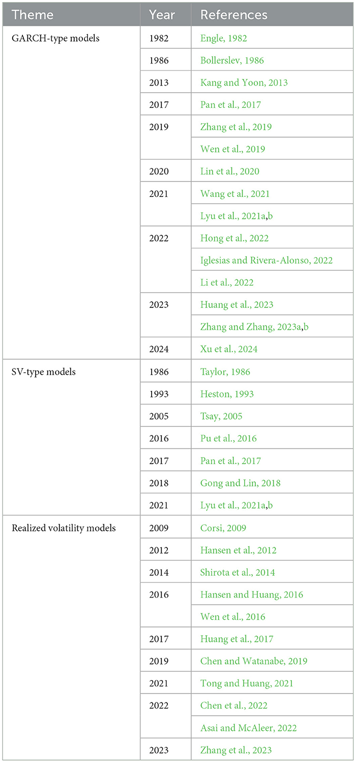
Table 3. Relevant models review.

3 The model

In this section, we first provide a brief review of the GARCH, the EGARCH, the HAR and the REGARCH models. Then we introduce the extension of the REGARCH model, namely the REGARCH-Jump model, which simultaneously accommodates the extreme-value information and time-varying jump intensity. Finally, we describe the maximum likelihood method for estimation of the parameters of the proposed model.

3.1 GARCH model

In financial econometric literature, the GARCH model proposed by Bollerslev (1986) is a popular approach for measuring and forecasting financial volatility. The GARCH model can be written as

$\begin{array}{ll}{r}_t=\mu +z_t& (1)\end{array}$

$\begin{array}{ll}{z}_t=\sqrt{h_t}{ϵ}_t,{ϵ}_t~i.i.d.N(0,1)& (2)\end{array}$

$\begin{array}{ll}{h}_t=\omega +\alpha z_{t-1}^2+\beta h_{t-1}& (3)\end{array}$

where r_t = log(P_t/P_t−1) is the log-return on day t, where P_t is the closing price on day t; μ is the conditional mean of r_t; h_t is the conditional variance of r_t; z_t is the return innovation, and ϵ_t is the standardized return innovation.

3.2 EGARCH model

The EGARCH model was proposed by Nelson (1991), which has the capacity to capture the leverage effect, which has been found to be important for volatility forecasting. The EGARCH model is given by

$\begin{array}{ll}{r}_t=\mu +z_t& (4)\end{array}$

$\begin{array}{ll}{z}_t=\sqrt{h_t}{ϵ}_t,{ϵ}_t~i.i.d.N(0,1)& (5)\end{array}$

$\begin{array}{ll}log(h_t)=\omega +\beta log(h_{t-1})+\gamma {ϵ}_{t-1}+\alpha (\left|{ϵ}_{t-1}\right|-E(\left|{ϵ}_{t-1}\right|))& (6)\end{array}$

where the coefficient γ captures the leverage effect when γ < 0.

3.3 HAR model

Based on the Heterogeneous Market Hypothesis, the HAR model proposed by Corsi (2009) aims to capture the volatility dynamics in financial markets, which can be written as

$\begin{array}{ll}{x}_{t+1}=c_t+{\beta }_d{x}_t+{\beta }_w{x}_t^w+{\beta }_m{x}_t^m+{\omega }_{t+1}& (7)\end{array}$

$\begin{array}{ll}{\omega }_t={\sigma }_d{ϵ}_t{ϵ}_t~i.i.d.N(0,1)& (8)\end{array}$

$\begin{array}{ll}{x}_t^w=\frac{x_t^d+x_{t-1}^d+\cdots +x_{t-4}^d}{5}& (9)\end{array}$

$\begin{array}{ll}{x}_t^m=\frac{x_t^d+x_{t-1}^d+\cdots +x_{t-21}^d}{22}& (10)\end{array}$

where x_t is the realized measure of volatility on day t; $x_t^w$ and $x_t^m$ represent the average realized volatility for the past weekly and monthly periods, respectively. (corresponding to lags of 5 days, and 22 days).

3.4 REGARCH model

Considering the fact that the RGARCH model cannot capture the leverage effect (asymmetric response of volatility to positive and negative shocks) adequately, Hansen and Huang (2016) extend the RGARCH to the REGARCH model, which can be written as

$\begin{array}{ll}{r}_t=\mu +z_t& (11)\end{array}$

$\begin{array}{ll}{z}_t=\sqrt{h_t}{ϵ}_t,{ϵ}_t~i.i.d.N(0,1)& (12)\end{array}$

$\begin{array}{ll}log(h_t)=\omega +\beta log(h_{t-1})+d({ϵ}_{t-1})+\alpha u_{t-1}& (13)\end{array}$

$\begin{array}{ll}log(x_t)=\xi +\phi log(h_t)+\upsilon ({ϵ}_t)+u_t,u_t~\text{i.i.d.}N(0,{\sigma }_u^2)& (14)\end{array}$

$\begin{array}{ll}d({ϵ}_t)=d_1{ϵ}_t+d_2({ϵ}_t^2-1)& (15)\end{array}$

$\begin{array}{ll}\upsilon ({ϵ}_t)={\upsilon }_1{ϵ}_t+{\upsilon }_2({ϵ}_t^2-1)& (16)\end{array}$

where u_t is the realized measure innovation, which is independent of the return innovation ϵ_t; d(ϵ_t) and υ(ϵ_t) are the leverage functions, which are used to capture the leverage effect, satisfying E_t−1[d(ϵ_t)] = E_t−1[v(ϵ_t)] = 0. If d₁ < 0, υ₁ < 0, it means that there exists leverage effect.

In the REGARCH model, Equations 11, 13 and 14 are referred to as the return equation, the variance (GARCH) equation and the measurement equation, respectively. The measurement equation relates the ex-post realized measure to the ex-ante conditional variance, with bias-correction coefficients ξ and φ used to correct the bias in the realized volatility measure caused by non-trading hours and market microstructure noise. Consistent with Takahashi et al. (2009), Koopman and Scharth (2012) and Wu et al. (2020), we assume that φ = 1 to facilitate model estimation and to improve out-of-sample performance.

3.5 REGARCH-jump model

The REGARCH model fall short in capturing the jumps (huge changes) in the asset prices. In light of this, this paper proposes the REGARCH-Jump model that extends the REGARCH model of Hansen and Huang (2016) to incorporate the dynamic jump intensity to model and forecast the volatility of crude oil futures markets. The specification of the REAGRCH-Jump model is as follows

$\begin{array}{ll}{r}_t=\mu +z_t+y_t& (17)\end{array}$

$\begin{array}{ll}{z}_t=\sqrt{h_{z,t}}{ϵ}_t,{ϵ}_t~i.i.d.N(0,1)& (18)\end{array}$

$\begin{array}{ll}{y}_t={\displaystyle \sum _{j=0}^{n_t}}{Y}_t^j,j=0,1,2,\dots ,n_t& (19)\end{array}$

$\begin{array}{ll}log(h_{z,t})=\omega +\beta log(h_{z,t-1})+d({ϵ}_{t-1})+\alpha u_{t-1}& (20)\end{array}$

$\begin{array}{ll}log(x_t)=\xi +\phi log(h_t)+\upsilon ({ϵ}_t)+u_t,u_t~i.i.d.N(0,{\sigma }_u^2)& (21)\end{array}$

where z_t and y_t denote the normal component and the jump component, respectively, which are assumed to be independent. The normal component z_t is assumed to be distributed as N(0, h_z,t), where h_z,t is the conditional variance of the normal component, which is governed by the REGARCH dynamic. The jump component y_t follows a compound Poisson process with jump intensity h_y,t and jump size $Y_t^j$, where $Y_t^j$ is independently drawn from a normal distribution with mean θ and variance δ², that is, $Y_t^j~i.i.d.N(\theta ,{\delta }^2)$. The mean and variance of the jump component, y_t, are given by θh_y,t and $({\theta }^2+{\delta }^2)h_{y,t}$, respectively. n_t is the number of jumps arriving between t − 1 and t, which follows a Poisson counting process with intensity h_y,t, that is, n_t ~ Poisson(h_y,t). The conditional probability of n_t can be written as

$\begin{array}{ll}\text{P}{\text{r}}_{t-1}(n_t=j)=\frac{exp(-h_{y,t})h_{y,t}^j}{j!},j=0,1,2,\dots & (22)\end{array}$

Therefore, the conditional expectation of the number of jumps arriving over the time interval (t − 1, t) equals the jump intensity, that is, E_t−1[n_t] = h_y,t. To describe the dynamics of jump intensity process h_y,t, we follow Maheu and McCurdy (2004) and assume that it follows the autoregressive conditional jump intensity model:

$\begin{array}{ll}{h}_{y,t}=\rho +\kappa h_{y,t-1}+\psi {\zeta }_{t-1}& (23)\end{array}$

where ρ > 0, κ > 0, ψ > 0; ζ_t−1 denotes the jump intensity residual, which can be written as

$\begin{array}{ll}\begin{array}{l}{\zeta }_{t-1}=E_{t-1}(n_{t-1})-h_{y,t-1}\\ ={\displaystyle \sum _{j=0}^{\infty }}j{Pr}_{t-1}(n_{t-1}=j)-h_{y,t-1}\end{array}& (24)\end{array}$

It is clear that E(ζ_t−1) = 0. Thus, κ describes the persistence of the jump intensity process. If h_y,t is stationary, we have 0 < κ < 1. Then the unconditional jump intensity is given by $E(h_{y,t})=\frac{\rho }{1-\kappa }$.

In the measurement Equation 21, h_t denotes the total unconditional variance of return, which can be written as

$\begin{array}{ll}{h}_t=h_{z,t}+({\theta }^2+{\delta }^2)h_{y,t}& (25)\end{array}$

It has been well documented in the literature that the use of intraday high and low prices leads to more accurate estimate of volatility than daily returns (Molnár, 2011; Chou and Liu, 2010). Therefore, in the paper we utilize the intraday price range calculated from the intraday high and low prices as a proxy for the realized measure in the HAR, REGARCH specifications, and their extensions. The intraday price range of Parkinson (1980) is defined as

$\begin{array}{ll}RN{G}_t=\frac{log(H_t)-log(L_t)}{\sqrt{4log(2)}}& (26)\end{array}$

where H_t and L_t are the high and low prices observed at day t, respectively. The intraday range given by Equation 26 is not only a highly efficient volatility proxy, capturing information regarding the entire intraday trajectory of the price, but also robust to microstructure noise (Alizadeh et al., 2002; Brandt and Jones, 2006). In this paper, we set $x_t=RN{G}_t^2$ the HAR, REGARCH specifications, and their extensions.

3.6 Maximum likelihood estimation

The proposed REGARCH-Jump model is intuitive and easy to implement. We can use the classical maximum likelihood method to estimate the parameters of the model. To be specific, the log-likelihood function of the REGARCH-Jump model can be written as

$\begin{array}{ll}\ell (r,x;\Theta )=\ell (r;\Theta )+\ell (x|r;\Theta )& (27)\end{array}$

$\begin{array}{ll}\ell (r;\Theta )\propto {\displaystyle \sum _{t=1}^T}ln(f_{t-1}(r_t))& (28)\end{array}$

$\begin{array}{ll}\ell (x|r;\Theta )\propto {\displaystyle \sum _{t=1}^T}ln(f_{t-1}(x_t|r_t))& (29)\end{array}$

where $\Theta ={(\mu ,\omega ,\alpha ,\beta ,d_1,d_2,\xi ,\phi ,{\sigma }_u,{\upsilon }_1,{\upsilon }_2,\rho ,\kappa ,\psi ,\theta ,\delta )}^{\prime }$ is the vector of model parameters, ℓ(r; Θ) and ℓ(x|r; Θ) are the partial log-likelihood functions for the returns and realized measure, respectively. f_t−1(r_t) and f_t−1(x_t|r_t) denote the conditional probability density functions of r_t and x_t, respectively, which can be written as

$\begin{array}{ll}{f}_{t-1}(r_t)={\displaystyle \sum _{j=0}^{\infty }}{f}_{t-1}(r_t\mid n_t=j)\text{P}{\text{r}}_{t-1}(n_t=j)& (30)\end{array}$

$\begin{array}{ll}{f}_{t-1}(x_t\mid r_t)=\frac{1}{\sqrt{2\pi {\sigma }_u^2}}exp\left(-\frac{{(log(x_t)-\xi -\phi log(h_t)-v({ϵ}_t))}^2}{2{\sigma }_u^2}\right)& (31)\end{array}$

where Pr_t−1(n_t = j) is the conditional probability of the number of jumps, which is given in Equation 22. It should be noted that the summation in Equation 30 must be truncated when implementing the maximum likelihood estimation. We truncate the summation at 50 jumps per day. In fact, since the tail probability of Poisson distribution at n_t ≥ 50 is sufficiently small and negligible, summing to n_t = 50 can ensures the accuracy of the estimation process. f_t−1(r_t ∣ n_t = j) in Equation 30 can be written as

$\begin{array}{ll}{f}_{t-1}(r_t\mid n_t=j)=\frac{1}{\sqrt{2\pi (h_{z,t}+j{\delta }^2)}}exp\left(-\frac{{(r_t-\mu -j\theta )}^2}{2(h_{z,t}+j{\delta }^2)}\right)& (32)\end{array}$

In order to calculate the likelihoods (Equations 30–32), it is necessary to determine the normal innovation z_t and the number of jumps n_t, and further filter the conditional variance h_z,t+1 and the conditional jump intensity h_y,t+1. This process can be easily implemented by using analytic filtering. Applying Bayes' rule, the filtering density is given by

$\begin{array}{ll}\begin{array}{l}{Pr}_t(n_t=j)\equiv {Pr}_{t-1}(n_t=j\mid r_t)\\ =\frac{f_{t-1}(r_t\mid n_t=j){Pr}_{t-1}(n_t=j)}{f_{t-1}(r_t)}\end{array}& (33)\end{array}$

where the expressions on the right-hand side of the Equation 33 are given by Equations 22, 30 and 32. Pr_t(n_t = j) represents the ex-post inference on n_t, or the probability that j jumps have arrived between time t − 1 and t conditional on the information available at time t. The filtered number of jumps is then given by

$\begin{array}{ll}{ñ}_t=E_t(n_t)={\displaystyle \sum _{j=0}^{\infty }}j{Pr}_t(n_t=j)& (34)\end{array}$

The actual number of jumps, n_t, can be larger than one but is restricted to be less than fifty as mentioned above. According to Christoffersen et al. (2012), the filtering of the normal innovation z_t can be written as

$\begin{array}{ll}{\tilde{z}}_t=E_t(z_t)={\displaystyle \sum _{j=0}^{\infty }}\frac{{\tilde{h}}_{z,t}}{{\tilde{h}}_{z,t}+j{\delta }^2}(r_t-\mu -j\theta ){Pr}_t(n_t=j)& (35)\end{array}$

Once ñ_t and ${\tilde{z}}_t$ are known, we can infer the filtered ${\tilde{h}}_{z,t+1}$ and ${\tilde{h}}_{y,t+1}$ easily through Equations 20 and 23.

Finally, the parameters of the REGARCH-Jump model can be estimated via maximum likelihood method by solving

$\begin{array}{ll}\widehat{\Theta }=arg{\displaystyle \underset{\Theta }{max}}\ell (r,x;\Theta )& (36)\end{array}$

4 Volatility forecast evaluation

4.1 Loss function

The loss function is commonly used to evaluate the forecasting accuracy of the competing models. In the paper, we employ four popular loss functions, including the mean absolute error (MAE), mean absolute percentage error (MAPE), mean squared error (MSE) and Quasi-likelihood (QLIKE). The four evaluation criteria are defined as

$\begin{array}{ll}MAE=\frac{1}{T}{\displaystyle \sum _{t=1}^T}|h_{t+1}-{ĥ}_{t+1}(m)|& (37)\end{array}$

$\begin{array}{ll}MAPE=\frac{1}{T}{\displaystyle \sum _{t=1}^T}\left|\frac{h_{t+1}-{ĥ}_{t+1}(m)}{h_{t+1}}\right|& (38)\end{array}$

$\begin{array}{ll}MSE=\frac{1}{T}{\displaystyle \sum _{t=1}^T}(h_{t+1}-{ĥ}_{t+1}(m){)}^2& (39)\end{array}$

$\begin{array}{ll}QLIKE=\frac{1}{T}{\displaystyle \sum _{t=1}^T}(\frac{h_{t+1}}{{ĥ}_{t+1}(m)}-log(\frac{h_{t+1}}{{ĥ}_{t+1}(m)})-1)& (40)\end{array}$

where T is the number of out-of-sample forecasts, h_t+1 and ĥ_t+1(m) denote the measured (true) volatility and forecasted volatility, respectively, and m stands for the GARCH, EGARCH, HAR, REGARCH or REGARCH-Jump models. It is worth noting that MSE and QLIKE are robust loss functions, which could provide a consistent ranking of the volatility models with a conditionally unbiased volatility proxy (Patton, 2011).

Since the true volatility is unobservable, the evaluation and comparison of volatility forecasting models requires the proxy of true volatility. In the paper, we employ the scaled realized volatility (RV) as a proxy of the true volatility. The scaled RV is defined as $R{V}_t^{scale}=c\times R{V}_t$, where RV_t is computed based 5-min intraday returns on day t and $c=\sum _{t=1}^T{r}_t^2/\sum _{t=1}^{T}R{V}_t$. This adjustment is used to account for the non-trading hours.

4.2 MCS test

For robustness, we adopt the model confidence set (MCS) test proposed by Hansen et al. (2011) to examine whether the difference in forecasting performance between the competing models is statistically significant. The MCS method tests a given set of competing models and identifies a set of optimal predictive models or MCS with a certain level of confidence. Specifically, the MCS test relies on an equivalence test δ_{$\mathcal{M}$} and an elimination rule e_{$\mathcal{M}$}. Let $\mathcal{M}$⁰ be the initial set of all competing models. Set $\mathcal{M}$ = $\mathcal{M}$⁰, and use the equivalence test δ_{$\mathcal{M}$} to test the null hypothesis that the competing models have the same expected loss (equal forecasting performance), i.e.,

$\begin{array}{ll}{H}_{0,\mathcal{M}}:E\left[d_{uv,t}\right]=0,\forall u,v\in \mathcal{M}& (41)\end{array}$

where d_uv,t = Loss_t(u)−Loss_t(v) is the loss difference between the models u and v. Hansen et al. (2011) propose the following statistics to test the null hypothesis H_{0,$\mathcal{M}$}:

$\begin{array}{ll}{T}_{\mathcal{M}}={\displaystyle \underset{u,v\in \mathcal{M}}{max}}\left|t_{uv}\right|,t_{uv}=\frac{{\bar{d}}_{uv}}{\sqrt{\widehat{\text{var}}({\bar{d}}_{uv})}}& (42)\end{array}$

where ${\bar{d}}_{uv}$ is the average loss difference, and $\widehat{\text{var}}({\bar{d}}_{uv})$ is the bootstrapped estimate of the variance of ${\bar{d}}_{uv}$, i.e., $\text{var}({\bar{d}}_{uv})$. For a given significance level α, if the null hypothesis H_{0,$\mathcal{M}$} is accepted, define ${\mathcal{M}}_{1-\alpha }^{*}=\mathcal{M}$. Otherwise, we use the elimination rule $e_{\mathcal{M}}=arg{max}_{u\in \mathcal{M}}{sup}_{v\in \mathcal{M}}{t}_{uv}$ to exclude the model that has poor forecasting performance. This process is repeated until no model can be excluded. Finally, the set of surviving models ${\mathcal{M}}_{1-\alpha }^{*}=\mathcal{M}$ is referred to as the MCS, i.e. the set of optimal predictive models at a given confidence level of 1 − α.

Since the asymptotic distribution of the test statistics T_{$\mathcal{M}$} is non-standard, this paper uses a block bootstrap of 10⁵ replications for approximate calculation. In addition, we set the significance level as α = 10%.

5 Empirical application

5.1 Data and descriptive statistics

For our empirical analysis, we use data on the daily open, high, low and close prices for the Brent crude oil futures. We focus on Brent crude oil futures market due to the fact that Brent crude oil is currently considered to be the global oil pricing benchmark (Dowling et al., 2016; Zavadska et al., 2020). We employ the squared price range ($RN{G}_t^2$) as the realized volatility measure (i.e., x_t). The data is obtained from Wind Database of China, and the sample period is from January 4, 2005 to February 28, 2023.

Table 4 presents the descriptive statistics of the daily returns and price ranges of Brent crude oil futures. As can be seen from the table, the return distribution for the Brent crude oil futures is negatively skewed and leptokurtic, while the price range distribution is positively skewed and leptokurtic. The Jarque-Bera statistics indicate that both the return and price range distributions are non-Gaussian. The Ljung-Box Q-statistic for autocorrelation up to 20 lags shows that the price range series is highly autocorrelated, suggesting high persistence of Brent crude oil futures volatility.

Table 4

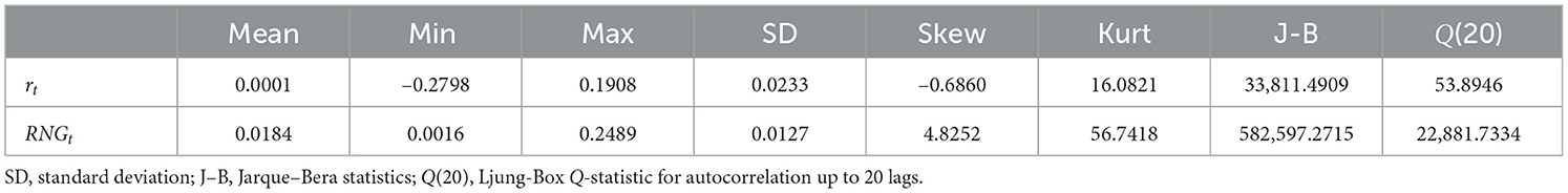
Table 4. Descriptive statistics of Brent crude oil futures.

Figure 1 presents the time series plots of the daily Brent crude oil futures returns and price ranges. It can be seen from the figure that the well-known behavior of volatility clustering is apparent. In addition, the Brent crude oil futures experience large fluctuations (jumps) during the periods of 2008–2009 global financial crisis (GFC), 2020 COVID-19 pandemic and 2022 Russo-Ukrainian conflict.

Figure 1

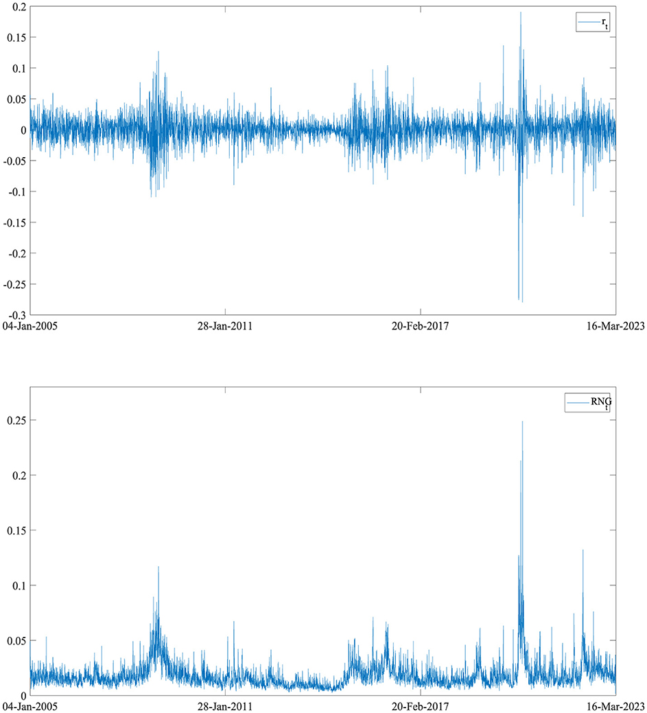
Figure 1. Time series plots of the daily Brent crude oil futures returns and price ranges.

5.2 In-sample parameter estimation

In this subsection, we estimate the five competitor models (GARCH, EGARCH, HAR, REGARCH and REGARCH-Jump) using the maximum likelihood method based on the in-sample data covering the period from January 4, 2005 to December 31, 2020. Table 5 reports the maximum likelihood estimates for the five models. As can be seen from the table, the daily coefficient of x_t in the HAR model is significantly positive, while the weekly coefficient is significantly negative. This indicates that daily information positively affects crude oil futures volatility, whereas weekly information has a negative impact. Additionally, the estimates of volatility persistence in the GARCH, EGARCH, REGARCH and REGARCH-Jump models are larger than 0.98, suggesting the stylized fact of high volatility persistence. Regarding the leverage parameters, γ, d₁, d₂, υ₁ and υ₂, they are all significantly different from zero. In particular, γ, d₁ and υ₁ are all negative, suggesting the presence of the leverage effect in the Brent crude oil futures market.

Table 5

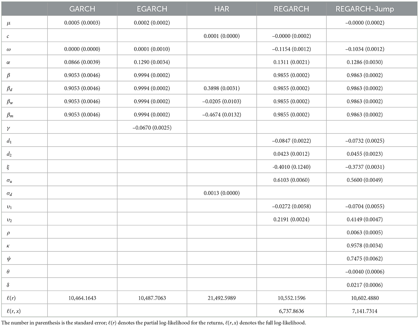
Table 5. Parameter estimation results for the Brent crude oil futures.

Moreover, the jump intensity parameters (ρ, κ, ψ) are all positive and statistically significant, suggesting the presence of time-varying jump intensity and that the REGARCH-jump model is correctly specified. In particular, the parameter κ is estimated to be 0.9578, which provides evidence of high persistence of the conditional jump intensity process. The estimated mean jump size θ in the REGARCH-Jump model is significantly negative, while the estimated jump volatility δ is significantly positive. The unconditional mean of dynamic jump intensity is $E(h_{y,t})=\frac{\rho }{1-\kappa }=0.1493$, implying that jumps arrive at a frequency of 37.6 jumps per year. In addition, the contribution of return jumps to the total return variance is $\frac{({\theta }^2+{\delta }^2)h_{y,t}}{({\theta }^2+{\delta }^2)h_{y,t}+h_{z,t}}=12.73\%$, which is close to the results reported in Christoffersen et al. (2012) (12%~15%), Andersen et al. (2007) (14.6%) and Pan et al. (2020) (11%), suggesting that our estimation results of jump intensity is reasonable.

Finally, we can observe that the REGARCH-Jump model improves the empirical return fit relative to all other models (GARCH, EGARCH and REGARCH) in terms of the partial log-likelihood for the returns ℓ(r) and the full log-likelihood ℓ(r, x).

Figure 2 presents the time series plots of the jump intensity and the number of jumps. It is clear that the jumps have a time-varying feature, and the number of jumps related to market uncertainty events have increased during the periods of 2008–2009 global financial crisis, 2015 global oil price decline and 2020 COVID-19 pandemic. Note also that, the number of jumps in most cases is less than one jump per day.

Figure 2

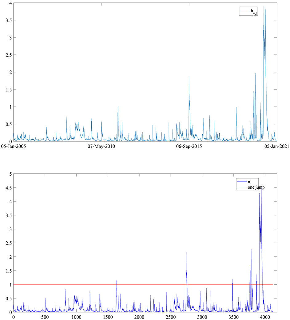
Figure 2. Time series plots of the jump intensify h_y,t and the number of jumps n_t for the Brent crude oil futures.

5.3 Out-of-sample forecast results

In the in-sample analysis, we document that the jump intensity and the number of jumps has time-varying characteristic. Moreover, we show that incorporating the extreme-value information and jump dynamics into the REGARCH model could improve the model's ability to fit the Brent crude oil futures returns. In this subsection, we investigate the importance of accounting for the extreme-value information and jump dynamics for forecasting the crude oil futures volatility relying on our proposed REGARCH-Jump model. Importantly, we compare the out-of-sample forecasting performance of the REGARCH-Jump model with that of the GARCH, EGARCH, HAR and REGARCH models.

The out-of-sample forecast exercise is performed relying on a rolling window scheme. The out-of-sample period is from January 4, 2021 to February 28, 2023. Figure 3 presents the out-of-sample volatility forecasts for the competing models. Table 6 reports the out-of-sample forecast evaluation results based on the four loss functions. As can be seen from the table, the REGARCH model offers smaller loss values (MAE, MAPE, MSE, QLIKE) than the GARCH and EGARCH models. In particular, the REGARCH-Jump model yields the smallest loss values in all cases. Our findings indicate that incorporating the extreme-value information and jump dynamics into volatility model is important for improving the out-of-sample volatility forecasts.

Figure 3

Figure 3. Out-of-sample volatility forecasts.

Table 6

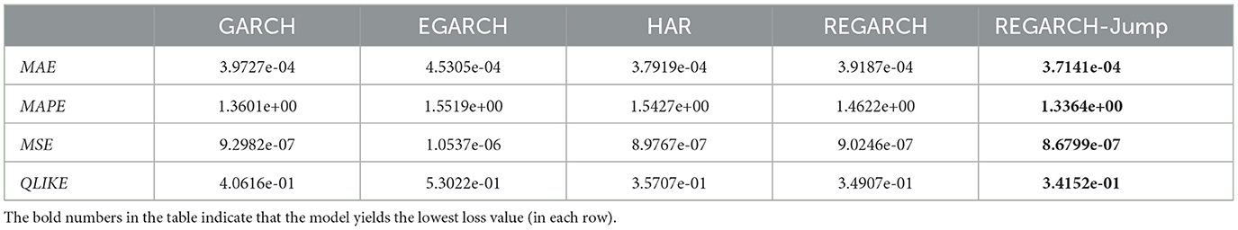
Table 6. Out-of-sample forecast evaluation results.

Further, Table 7 presents the MCS test results for the out-of-sample forecasts of competing models. It is clear that the REGARCH-Jump model is always included in the MCS, and always has the highest MCS p-value (p = 1), confirming the superior performance of the REGARCH-Jump model over all other models in forecasting the crude oil futures volatility.

Table 7

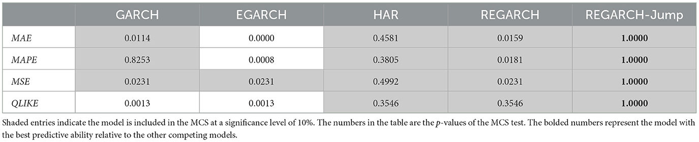
Table 7. MCS test results.

5.4 Robustness check

For robustness, we perform the out-of-sample forecast exercise for different out-of-sample windows. To be specific, we consider two alternative out-of-sample windows: 200 and 400. The out-of-sample forecast evaluation results for the alternative out-of-sample windows are reported in Table 8.

Table 8

Table 8. Out-of-sample forecast evaluation results for alternative out-of-sample windows.

In line with the results reported in Tables 6, 7, the REGARCH-Jump model that accounts for the extreme-value information and jump dynamics yields the most accurate volatility forecasts, dominating all other models. This result confirms that the superior performance of the REGARCH-Jump model in forecasting the crude oil futures volatility is robust to alternative out-of-sample forecast windows.

5.5 Economic value analysis

To illustrate the economic value of the improved volatility forecasts from the REGARCH-Jump model, we perform a VaR analysis in this subsection. Accurate measurement of financial market risk is of great significance to the investors, policy makers and regulators who are trying to manage the risk of portfolio as well as to maintain the functioning and the stability of financial markets. The standard tool for measuring market risk is VaR, which is intuitive, simple and easy to compute. It is used by financial institutions and financial regulators worldwide for market risk mointoring and management.

5.5.1 VaR forecast

The one-day-ahead forecast of VaR for a given probability (significance level) α satisfies:

$\begin{array}{ll}\text{P}{\text{r}}_{t-1}(r_t<Va{R}_t(\alpha ))=\alpha & (43)\end{array}$

According to the definition of VaR in Equation 39, the VaR under the REGARCH-Jump model can be formulated as

$\begin{array}{ll}Va{R}_t(\alpha )=\mu +{\widetilde{ϵ}}_{\alpha }\sqrt{h_{z,t}+({\theta }^2+{\delta }^2)h_{y,t}}& (44)\end{array}$

where $\widetilde{{ϵ}_{\alpha }}$ can be written as follows (Chiu et al., 2006):

$\begin{array}{ll}{\widetilde{ϵ}}_{\alpha }={ϵ}_{\alpha }+\frac{1}{6}({ϵ}_{\alpha }-1)\times Sk(r_t)& (45)\end{array}$

$\begin{array}{ll}Sk(r_t)=\frac{h_{y,t}({\theta }^3+3\theta {\delta }^2)}{(h_{z,t}+h_{y,t}{\theta }^2+h_{y,t}{\delta }^2{)}^{3/2}}& (46)\end{array}$

where ϵ_α is the left quantile at level α for standard normal distribution, and Sk(r_t) is the conditional skewness of returns.

5.5.2 Backtesting

To examine the accuracy of VaR forecast, we perform the backtesting relying on the failure rate test, the likelihood ratio test of unconsitional coverage (Kupiec, 1995) and the likelihood ratio test of consitional coverage (Christoffersen, 1998).

The likelihood ratio test statistic of unconsitional coverage can be written as

$\begin{array}{ll}L{R}_{uc}=-2ln[{\alpha }^{T_1}{(1-\alpha )}^{T_1-T_0}F{R}^{-T_0}{(1-FR)}^{T_1-T_0}]~{\chi }^2(1)& (47)\end{array}$

where FR is failure rate, that is, FR = T₀/T₁, T₀ is the number of times the VaR is violated, T₁ is the total number of VaR forecasts.

The likelihood ratio test statistic of unconsitional coverage (LR_uc) can not examine the independence of VaR exceptions. In light of this, Christoffersen (1998) propose the conditional coverage test that can examine the independence of VaR exceptions, which can be written as

$\begin{array}{ll}L{R}_{cc}=L{R}_{uc}+L{R}_{ind}~{\chi }^2(2)& (48)\end{array}$

where

$\begin{array}{ll}L{R}_{ind}=-2ln\left[\frac{{(1-F{R}_2)}^{T_{00}+T_{10}}F{R}_2^{T_{00}+T_{11}}}{{(1-F{R}_{01})}^{T_{00}}F{R}_{01}^{T_{10}}F{R}_{11}^{T_{11}}}\right]~{\chi }^2(1)& (49)\end{array}$

and T_ij is the number of observations with value i followed by j, $F{R}_{01}=\frac{T_{01}}{T_{00}+T_{01}}$, $F{R}_{11}=\frac{T_{11}}{T_{10}+T_{11}}$, $F{R}_2=\frac{T_{01}+T_{11}}{T_{00}+T_{01}+T_{10}+T_{11}}$. It is clear that the conditional coverage test LR_cc builds on the LR_uc and LR_ind tests.

Figure 4 presents the VaR forecasts for the competing models. Table 9 reports the results of VaR backtesting including the failure rates (FR) test, the likelihood ratio test of unconsitional coverage (LR_uc) and the likelihood ratio test of consitional coverage (LR_cc) for the five competing models. As can be seen from Table 9, all models have passed the likelihood ratio test at the 10% and 5% significance levels, indicating that they all perform well in measuring the crude oil futures market risk in the cases. Importantly, it is interesting to note that the FR of the VaR forecasts for the REGARCH-Jump model are closer to the corresponding theoretical values (α) under the 95% and 90% confidence levels than the other models.

Figure 4

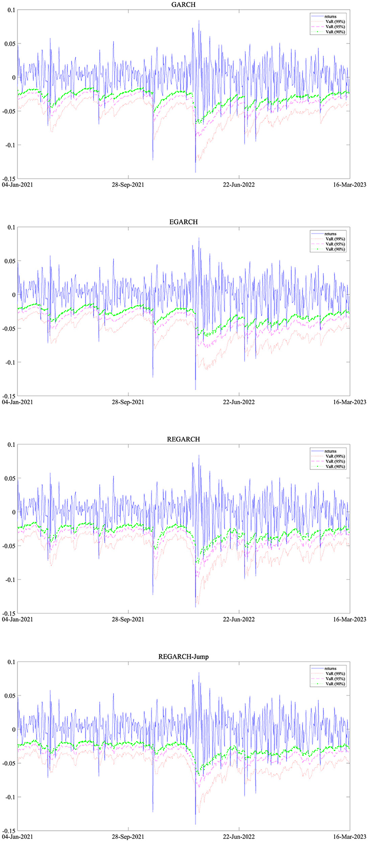
Figure 4. VaR forecasts.

Table 9

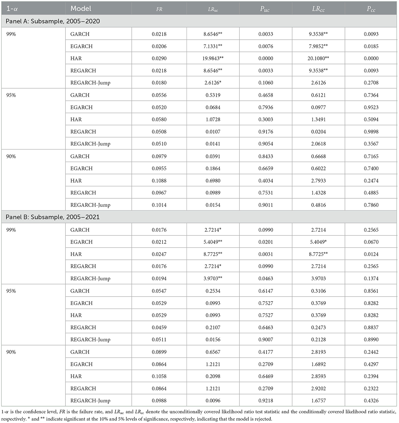
Table 9. Backtesting analysis of VaR forecasts.

Regarding the confidence level of 99%, the FR of VaR forecasts of the EGARCH model significantly deviates from the theoretical value (α = 0.01), and all of the models can not forecast VaR accurately in terms of the unconditionally covered likelihood ratio test. However, in terms of the conditionally covered likelihood ratio test, all the models except for the EGARCH model performs well.

Finally, we can observe that, based on the 95% and 90% confidence levels, the VaR forecasts obtained by the GARCH, EGARCH, HAR and REGARCH models are more conservative than that obtained by the REGARCH-Jump model, which may underestimate the risk. In summary, our results provide support for combining the extreme-value information and dynamic jumps for improving the accuracy of VaR forecasts. Note also that there is still room to improve the accuracy of VaR forecasts in extreme risk scenarios.

6 Conclusion

In this paper, we propose the REGARCH-Jump model, which incorporates the extreme-value information and jump dynamics, to model and forecast the crude oil futures volatility. An empirical analysis based on the daily Brent crude oil futures prices data shows the presence of time-varying jump intensity with high persistence. In addition, we observe that the REGARCH-Jump model outperforms the GARCH, EGARCH, HAR and REGARCH models in terms of both empirical return fit and out-of-sample volatility forecast. Moreover, we confirm that the superior forecasting performance of the REGARCH-Jump model is robust to alternative out-of-sample forecast windows. Finally, a VaR analysis is conducted to demonstrate the economic value of the improved volatility forecasts from the REGARCH-Jump model. We confirm that the REGARCH-Jump model can produce reasonable VaR forecasts. In summary, our findings highlight the importance of accommodating the extreme-value information as well as the jump dynamics in forecasting the volatility of the crude oil futures market.

Our work offers theoretical and methodological insights into modeling and forecasting the crude oil futures volatility, with great significance related to both academic researchers and practitioners. Further extensions and applications of the proposed model are encouraged. For example, incorporating intraday high-frequency data into the realized volatility measure presents a promising area for future research. In addition, future studies could involve applying the model to derivative pricing and asset allocation.

Data availability statement

The original contributions presented in the study are included in the article/supplementary material, further inquiries can be directed to the corresponding author.

Author contributions

WS: Methodology, Software, Supervision, Writing – review & editing. HL: Conceptualization, Data curation, Formal analysis, Writing – original draft.

Funding

The author(s) declare financial support was received for the research, authorship, and/or publication of this article. This research was supported by the National Natural Science Foundation of China [71971001]; Natural Science Foundation of Anhui Province [2208085Y21]; Academic Funding Project for Top Academic Talents in Anhui Universities [gxbjZD2022019]; Outstanding Youth Research Project for Anhui Universities [2022AH020047]; Innovative Research Project for Graduates of Anhui University of Finance and Economics under Grant No. ACYC2023137.

Conflict of interest

The authors declare that the research was conducted in the absence of any commercial or financial relationships that could be construed as a potential conflict of interest.

Generative AI statement

The author(s) declare that no Gen AI was used in the creation of this manuscript.

Publisher's note

All claims expressed in this article are solely those of the authors and do not necessarily represent those of their affiliated organizations, or those of the publisher, the editors and the reviewers. Any product that may be evaluated in this article, or claim that may be made by its manufacturer, is not guaranteed or endorsed by the publisher.

References

Agnolucci, P. (2009). Volatility in crude oil futures: a comparison of the predictive ability of GARCH and implied volatility models. Energy Econ. 31, 316–321. doi: 10.1016/j.eneco.2008.11.001

Crossref Full Text | Google Scholar

Alizadeh, S., Brandt, M. W., and Diebold, F. X. (2002). Range-based estimation of stochastic volatility models. J. Finance 57, 1047–1091. doi: 10.1111/1540-6261.00454

Crossref Full Text | Google Scholar

Andersen, T. G., Bollerslev, T., and Diebold, F. X. (2007). Roughing it up: including jump components in the measurement, modeling, and forecasting of return volatility. Rev. Econ. Stat. 89, 701–720. doi: 10.1162/rest.89.4.701

Crossref Full Text | Google Scholar

Andersen, T. G., Bollerslev, T., Diebold, F. X., and Ebens, H. (2001). The distribution of realized stock return volatility. J. Financ. Econ. 61, 43–76. doi: 10.1016/S0304-405X(01)00055-1

Crossref Full Text | Google Scholar

Arouri, M., M'saddek, O., and Pukthuanthong, K. (2019). Jump risk premia across major international equity markets. J. Empir. Finance 52, 1–21. doi: 10.1016/j.jempfin.2019.02.004

Crossref Full Text | Google Scholar

Asai, M., and McAleer, M. (2022). Bayesian analysis of realized matrix-exponential GARCH models. Comput. Econ. 59, 103–123. doi: 10.1007/s10614-020-10074-6

Crossref Full Text | Google Scholar

Barndorff-Nielsen, O. E., and Shephard, N. (2002). Econometric analysis of realised volatility and its use in estimating stochastic volatility models. J. R. Stat. Soc. Ser. B: Stat. Methodol. 64, 253–280. doi: 10.1111/1467-9868.00336

Crossref Full Text | Google Scholar

Barndorff-Nielsen, O. E., and Shephard, N. (2004). Power and bipower variation with stochastic volatility and jumps. J. Financ. Econom. 2, 1–37. doi: 10.1093/jjfinec/nbh001

PubMed Abstract | Crossref Full Text | Google Scholar

Bollerslev, T. (1986). Generalized autoregressive conditional heteroskedasticity. J. Econom. 31, 307–327. doi: 10.1016/0304-4076(86)90063-1

Crossref Full Text | Google Scholar

Brandt, M. W., and Jones, C. S. (2006). Volatility forecasting with range-based EGARCH models. J. Bus. Econ. Stat. 24, 470–486. doi: 10.1198/073500106000000206

PubMed Abstract | Crossref Full Text | Google Scholar

Chen, C. W. S., Lin, E. M. H., and Huang, T. F. J. (2022). Bayesian quantile forecasting via the realized hysteretic GARCH model. J. Forecast. 41, 1317–1337. doi: 10.1002/for.2876

Crossref Full Text | Google Scholar

Chen, C. W. S., and Watanabe, T. (2019). Bayesian modeling and forecasting of value-at-risk via threshold realized volatility. Appl. Stoch. Models Bus. Ind. 35, 747–765. doi: 10.1002/asmb.2395

Crossref Full Text | Google Scholar

Chernov, M., Graveline, J., and Zviadadze, I. (2018). Crash risk in currency returns. J. Financ. Quant. Anal. 53, 137–170. doi: 10.1017/S0022109017000801

PubMed Abstract | Crossref Full Text | Google Scholar

Chiu, C. L., Chiang, S. M., Hung, J. C., and Chen, Y.-L. (2006). Clearing margin system in the futures markets? Applying the value-at-risk model to Taiwanese data. Phys. A Stat. Mech. Appl. 367, 353–374. doi: 10.1016/j.physa.2005.12.034

Crossref Full Text | Google Scholar

Chou, R. Y., and Liu, N. (2010). The economic value of volatility timing using a range-based volatility model. J. Econ. Dyn. Control 34, 2288–2301. doi: 10.1016/j.jedc.2010.05.010

Crossref Full Text | Google Scholar

Christoffersen, P., Jacobs, K., and Ornthanalai, C. (2012). Dynamic jump intensities and risk premiums: evidence from S&P500 returns and options. J. Financ. Econ. 106, 447–472. doi: 10.1016/j.jfineco.2012.05.017

Crossref Full Text | Google Scholar

Christoffersen, P. F. (1998). Evaluating interval forecasts. Int. Econ. Rev. 39, 841–862. doi: 10.2307/2527341

Crossref Full Text | Google Scholar

Corsi, F. (2009). A simple approximate long-memory model of realized volatility. J. Financ. Econom. 7, 174–196. doi: 10.1093/jjfinec/nbp001

PubMed Abstract | Crossref Full Text | Google Scholar

Degiannakis, S., and Livada, A. (2013). Realized volatility or price range: evidence from a discrete simulation of the continuous time diffusion process. Econ. Model. 30, 212–216. doi: 10.1016/j.econmod.2012.09.027

Crossref Full Text | Google Scholar

Dowling, M., Cummins, M., and Lucey, B. M. (2016). Psychological barriers in oil futures markets. Energy Econ. 53, 293–304. doi: 10.1016/j.eneco.2014.03.022

Crossref Full Text | Google Scholar

Dutta, A., Bouri, E., and Roubaud, D. (2021). Modelling the volatility of crude oil returns: jumps and volatility forecasts. Int. J. Finance Econ. 26, 889–897. doi: 10.1002/ijfe.1826

Crossref Full Text | Google Scholar

Engle, R. F. (1982). Autoregressive conditional heteroscedasticity with estimates of the variance of United Kingdom inflation. Econometrica 50, 987–1007. doi: 10.2307/1912773

Crossref Full Text | Google Scholar

Gong, X., and Lin, B. (2018). Structural changes and out-of-sample prediction of realized range-based variance in the stock market. Phys. A Stat. Mech. Appl. 494, 27–39. doi: 10.1016/j.physa.2017.12.004

Crossref Full Text | Google Scholar

Guo, Y., Li, P., and Wu, H. (2023). Jumps in the Chinese crude oil futures volatility forecasting: new evidence. Energy Econ. 126:106955. doi: 10.1016/j.eneco.2023.106955

PubMed Abstract | Crossref Full Text | Google Scholar

Hansen, P. R., and Huang, Z. (2016). Exponential GARCH modeling with realized measures of volatility. J. Bus. Econ. Stat. 34, 269–287. doi: 10.1080/07350015.2015.1038543

Crossref Full Text | Google Scholar

Hansen, P. R., Huang, Z., and Shek, H. H. (2012). Realized GARCH: a joint model for returns and realized measures of volatility. J. Appl. Econ. 27, 877–906. doi: 10.1002/jae.1234

Crossref Full Text | Google Scholar

Hansen, P. R., Lunde, A., and Nason, J. M. (2011). The model confidence set. Econometrica 79, 453–497. doi: 10.3982/ECTA5771

Crossref Full Text | Google Scholar

Heston, S. L. (1993). A closed-form solution for options with stochastic volatility with applications to bond and currency options. Rev. Financ. Stud. 6, 327–343. doi: 10.1093/rfs/6.2.327

Crossref Full Text | Google Scholar

Hong, Y., Wang, L., Liang, C., and Umar, M. (2022). Impact of financial instability on international crude oil volatility: new sight from a regime-switching framework. Resour. Policy 77:102667. doi: 10.1016/j.resourpol.2022.102667

Crossref Full Text | Google Scholar

Huang, Y., Xu, W., Huang, D., and Zhao, C. (2023). Chinese crude oil futures volatility and sustainability: a uncertainty indices perspective. Resour. Policy 80:103227. doi: 10.1016/j.resourpol.2022.103227

Crossref Full Text | Google Scholar

Huang, Z., Wang, T. Y., and Hansen, P. R. (2017). Option pricing with the realized GARCH model: an analytical approximation approach. J. Futures Mark. 37, 328–358. doi: 10.1002/fut.21821

Crossref Full Text | Google Scholar

Iglesias, E. M., and Rivera-Alonso, D. (2022). Brent and WTI oil prices volatility during major crises and COVID-19. J. Petrol. Sci. Eng. 211:110182. doi: 10.1016/j.petrol.2022.110182

Crossref Full Text | Google Scholar

Kang, S. H., and Yoon, S. M. (2013). Modeling and forecasting the volatility of petroleum futures prices. Energy Econ. 36, 354–362. doi: 10.1016/j.eneco.2012.09.010

Crossref Full Text | Google Scholar

Kazemzadeh, E., Ahmadi Shadmehri, M. T., Ebrahimi Salari, T., Salehnia, N., and Pooya, A. (2022). Oil price shocks on shale oil supply and energy security: a case study of the United States. Int. J. Dev. Issues 21, 249–270. doi: 10.1108/IJDI-12-2021-0264

Crossref Full Text | Google Scholar

Kazemzadeh, E., Ahmadi Shadmehri, M. T., Ebrahimi Salari, T., Salehnia, N., and Pooya, A. (2023a). Modeling and forecasting United States oil production along with the social cost of carbon: conventional and unconventional oil. Int. J. Energy Sect. Manag. 17, 288–309. doi: 10.1108/IJESM-02-2022-0010

Crossref Full Text | Google Scholar

Kazemzadeh, E., Ahmadi Shadmehri, M. T., Ebrahimi Salari, T., Salehnia, N., and Pooya, A. (2023b). The asymmetric effect of eco-innovation on the energy consumption structure: the US as a case study. Manag. Environ. Qual. 34, 214–233. doi: 10.1108/MEQ-02-2022-0036

Crossref Full Text | Google Scholar

Koopman, S. J., and Scharth, M. (2012). The analysis of stochastic volatility in the presence of daily realized measures. J. Financ. Econom. 11, 76–115. doi: 10.1093/jjfinec/nbs016

PubMed Abstract | Crossref Full Text | Google Scholar

Kupiec, P. (1995). Techniques for verifying the accuracy of risk measurement models. J. Deriv. 3, 73–84. doi: 10.3905/jod.1995.407942

Crossref Full Text | Google Scholar

Li, X., Liang, C., Chen, Z., and Umar, M. (2022). Forecasting crude oil volatility with uncertainty indicators: new evidence. Energy Econ. 108:105936. doi: 10.1016/j.eneco.2022.105936

Crossref Full Text | Google Scholar

Lin, Y., Xiao, Y., and Li, F. (2020). Forecasting crude oil price volatility via a HM-EGARCH model. Energy Econ. 87:104693. doi: 10.1016/j.eneco.2020.104693

PubMed Abstract | Crossref Full Text | Google Scholar

Lyócsa, Š., Molnár, P., and Výrost, T. (2021). Stock market volatility forecasting: do we need high-frequency data? Int. J. Forecast. 37, 1092–1110. doi: 10.1016/j.ijforecast.2020.12.001

Crossref Full Text | Google Scholar

Lyu, Y., Tuo, S., Wei, Y., and Yang, M. (2021a). Time-varying effects of global economic policy uncertainty shocks on crude oil price volatility: new evidence. Resour. Policy 70:101943. doi: 10.1016/j.resourpol.2020.101943

Crossref Full Text | Google Scholar

Lyu, Y., Wei, Y., Hu, Y., and Yang, M. (2021b). Good volatility, bad volatility and economic uncertainty: evidence from the crude oil futures market. Energy 222:119924. doi: 10.1016/j.energy.2021.119924

Crossref Full Text | Google Scholar

Maheu, J. M., and McCurdy, T. H. (2004). News arrival, jump dynamics, and volatility components for individual stock returns. J. Finance 59, 755–793. doi: 10.1111/j.1540-6261.2004.00648.x

Crossref Full Text | Google Scholar

Mandelbrot, B. B. (1971). When can price be arbitraged efficiently? A limit to the validity of the random walk and martingale models. Rev. Econ. Stat. 53, 225–236. doi: 10.2307/1937966

Crossref Full Text | Google Scholar

Molnár, P. (2011). Properties of range-based volatility estimators. Int. Rev. Financ. Anal. 23, 20–29. doi: 10.1016/j.irfa.2011.06.012

Crossref Full Text | Google Scholar

Nelson, D. B. (1991). Conditional heteroskedasticity in asset returns: a new approach. Econometrica 59, 347–370. doi: 10.2307/2938260

Crossref Full Text | Google Scholar

Pan, Z., Bu, R., Liu, L., and Wang, Y. (2020). Macroeconomic fundamentals, jump dynamics and expected volatility. Quant. Finance 20, 1345–1371. doi: 10.1080/14697688.2020.1736317

Crossref Full Text | Google Scholar

Pan, Z., Wang, Y., Wu, C., and Yin, L. (2017). Oil price volatility and macroeconomic fundamentals: a regime switching GARCH-MIDAS model. J. Empir. Finance 43, 130–142. doi: 10.1016/j.jempfin.2017.06.005

Crossref Full Text | Google Scholar

Parkinson, M. (1980). The extreme value method for estimating the variance of the rate of return. J. Bus. 53, 61–65. doi: 10.1086/296071

Crossref Full Text | Google Scholar

Patton, A. J. (2011). Volatility forecast comparison using imperfect volatility proxies. J. Econom. 160, 246–256. doi: 10.1016/j.jeconom.2010.03.034

Crossref Full Text | Google Scholar

Pu, W., Chen, Y., and Ma, F. (2016). Forecasting the realized volatility in the Chinese stock market: further evidence. Appl. Econ. 48, 3116–3130. doi: 10.1080/00036846.2015.1136394

Crossref Full Text | Google Scholar

Qiao, G., Yang, J., and Li, W. (2020). VIX forecasting based on GARCH-type model with observable dynamic jumps: a new perspective. N. Am. J. Econ. Financ. 53:101186. doi: 10.1016/j.najef.2020.101186

Crossref Full Text | Google Scholar

Shirota, S., Hizu, T., and Omori, Y. (2014). Realized stochastic volatility with leverage and long memory. Comput. Stat. Data Anal. 76, 618–641. doi: 10.1016/j.csda.2013.08.013

Crossref Full Text | Google Scholar

Takahashi, M., Omori, Y., and Watanabe, T. (2009). Estimating stochastic volatility models using daily returns and realized volatility simultaneously. Comput. Stat. Data Anal. 53, 2404–2426. doi: 10.1016/j.csda.2008.07.039

Crossref Full Text | Google Scholar

Taylor, S. (1986). Modelling Financial Time Series. Hackensack, NJ.

Google Scholar

Tong, C., and Huang, Z. (2021). Pricing VIX options with realized volatility. J. Futures Mark. 41, 1180–1200. doi: 10.1002/fut.22201

Crossref Full Text | Google Scholar

Tsay, R. S. (2005). Analysis of Financial Time Series. Hoboken, NJ: John Wiley & Sons. doi: 10.1002/0471746193

Crossref Full Text | Google Scholar

Wang, L., Ma, F., Hao, J., and Gao, X. (2021). Forecasting crude oil volatility with geopolitical risk: Do time-varying switching probabilities play a role? Int. Rev. Financ. Anal. 76:101756. doi: 10.1016/j.irfa.2021.101756

Crossref Full Text | Google Scholar

Wei, Y., Liu, J., Lai, X., and Hu, Y. (2017). Which determinant is the most informative in forecasting crude oil market volatility: fundamental, speculation, or uncertainty? Energy Econ. 68, 141–150. doi: 10.1016/j.eneco.2017.09.016

Crossref Full Text | Google Scholar

Wen, F., Gong, X., and Cai, S. (2016). Forecasting the volatility of crude oil futures using HAR-type models with structural breaks. Energy Econ. 59, 400–413. doi: 10.1016/j.eneco.2016.07.014

Crossref Full Text | Google Scholar

Wen, F., Zhao, Y., Zhang, M., and Hu, C. (2019). Forecasting realized volatility of crude oil futures with equity market uncertainty. Appl. Econ. 51, 6411–6427. doi: 10.1080/00036846.2019.1619023

PubMed Abstract | Crossref Full Text | Google Scholar

Wu, H., Li, P., Cao, J., and Xu, Z. (2024). Forecasting the Chinese crude oil futures volatility using jump intensity and Markov-regime switching model. Energy Econ. 134:107588. doi: 10.1016/j.eneco.2024.107588

Crossref Full Text | Google Scholar

Wu, X., and Hou, X. (2020). Forecasting volatility with component conditional autoregressive range model. N. Am. J. Econ. Finance 51:101078. doi: 10.1016/j.najef.2019.101078

Crossref Full Text | Google Scholar

Wu, X., Xia, M., and Zhang, H. (2020). Forecasting VaR using realized EGARCH model with skewness and kurtosis. Fin. Res. Lett. 32:101090. doi: 10.1016/j.frl.2019.01.002

Crossref Full Text | Google Scholar

Xu, Y., Liu, T., and Du, P. (2024). Volatility forecasting of crude oil futures based on Bi-LSTM-attention model: the dynamic role of the COVID-19 pandemic and the Russian-Ukrainian conflict. Resour. Policy 88:104319. doi: 10.1016/j.resourpol.2023.104319

Crossref Full Text | Google Scholar

Zavadska, M., Morales, L., and Coughlan, J. (2020). Brent crude oil prices volatility during major crises. Fin. Res. Lett. 32:101078. doi: 10.1016/j.frl.2018.12.026

Crossref Full Text | Google Scholar

Zhang, L., Chen, Y., and Bouri, E. (2024). Time-varying jump intensity and volatility forecasting of crude oil returns. Energy Econ. 129:107236. doi: 10.1016/j.eneco.2023.107236

Crossref Full Text | Google Scholar

Zhang, Y., Wahab, M. I. M., and Wang, Y. (2023). Forecasting crude oil market volatility using variable selection and common factor. Int. J. Forecast. 39, 486–502. doi: 10.1016/j.ijforecast.2021.12.013

Crossref Full Text | Google Scholar

Zhang, Y. J., Yao, T., He, L. Y., and Ripple, R. (2019). Volatility forecasting of crude oil market: can the regime switching GARCH models beat the single-regime GARCH models? Int. Rev. Econ. Finance 59, 302–317. doi: 10.1016/j.iref.2018.09.006

Crossref Full Text | Google Scholar

Zhang, Y. J., and Zhang, H. (2023a). Volatility forecasting of crude oil futures market: Which structural change-based HAR models have better performance? Int. Rev. Financ. Anal. 85:102454. doi: 10.1016/j.irfa.2022.102454

Crossref Full Text | Google Scholar

Zhang, Y. J., and Zhang, H. (2023b). Volatility forecasting of crude oil market: which structural change based GARCH models have better performance? Energy J. 44, 175–194. doi: 10.5547/ej44-1-Zhang

Crossref Full Text | Google Scholar

Zhou, C., Wu, C., and Wang, Y. (2019). Dynamic portfolio allocation with time-varying jump risk. J. Empir. Finance 50, 113–124. doi: 10.1016/j.jempfin.2019.01.003

Crossref Full Text | Google Scholar