Development of the 3D SPN transport solver KANECS for nuclear reactor analysis

For practical reactor analysis, a low-order transport approximation such as simplified spherical harmonics (SP_N) has become widely used due to its improved accuracy over diffusion and lower computational cost compared to spherical harmonics (P_N) and discrete-ordinate (S_N) methods. This paper introduces and verifies KANECS, a new neutronic solver that employs the SP_N approximation and continuous Galerkin finite-element method (CGFEM) for angular and spatial discretization respectively, to solve the 3D steady-state multigroup neutron transport equation in Cartesian geometry. For the numerical verification, the KAIST and C5G7 benchmarks were selected. The results show that KANECS predicts with promising accuracy the k_eff and power distribution, fairly close to the ones of transport approach. Consequently, KANECS demonstrates that it can effectively perform a pin-by-pin core analysis.

1 Introduction

For nuclear reactor analysis, it is fundamental to determine the power distribution throughout the whole core (not only at the fuel assembly but also at the pin level), which is proportional to the neutron flux distribution. The Boltzmann neutron transport equation (BTE) (Lewis and Miller, 1993) describes the neutron distribution and movement within a reactor core. Unfortunately, reaching an analytical solution is only feasible for academic problems. Therefore, modern numerical approaches are employed to approximate the solution accurately. There are two main methodologies to solve BTE, each one with advantages and drawbacks. The first one is the stochastic method, such as the Monte Carlo approach, which has the advantage of treating very complex 3D geometries almost without incorporating approximations. Moreover, it does not require the preparation of problem-dependent macroscopic cross section data. Finally, the continuous treatment of neutron’s energy, as well as space angle, does not contain phase-space discretization, making it entirely accurate to carry a high-fidelity model, yet at high computational costs and statistical uncertainties. Hence, the time-dependent simulations are only possible for fast transients lasting a few seconds, even when using a massively parallel high-performance computing environment (Ferraro et al., 2020). An alternative approach is the deterministic method, which involves discretizing the seven independent variables and solving them numerically as a set of algebraic equations. Although truncation errors occur due to discretization schemes, deterministic methods are less computationally expensive but require the generation of problem-dependent macroscopic cross section data, however, for the time being, are more practical to simulate transients.

Referring to deterministic methods, they can be classified according to their angular discretization (Azmy and Sartori, 2010). These methods include the spherical harmonics method (P_N), discrete-ordinates method (S_N), and method of characteristics (MoC). However, each method has its own drawbacks. For instance, the P_N method can become complicated due to a significant increase in the number of unknowns for a 3D geometry. The S_N method suffers from the ray effect, and MoC requires many iterative transport sweeps, leading to slow convergence. In general, to overcome the shortcomings of each method, a massively parallel implementation and an acceleration scheme are needed. Nevertheless, for a practical whole-core reactor analysis, low-order approximations are popular since they significantly reduce the computing time.

The most well-known method is the diffusion approximation, which is generally used in coarse mesh calculations. The fundamental assumption in diffusion is that the neutron flux varies slowly in space and that scattering is isotropic. Therefore, it is usually restricted to an optically thick system where scattering reactions are dominant. As a result, the diffusion approximation is accurate in a typical large commercial nuclear reactor core where spatial gradients are not extremely large and with low-neutron absorption media. On the other hand, diffusion may not be accurate near strong absorbers (poison and control rods) or material interfaces, such as at the fuel assembly boundaries of UOX and MOX. It is worth noting that new designs, such as Small Modular Reactors (SMRs), are characterized by a highly heterogeneous core, a harder spectrum, and high neutron leakage due to their compactness. Thus, a core analysis with diffusion approximation may not be sufficient to describe adequately the high heterogeneity in the radial and axial directions.

In recent years, the simplified spherical harmonics approximation (SP_N) (Hamilton and Evans, 2015) has become widely used as an alternative to diffusion. The SP_N method offers improved accuracy over diffusion by capturing some transport effects while also requiring less computational time than S_N or P_N approximations. Initially proposed by (Gelbard, 1960), the SP_N method is obtained by extending the one-dimensional P_N equations, formally replacing the total derivatives with a divergence for the even equations and a gradient for the odd ones. Additionally, the SP_N method for slab geometry is equivalent to the P_N method, but for 3D geometry, it is less accurate but much easier to solve than its counterpart. It is also important to mention that the SP_N method does not converge to the exact transport solution as N$\to \infty$, unlike the P_N method. While computationally efficient, the SP_N method introduces some weaknesses to the full P_N method, for example, lower angular accuracy, as SP_N eliminates certain odd-moment terms, making it less effective at capturing neutron fluxes in regions as voids or control rod interfaces. In addition, SP_N struggles with sharp flux gradients near absorbers and in highly heterogeneous reactor cores, often smoothing out neutron distributions where P_N provides better resolution. Nonetheless, satisfactory accuracy can still be achieved at low-order simplified, typically at SP₃ or SP₅ (Brantley and Larsen, 2000).

Recently, numerous neutronic solvers have been developed using the multigroup SP_N approximation, such as DYN3D (Beckert and Grundmann, 2008), TRIVAC (Hébert, 2010), SPNDYN (Babcsány et al., 2022), FEMFFUSION (Fontenla et al., 2024), FENNECS (Lo Muzio and Seubert, 2024), and AZNHEX (Muñoz-Peña et al., 2023). Most of these solvers implement a finite-element approximation or nodal method, which provides stability and accuracy. Thus, encouraged by these references, a new neutronic solver known as KANECS (Karlsruhe neutronics core simulator) has been developed using the SP_N approximation and the Continuous Galerkin Finite-Element Method (CGFEM) (Zienkiewicz et al., 2005).

This work focuses on the detailed description, implementation, and verification of KANECS. For the verification, challenging benchmarks were selected to test the code’s capability and then compared against other neutron transport approaches that have already been verified with Monte Carlo reference results, which is mandatory for evaluating the accuracy of any deterministic method. The paper is structured as follows: Section 2 introduces the SP_N equations and their spatial discretization, while Section 3 focuses on KANECS’s main features. Then, the numerical results and analysis are presented in Section 4. Finally, the concluding remarks and outlook are summarized in Section 5.

2 SP_N equations and their spatial discretization

The derivation of the steady-state SP_N equations starts from the one-dimensional multi-group neutron transport equation (Lewis and Miller Jr, 1993),

$\begin{array}{cc}\hfill \mu \frac{\partial {\psi }_g\left(x,\mu \right)}{\partial x}+{\mathrm{\Sigma }}_{tg}\left(x\right){\psi }_g\left(x,\mu \right)& ={\displaystyle \sum _{g^{\prime }=1}^G}{\int }_{-1}^1{\mathrm{\Sigma }}_{s{g}^{\prime }\to g}\left(x,{\mu }_0\right){\psi }_{g^{\prime }}\left(x,{\mu }^{\prime }\right)d{\mu }^{\prime }\hfill \\ \hfill & +\frac{1}{k_{\mathit{eff}}}\frac{{\chi }_g\left(x\right)}{2}{\displaystyle \sum _{g^{\prime }=1}^G}\nu {\mathrm{\Sigma }}_{f{g}^{\prime }}\left(x\right){\int }_{-1}^1{\psi }_{g^{\prime }}\left(x,{\mu }^{\prime }\right)d{\mu }^{\prime }\hfill \\ \hfill & g=1,\dots ,G\hfill \end{array}(1)$

where $\psi$ is the angular neutron flux, $x$ is the position, $\mu$ is the incident neutrons cosine director, and $G$ is the number of energy groups. Additionally, ${\mathrm{\Sigma }}_t$, ${\mathrm{\Sigma }}_s$, and ${\mathrm{\Sigma }}_f$ represent the total, scattering, and fission macroscopic cross sections. Finally, $k_{\mathit{eff}}$, $\chi$, and $\nu$ correspond to the effective multiplication factor, the fission spectrum, and the average number of neutrons emitted per fission, respectively.

Subsequently, the angular flux and scattering cross section can be expanded in terms of Legendre polynomials as:

$\psi \left(x,\mu \right)={\displaystyle \sum _{n=0}^N}\frac{2n+1}{4\pi }{\varphi }_n\left(x\right)P_n\left(\mu \right)(\mathrm{2a})$

${\mathrm{\Sigma }}_s\left(x,{\mu }_0\right)={\displaystyle \sum _{n=0}^N}\frac{2n+1}{4\pi }{\mathrm{\Sigma }}_s^n\left(x\right)P_n\left({\mu }_0\right)(\mathrm{2b})$

In this case, ${\varphi }_n$ is the nth neutron flux angular moment, ${\mathrm{\Sigma }}_s^n$ is the nth moment of the scattering, and $P_n$ is the Legendre polynomial of degree n. Then, Equations 2a, 2b are employed into Equation 1, and orthogonality properties for the Legendre polynomials are applied, resulting in Equations 3, 4, which are expressed in matrix notation.

$\frac{d{\mathrm{\Phi }}_1}{dx}+{\mathrm{\Sigma }}_0{\mathrm{\Phi }}_0=\frac{1}{k_{\mathit{eff}}}F{\mathrm{\Phi }}_0(\mathrm{3a})$

$\frac{d}{dx}\left(\frac{n}{2n+1}{\mathrm{\Phi }}_{n-1}+\frac{n+1}{2n+1}{\mathrm{\Phi }}_{n+1}\right)+{\mathrm{\Sigma }}_n{\mathrm{\Phi }}_n=0n=1,\dots ,N(\mathrm{3b})$

where

${\mathrm{\Phi }}_n={\left({\varphi }_{1_n}\cdots {\varphi }_{G_n}\right)}^T(\mathrm{4a})$

${\mathrm{\Sigma }}_n=\left(\begin{array}{cccc}\hfill {\mathrm{\Sigma }}_{t_1}-{\mathrm{\Sigma }}_{s_{11}}^n\hfill & \hfill -{\mathrm{\Sigma }}_{s_{12}}^n\hfill & \hfill \cdots \hfill & \hfill -{\mathrm{\Sigma }}_{s_{1G}}^n\hfill \\ \hfill ⋮\hfill & \hfill ⋮\hfill & \hfill \ddots \hfill & \hfill ⋮\hfill \\ \hfill -{\mathrm{\Sigma }}_{s_{G1}}^n\hfill & \hfill -{\mathrm{\Sigma }}_{s_{G2}}^n\hfill & \hfill \cdots \hfill & \hfill {\mathrm{\Sigma }}_{t_G}-{\mathrm{\Sigma }}_{s_{GG}}^n\hfill \end{array}\right)(\mathrm{4b})$

$F=\left(\begin{array}{cccc}\hfill {\chi }_1\nu {\mathrm{\Sigma }}_{f_1}\hfill & \hfill {\chi }_1\nu {\mathrm{\Sigma }}_{f_2}\hfill & \hfill \cdots \hfill & \hfill {\chi }_1\nu {\mathrm{\Sigma }}_{f_G}\hfill \\ \hfill ⋮\hfill & \hfill ⋮\hfill & \hfill \ddots \hfill & \hfill ⋮\hfill \\ \hfill {\chi }_G\nu {\mathrm{\Sigma }}_{f_1}\hfill & \hfill {\chi }_G\nu {\mathrm{\Sigma }}_{f_2}\hfill & \hfill \cdots \hfill & \hfill {\chi }_G\nu {\mathrm{\Sigma }}_{f_G}\hfill \end{array}\right)(\mathrm{4c})$

Thus, Equations 3a, 3b compose a set of N+1 equations. For simplification, this work considers the scattering components’ moments with $N=0$ in Equation 2b, so the scattering cross section can be considered isotropic Additionally, it is worth noting that the closure relationship employed is to set the highest order moment to zero $\frac{d}{dx}({\mathrm{\Phi }}_{N+1})=0$.

The 3D simplified P_N equations are derived by replacing the total derivatives with the divergence operator for the even equations and a gradient operator for the odd ones. This formulation results in (N+1)/2 diffusion-like equations (elliptic, second-order) after eliminating the odd moment’s terms. As a result, the set of SP₇ equations is given in Equation 5:

$-\nabla \cdot \frac{1}{3{\mathrm{\Sigma }}_1}\nabla \left({\mathrm{\Phi }}_0+2{\mathrm{\Phi }}_2\right)+{\mathrm{\Sigma }}_0{\mathrm{\Phi }}_0=\frac{1}{k_{\mathit{eff}}}F{\mathrm{\Phi }}_0(\mathrm{5a})$

$-\nabla \cdot \left[\frac{2}{15{\mathrm{\Sigma }}_1}\nabla \left({\mathrm{\Phi }}_0+2{\mathrm{\Phi }}_2\right)+\frac{3}{35{\mathrm{\Sigma }}_3}\nabla \left(3{\mathrm{\Phi }}_2+4{\mathrm{\Phi }}_4\right)\right]+{\mathrm{\Sigma }}_2{\mathrm{\Phi }}_2=0(\mathrm{5b})$

$-\nabla \cdot \left[\frac{4}{63{\mathrm{\Sigma }}_3}\nabla \left(3{\mathrm{\Phi }}_2+4{\mathrm{\Phi }}_4\right)+\frac{5}{99{\mathrm{\Sigma }}_5}\nabla \left(5{\mathrm{\Phi }}_4+6{\mathrm{\Phi }}_6\right)\right]+{\mathrm{\Sigma }}_4{\mathrm{\Phi }}_4=0(\mathrm{5c})$

$-\nabla \cdot \left[\frac{6}{143{\mathrm{\Sigma }}_5}\nabla \left(5{\mathrm{\Phi }}_4+6{\mathrm{\Phi }}_6\right)+\frac{7}{195{\mathrm{\Sigma }}_7}\nabla \left(7{\mathrm{\Phi }}_6\right)\right]+{\mathrm{\Sigma }}_6{\mathrm{\Phi }}_6=0(\mathrm{5d})$

In the context of performing operations on a single unknown in each moment equation, an introduced variable change $\mathbb{U}$ is involved, which encloses the diffusive moments.

$\mathbb{U}=\left(\begin{array}{c}\hfill {\mathbb{U}}_1\hfill \\ \hfill {\mathbb{U}}_2\hfill \\ \hfill {\mathbb{U}}_3\hfill \\ \hfill {\mathbb{U}}_4\hfill \end{array}\right)=\left(\begin{array}{c}\hfill {\mathrm{\Phi }}_0+2{\mathrm{\Phi }}_2\hfill \\ \hfill 3{\mathrm{\Phi }}_2+4{\mathrm{\Phi }}_4\hfill \\ \hfill 5{\mathrm{\Phi }}_4+6{\mathrm{\Phi }}_6\hfill \\ \hfill 7{\mathrm{\Phi }}_6\hfill \end{array}\right)(6)$

Afterward, by substituting the Equation 6 into the set of SP_N equations and after an appropriate reordering, the following system form Equation 7 is achieved:

$-\nabla \cdot {\mathbb{D}}_n\nabla {\mathbb{U}}_n+{\displaystyle \sum _{m=1}^4}{\mathbb{A}}_{nm}{\mathbb{U}}_m=\frac{1}{k_{\mathit{eff}}}{\displaystyle \sum _{m=1}^4}{\mathbb{F}}_{nm}{\mathbb{U}}_m;n=\mathrm{1,2,3,4}(7)$

$\mathbb{D}=\left(\begin{array}{cccc}\hfill \frac{1}{3{\mathrm{\Sigma }}_1}\hfill & \hfill 0\hfill & \hfill 0\hfill & \hfill 0\hfill \\ \hfill 0\hfill & \hfill \frac{1}{7{\mathrm{\Sigma }}_3}\hfill & \hfill 0\hfill & \hfill 0\hfill \\ \hfill 0\hfill & \hfill 0\hfill & \hfill \frac{1}{11{\mathrm{\Sigma }}_5}\hfill & \hfill 0\hfill \\ \hfill 0\hfill & \hfill 0\hfill & \hfill 0\hfill & \hfill \frac{1}{15{\mathrm{\Sigma }}_7}\hfill \end{array}\right)(8)$

${\mathbb{A}}_{nm}={\displaystyle \sum _{i=1}^4}{c}_{nm}^{\left(i\right)}{\mathrm{\Sigma }}_i(9)$

${\mathbb{F}}_{nm}=c_{nm}^{\left(1\right)}F(10)$

$c^{\left(1\right)}=\left(\begin{array}{cccc}\hfill 1\hfill & \hfill -\frac{2}{3}\hfill & \hfill \frac{8}{15}\hfill & \hfill -\frac{16}{35}\hfill \\ \hfill -\frac{2}{3}\hfill & \hfill \frac{4}{9}\hfill & \hfill -\frac{16}{45}\hfill & \hfill \frac{32}{105}\hfill \\ \hfill \frac{8}{15}\hfill & \hfill -\frac{16}{45}\hfill & \hfill \frac{64}{225}\hfill & \hfill -\frac{128}{525}\hfill \\ \hfill -\frac{16}{35}\hfill & \hfill \frac{32}{105}\hfill & \hfill -\frac{128}{525}\hfill & \hfill \frac{256}{1225}\hfill \end{array}\right)(\mathrm{11a})$

$c^{\left(2\right)}=\left(\begin{array}{cccc}\hfill 0\hfill & \hfill 0\hfill & \hfill 0\hfill & \hfill 0\hfill \\ \hfill 0\hfill & \hfill \frac{5}{9}\hfill & \hfill -\frac{4}{9}\hfill & \hfill \frac{8}{21}\hfill \\ \hfill 0\hfill & \hfill -\frac{4}{9}\hfill & \hfill \frac{16}{45}\hfill & \hfill -\frac{32}{105}\hfill \\ \hfill 0\hfill & \hfill \frac{8}{21}\hfill & \hfill -\frac{32}{105}\hfill & \hfill \frac{64}{245}\hfill \end{array}\right)(\mathrm{11b})$

$c^{\left(3\right)}=\left(\begin{array}{cccc}\hfill 0\hfill & \hfill 0\hfill & \hfill 0\hfill & \hfill 0\hfill \\ \hfill 0\hfill & \hfill 0\hfill & \hfill 0\hfill & \hfill 0\hfill \\ \hfill 0\hfill & \hfill 0\hfill & \hfill \frac{9}{25}\hfill & \hfill -\frac{54}{175}\hfill \\ \hfill 0\hfill & \hfill 0\hfill & \hfill -\frac{54}{175}\hfill & \hfill \frac{324}{1225}\hfill \end{array}\right)(\mathrm{11c})$

$c^{\left(4\right)}=\left(\begin{array}{cccc}\hfill 0\hfill & \hfill 0\hfill & \hfill 0\hfill & \hfill 0\hfill \\ \hfill 0\hfill & \hfill 0\hfill & \hfill 0\hfill & \hfill 0\hfill \\ \hfill 0\hfill & \hfill 0\hfill & \hfill 0\hfill & \hfill 0\hfill \\ \hfill 0\hfill & \hfill 0\hfill & \hfill 0\hfill & \hfill \frac{13}{49}\hfill \end{array}\right)(\mathrm{11d})$

where $\mathbb{D}$ is the effective diffusion matrix (Equation 8), $\mathbb{A}$ the absorption matrix (Equation 9), $\mathbb{F}$ the fission matrix (Equation 10), and $c^{(m)}$ the coefficients matrices related to the SP_N approximation.

For the SP_N equations, the Marshak boundary conditions are typically employed to represent the vacuum boundary condition, which can be expressed in Equation 12 as follows:

$-\widehat{\mathbf{n}}\cdot {\mathbb{D}}_n\nabla {\mathbb{U}}_n={\displaystyle \sum _{m=1}^4}{\mathbb{B}}_{nm}{\mathbb{U}}_m(12)$

where $\widehat{\mathbf{n}}$ represents the normal vector at the boundary, and the matrix $\mathbb{B}$ is obtained by taking the vector product of the $b$ matrix and the identity matrix of dimension $G\times G$, as represented in Equation 13.

${\mathbb{B}}_{nm}=b_{nm}\otimes {\mathbf{I}}_G;b=\left(\begin{array}{cccc}\hfill \frac{1}{2}\hfill & \hfill -\frac{1}{8}\hfill & \hfill \frac{1}{16}\hfill & \hfill -\frac{5}{128}\hfill \\ \hfill -\frac{1}{8}\hfill & \hfill \frac{7}{24}\hfill & \hfill -\frac{41}{384}\hfill & \hfill \frac{1}{16}\hfill \\ \hfill \frac{1}{16}\hfill & \hfill -\frac{41}{384}\hfill & \hfill \frac{407}{1920}\hfill & \hfill -\frac{233}{2560}\hfill \\ \hfill -\frac{5}{128}\hfill & \hfill \frac{1}{16}\hfill & \hfill -\frac{233}{2560}\hfill & \hfill \frac{3023}{17920}\hfill \end{array}\right)(13)$

Lastly, reflective boundary conditions are imposed following (Hamilton and Evans, 2015), leading to Equation 14:

$\nabla {\mathbb{U}}_n=0;n=\mathrm{1,2,3,4}(14)$

More detailed information on the derivation of the SP_N equations and the vacuum and reflective boundary conditions can be found in the following references (Hamilton and Evans, 2015; Fontenla et al., 2024).

Regarding spatial discretization, the continuos Galerkin finite-element method (CGFEM) (Zienkiewicz et al., 2005) is employed since it is a well-established method offering numerical stability and straightforward implementation. In this approach, the neutron flux $\mathrm{\Phi }$ is estimated in Equation 15 as a sum of the product of Lagrange polynomial basis functions $\mathcal{N}$ and the coefficients $\tilde{\mathrm{\Phi }}$ to be determined, where $N_{\mathit{dofs}}$ represents the number of degrees of freedom per element.

$\mathrm{\Phi }\approx {\displaystyle \sum _{j=1}^{N_{\mathit{dofs}}}}{\mathcal{N}}_j{\tilde{\mathrm{\Phi }}}_j(15)$

For example, by replacing the basis functions from ${[-\mathrm{1,1}]}^3$ into a hexahedral finite element and considering a polynomial degree of 1, the approximation results in Equation 16.

$\mathrm{\Phi }\left(x,y,z\right)\approx {\displaystyle \sum _{i=0}^1}{\displaystyle \sum _{j=0}^1}{\displaystyle \sum _{k=0}^1}{\mathcal{N}}_{i,j,k}\left(x,y,z\right){\mathrm{\Phi }}_{i,j,k}(\mathrm{16a})$

${\mathcal{N}}_{i,j,k}\left(x,y,z\right)=\frac{\left(1+{\left(-1\right)}^{i}x\right)\left(1+{\left(-1\right)}^{j}y\right)\left(1+{\left(-1\right)}^{k}z\right)}{8}(\mathrm{16b})$

As a consequence Equation 7 can be constructed in matrix-block form using the operators $\widehat{H}$ (transport operator) and $\widehat{F}$ (fission operator), as shown in Equation 17.

${\widehat{H}}_{nn}={\displaystyle \sum _{c=1}^{N_c}}{\mathbb{D}}_{nn}{\int }_{{\mathrm{\Omega }}_c}\nabla {\mathcal{N}}_i\cdot \nabla {\mathcal{N}}_{j}dV-{\mathbb{D}}_{nn}{\int }_{\partial {\mathrm{\Omega }}_c}{\mathcal{N}}_i\nabla {\mathcal{N}}_j\cdot \widehat{n}dS+{\mathbb{A}}_{nn}{\int }_{{\mathrm{\Omega }}_c}{\mathcal{N}}_i{\mathcal{N}}_{j}dV(\mathrm{17a})$

${\widehat{H}}_{nm}={\displaystyle \sum _{c=1}^{N_c}}{\mathbb{A}}_{nm}{\int }_{{\mathrm{\Omega }}_c}{\mathcal{N}}_i{\mathcal{N}}_{j}dVm\ne n(\mathrm{17b})$

${\widehat{F}}_{nm}={\displaystyle \sum _{c=1}^{N_c}}{\mathbb{F}}_{nm}{\int }_{{\mathrm{\Omega }}_c}{\mathcal{N}}_i{\mathcal{N}}_{j}dV(\mathrm{17c})$

where $\mathbb{D}$, $\mathbb{A}$, and $\mathbb{F}$ matrices are defined in Equations 8–10 respectively. In addition, ${\mathrm{\Omega }}_c$ denotes the reactor core subdomain, $\partial {\mathrm{\Omega }}_c$ represents the subdomain surfaces of the reactor boundary, and $N_c$ is the total number of partitioned cells.

Finally, this weak form formulation leads to an algebraic eigenvalue linear system Equation 18, which KANECS solves using numerical software libraries.

$\widehat{H}u=\frac{1}{k_{\mathit{eff}}}\widehat{F}u(18)$

3 KANECS description

KANECS (Karlsruhe Neutronics Core Simulator) is a deterministic multigroup neutron transport solver being developed by the Karlsruhe Institute for Technology (KIT). It is based on the SP_N transport equations and the continuous Galerkin finite-element method (CGFEM). At present, it can only handle steady-state calculations in Cartesian geometry with isotropic scattering. The code is written in hybrid Modern Fortran and C++ languages. Additionally, it incorporates various numerical libraries to assist the iterative calculations for solving Equation 18.

One of the main libraries used is deal. II (Arndt et al., 2023), an open-source finite element library, which offers a comprehensive framework for the solving elliptic and parabolic partial differential equations (PDEs) found in the SP_N formulation. This library provides a wide range of features, including various finite element types such as Lagrange, Nedelec, and Raviart-Thomas elements, as well as more advanced types like discontinuous Galerkin elements.

Then, the Portable, Extensible Toolkit for Scientific Computation (PETSc) (Balay et al., 2024) is employed for the linear system solution since it provides a comprehensive suite of data structures and routines. Particularly, PETSc provides a flexible and efficient way to handle vectors and supports multiple matrices formats (CSR and matrix-free), which is essential for large-scale scientific computation. Moreover, it includes a wide range of iterative solvers, such as the generalized minimal residual method (GMRES) and the biconjugate gradient stabilized method (Bi-CGStab), along with preconditioning techniques like incomplete LU factorization (ILU) and Incomplete Cholesky factorization (ICC) to enhance convergence speed.

Lastly, the Scalable Library for Eigenvalue Problem Computations (SLEPc) (Roman et al., 2024) is used to solve eigenvalue problems, specifically to determine the multiplication factor (largest eigenvalue) and its corresponding eigenvector (neutron flux) that satisfy Equation 18. SLEPc is developed on top of the PETSc library, using its data structures and solvers to create a comprehensive framework for eigenvalue calculations. Besides, SLEPc provides a variety of linear eigensolvers, including the Power and Krylov-Schur methods.

It is worth noting that the selection of these libraries offers a powerful tool for solving the SP_N equations due to their dedicated user and developer communities, guaranteeing consistent support and continuous ongoing enhancements. Furthermore, they are designed to be compatible with parallel computing environments, such as the Message Passing Interface (MPI) and the Compute Unified Device Architecture platform (CUDA), which are crucial for solving large-scale simulations efficiently.

The KANECS calculation scheme is as follows: firstly, the input file containing the geometry, neutron cross sections, and convergence criteria is read. Subsequently, the deal. II library handles the discretization by employing the weak form of the SP_N equations and the continuous Galerkin method. As a result, it provides quadrature points, shape function values, and gradients. For each cell, deal. II computes the global indices and the elemental local matrix, which will be assembled into the $\widehat{H}$ and $\widehat{F}$ operators. The KANECS solution implements a matrix-full allocated technique, which involves preallocating memory with the maximum expected number of non-zero elements to prevent reallocation and copying of data during assignments. The data structure of PETSc is used for assembling the operators using the CRS (Compressed Row Storage) format and the Cuthill-McKee method provided by deal. II, which reorders the rows and columns of sparse matrices to reduce its bandwidth. Once the operators are fully assembled, SLEPc is used to solve the eigenvalue problem (Equation 18) with the methods previously selected for the linear solver (GMRES/Bi-CGStab), preconditioner (ILU/ICC), and eigensolver (Power/Krylov-Schur). Upon achieving convergence, an output file is generated containing all the results ($k_{\mathit{eff}}$, radial, and axial power distribution) along with a Visualization Toolkit (VTK) file that enables flux and power visualization using toolkits such as Paraview (Ahrens et al., 2005). A simplified flowchart of this procedure is shown in Figure 1.

Figure 1

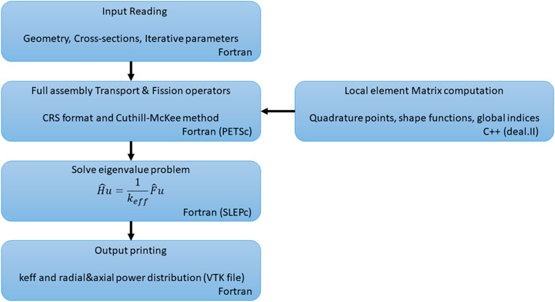
Figure 1. KANECS calculation scheme.

4 Numerical results

In this section, the KAIST (Cho, 2000) and C5G7 (Lewis et al., 2003) benchmarks are simulated to verify the KANECS’ capabilities. For verification, the computational results are compared using other deterministic neutron transport codes, PARAFISH (P_N) (Duran-Gonzalez et al., 2022) and AZTRAN (S_N) (Duran-Gonzalez et al., 2021) employing the same conditions (geometry, cross sections, and convergence criteria). In order to conduct a comprehensive code-to-code comparison, the following collective relative error measures are used: the $k_{\mathit{eff}}$ deviation is calculated in Equation 19a, the maximum relative error for the pin power is defined in Equation 19b, and the relative root-mean-square (RMS) disparity is shown in Equation 19c, where $N_p$ represents the total number of active pins.

$\mathrm{\Delta }{k}_{\mathit{eff}}\left[pcm\right]=10^5\left(k_{\mathit{eff}}^{\mathrm{K}\mathrm{A}\mathrm{N}\mathrm{E}\mathrm{C}\mathrm{S}}-k_{\mathit{eff}}^{\mathit{ref}}\right)(\mathrm{19a})$

${\epsilon }_{\mathit{MAX}}\left[\%\right]=\max \left(\frac{\left|P_i^{\mathrm{K}\mathrm{A}\mathrm{N}\mathrm{E}\mathrm{C}\mathrm{S}}-P_i^{\mathit{ref}}\right|}{P_i^{\mathit{ref}}}\times 100\right)(\mathrm{19b})$

${\epsilon }_{\mathit{RMS}}\left[\%\right]=\sqrt{\frac{1}{N_p}{\displaystyle \sum _{i=1}^{N_p}}{\left(\frac{P_i^{\mathrm{K}\mathrm{A}\mathrm{N}\mathrm{E}\mathrm{C}\mathrm{S}}-P_i^{\mathit{ref}}}{P_i^{\mathit{ref}}}\times 100\right)}^2}(\mathrm{19c})$

Finally, all the calculations were performed with convergence criteria set to $10^{-7}$ for the neutron flux and $10^{-6}$ for $k_{\mathit{eff}}$. All codes were executed in a workstation with an AMD EPYC 7543 Processor and a 200 GB RAM, using a single processor core.

4.1 KAIST 3A benchmark

The KAIST 3A benchmark features a simplified Pressurised Water Reactor (PWR) with a MOX-loaded core, it is part of a series developed by the KAIST Nuclear Reactor Analysis and Particle Transport Laboratory (Cho, 2000). The core comprises two types of fuel assemblies: UOX (UOX-1 with 2.0% enrichment and UOX-2 with 3.3% enrichment) and MOX. A reflector and a steel baffle surround the fuel assemblies. Each assembly constitutes a 17 × 17 lattice design with a width of 21.42 cm and a pin-cell pitch of 1.26 cm. This benchmark provides 7-group pin-cell homogenized cross sections (Cho, 2000) based on the HELIOS 34 group structure, including UOX, MOX, guide tubes, fuel rods, control rods, poison rods, a baffle, and a reflector. The core layout of the KAIST 3A benchmark is illustrated in Figure 2.

Figure 2

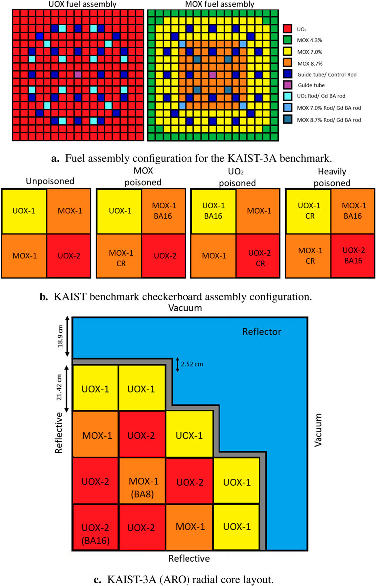
Figure 2. KAIST-3A benchmark geometry. (A) Fuel assembly configuration for the KAIST-3A benchmark. (B) KAIST benchmark checkerboard assembly configuration. (C) KAIST-3A (ARO) radial core layout.

4.1.1 KAIST 3A assembly cases

As a first verification exercise, the different fuel assembly types (Figure 2A) were analyzed, consisting of 6 UOX and 3 MOX assemblies, with variations in the number of burnable absorbers and control rods. The results obtained for all the different fuel types are summarized in Table 1. First, it could be observed that KANECS demonstrated excellent agreement for assemblies without control rods or burnable absorbers, with RMS errors of less than 0.79% and $k_{\mathit{eff}}$ deviation below 42 pcm compared to other transport codes. However, notable differences arose as heterogeneity increased (burnable absorbers and control rods), obtaining RMS errors of up to 1.22% (UOX-1-BA16) and $k_{\mathit{eff}}$ deviation around 1773 pcm (UOX-2-CR). In addition, as expected, the highest differences are observed when compared with AZTRAN in heterogeneous models since it can accurately model the sharp gradients introduced by burnable absorbers and control rods using higher angular approximation. In contrast, the SP_N method may not capture these details accurately since it assumes smoother flux distributions, making it struggle with steep flux gradients as produced for these models where the high absorption cross section leads to steep neutron flux depressions in their vicinity. Although the RMS error differences remained within an acceptable range from 0.40% to 1.22%.

Table 1

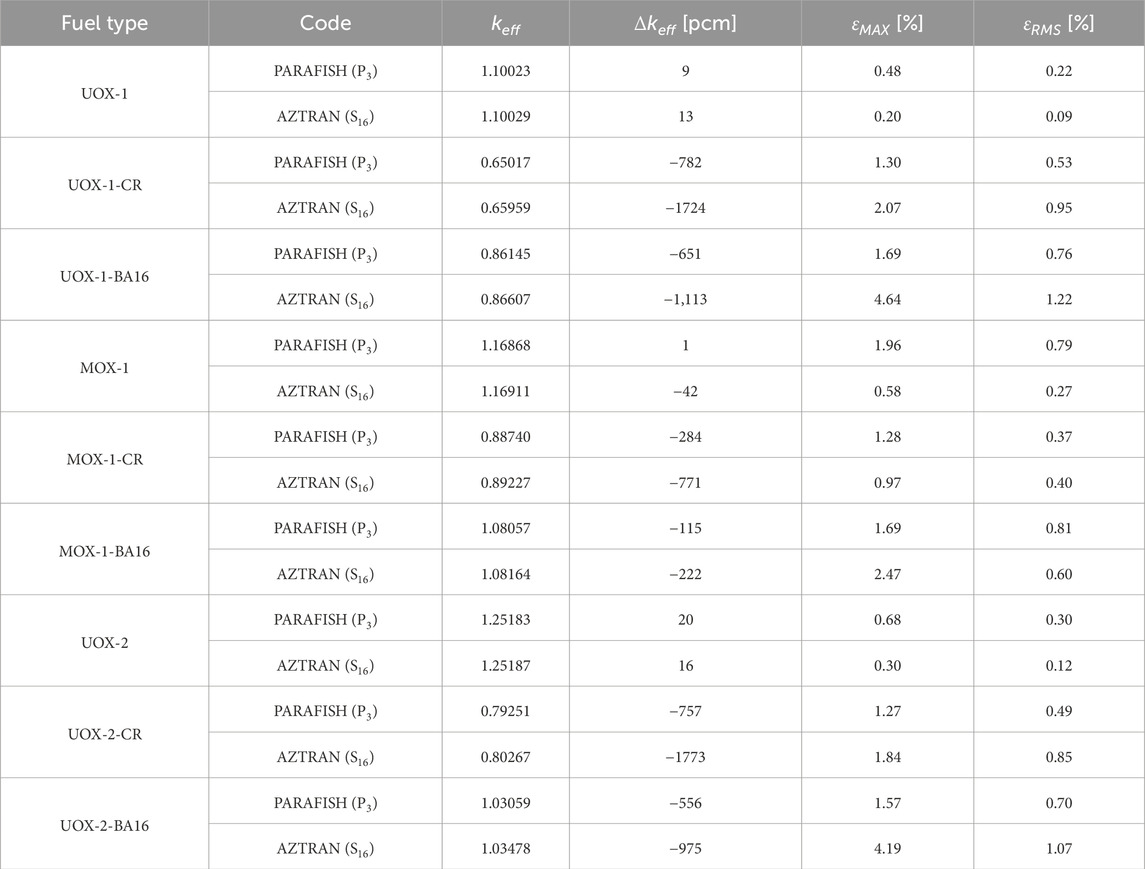
Table 1. Deviation results of KANECS SP₃ from reference codes (single-assembly KAIST).

4.1.2 KAIST 3A checkerboard cases

For the next verification, four different (UOX/MOX) checkerboard arrangements were investigated to provide a more realistic assessment. As shown in Figure 2B, the configurations have different amounts of absorbers, making them more challenging since the spectrum interface among the fuel assemblies is very strong. The checkerboard calculation results are shown in Table 2. As foreseen, the most significant discrepancies from the references occur in the poisoned cases, with RMS error differences up to 1.15% (PARAFISH) and 2.30% (AZTRAN), respectively. In addition, the highest $k_{\mathit{eff}}$ deviations were found in the Heavily poisoned assembly with 327 (PARAFISH) and 650 (AZTRAN) pcm. This is consistent with previous results, where the error increases for assemblies with strong absorbers. Despite this, the results are in reasonable agreement, with RMS error variances ranging from 0.22% to 2.30%. It is noteworthy that in some works (Yu et al., 2014; Zhang et al., 2017), the SP₃ approximation has been tested in the KAIST checkerboard benchmark, where the authors have employed approaches such as super homogenization (SPH) factors and discontinuity factors (DF) to enhance their results notably.

Table 2

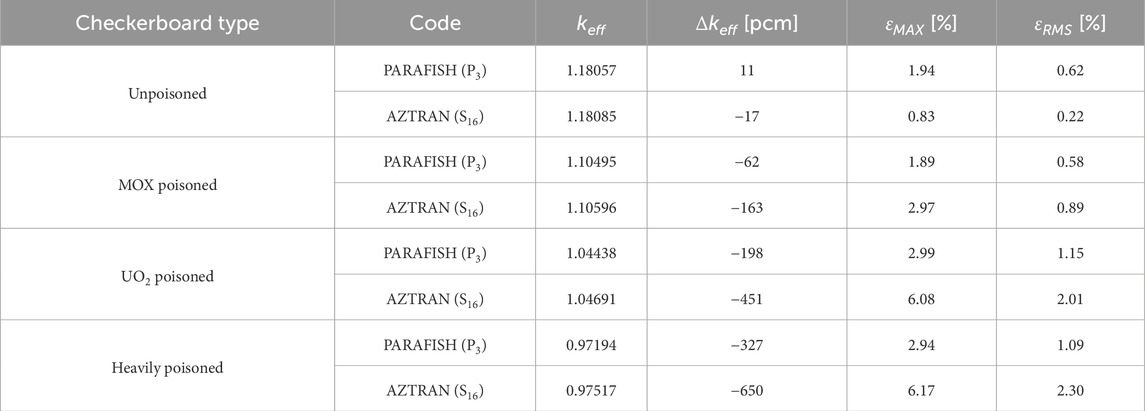
Table 2. Deviation results of KANECS SP₃ from reference codes (checkerboard KAIST).

4.1.3 2D/3D KAIST 3A ARO case

Finally, the 2D/3D KAIST 3A benchmark problems under the ARO (all control rods out) condition have been simulated. The 2D case is illustrated in the core layout depicted in Figure 2C, while the 3D case extends the same 2D radial configuration by 365.76 cm and includes axial reflectors at the top and bottom of the core, each with a width of 21.42 cm. The results of the calculation are outlined in Table 3, and the detailed pin power distribution from the KAIST 3A is illustrated in Figure 3. The results show that the $k_{\mathit{eff}}$ deviations are less than 156 and 214 pcm for the 2D and 3D cases, respectively. Furthermore, the maximum RMS discrepancy is approximately 1.07% against AZTRAN and 0.77% for PARAFISH. It is worth noting that the differences between 2D and 3D cases are minimal due to the high axial homogeneity of the core. Overall, the results align well with the transport references, especially considering that the ARO configuration is less heterogeneous than previous examples, leading to minor discrepancies. Table 4 presents the results for the 2D case compared with AZTRAN (S₁₆) for different angular approximations and finite element polynomial degree (DEG). As it can be appreciated, the accuracy improves as the angular approximation and polynomial degree increase. In this particular case, the polynomial degree plays a crucial role in reducing discrepancies, as demonstrated by the substantial reduction in the maximum relative error from 18.28% to 4.77% when moving from SP₃ with DEG 1 to SP₃ with DEG 2. Another notable observation is the enhancement in results from diffusion (SP₁) to higher angular approximations, with the RMS error reducing from 2.01% to 0.89% with an SP₇. Lastly, Table 5 shows the convergence behavior for the 2D-KAIST case with an SP₃ approximation. A noteworthy aspect is the significant difference in computing time between the eigensolvers Power iteration (PI) and Krylov-Schur. Krylov was observed to be almost four times faster than PI. Concerning the iterative solvers, GMRES and BCGS exhibited similar computing times, with GMRES requiring more inner iterations to converge but being slightly faster than BCGS. Ultimately, related to the preconditioners, the efficiency of ILU and ICC surpassed that of JACOBI and SOR, being approximately three times faster on average.

Table 3

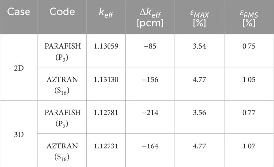
Table 3. Deviation results of KANECS SP₃ from reference codes (KAIST 3A ARO).

Figure 3

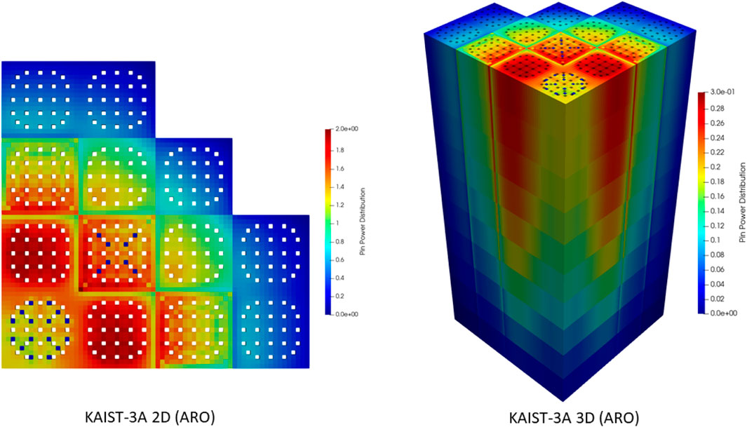
Figure 3. KAIST-3A Benchmark pin power distribution.

Table 4

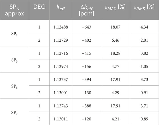
Table 4. 2D-KAIST ARO accuracy results for SP_N approximations, comparing against AZTRAN (S₁₆).

Table 5

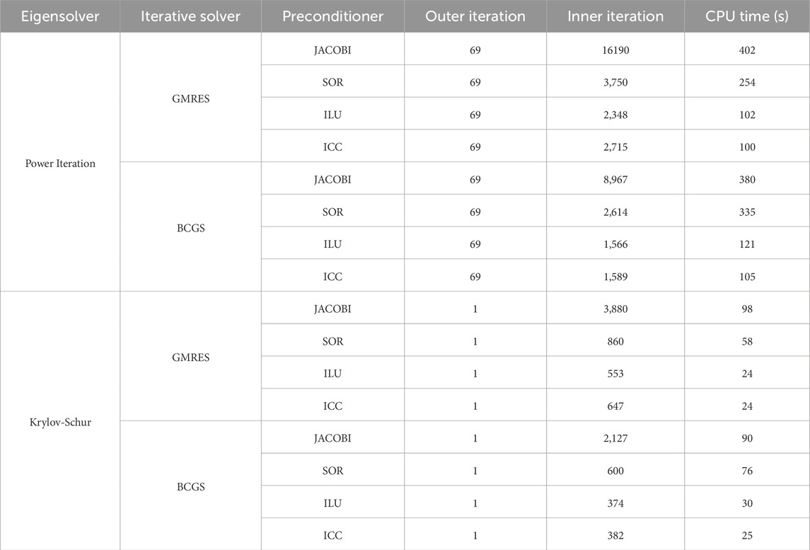
Table 5. Convergence behavior for the 2D-KAIST ARO Benchmark.

4.2 C5G7 benchmark

The C5G7 benchmark (Lewis et al., 2003), proposed by the OECD/NEA, is designed to assess the capability of modern deterministic neutron transport codes in simulating heterogeneous reactor cores with strong transport gradients and without spatial homogenization. The C5G7 configuration, represented in Figure 4, includes two types of fuel assemblies (UO₂ and MOX). Each assembly consists of a 17 × 17 pin-cell containing materials such as UO₂, 4.3% MOX, 7.0% MOX, 8.7% MOX, a fission chamber, a guided tube, and a moderator. The side length of each assembly is 21.42 cm, and the pin-cell pitch is 1.26 cm. A noteworthy aspect, as the KANECS code deals with Cartesian geometry and cannot handle circular shapes, a rectangular mesh discretization displayed in Figure 4A is employed, preserving the circular area. Further details and specifications, including the geometry and the isotropic transport corrected cross sections with 7 energy groups, can be found in (Lewis et al., 2003).

Figure 4

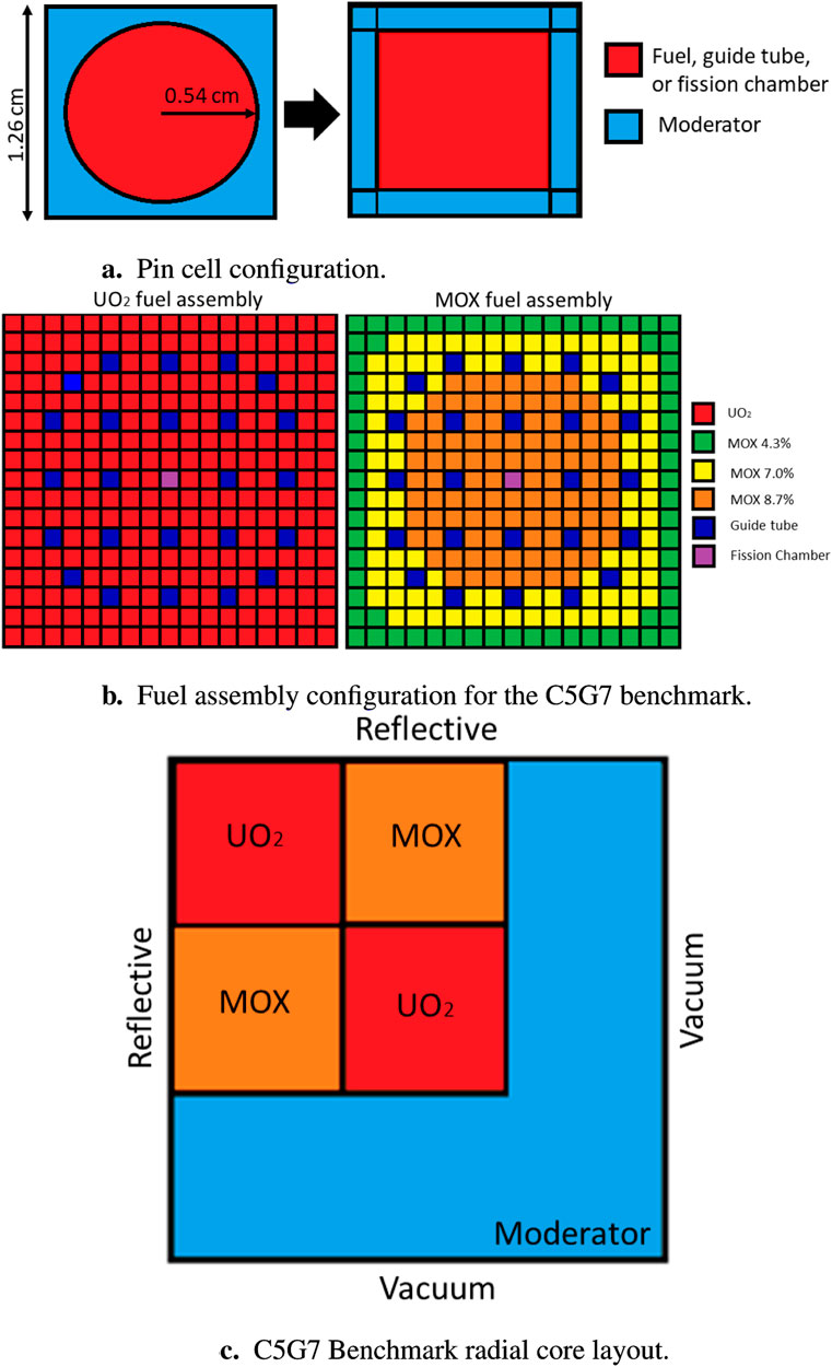
Figure 4. C5G7 benchmark geometry. (A) Pin cell configuration. (B) Fuel assembly configuration for the C5G7 benchmark. (C) C5G7 Benchmark radial core layout.

4.2.1 Assembly cases

The first exercise verification simulates the UO₂ and MOX fuel assemblies illustrated in Figure 4B. Two configurations were considered: “fully reflected” (reflective boundary conditions applied to all faces) and “partially reflected” (vacuum boundary conditions on the right and bottom and reflective boundary conditions on the top and left). Table 6 provides the calculation results. As it can be observed, the fully reflected results showed excellent concordance, the highest difference was found in the MOX assembly with an RMS error difference below 0.56% and $k_{\mathit{eff}}$ deviation less than 693 pcm. In contrast, there were significant discrepancies in the partially reflected models, especially in the UO₂ assembly, in which the maximum relative differences found were nearly 2.56%, mainly in the regions close to vacuum boundaries, although the RMS errors were below 0.97%. These differences may be caused by the Marshak Boundary Conditions applied in the SP₃ approximation, which are better suited for “diffuse boundaries” rather than fuel assemblies. Under this situation, the Marshak Boundary Conditions can lead to different flux distributions near the boundaries compared to vacuum (zero incoming flux) boundary conditions provided by the S_N method. It is worth mentioning that even though the P₃ approximation also applies the Marshak Boundary Conditions, it is still accurate since it considers more angular moments. Thus, it can better represent the flux gradients.

Table 6

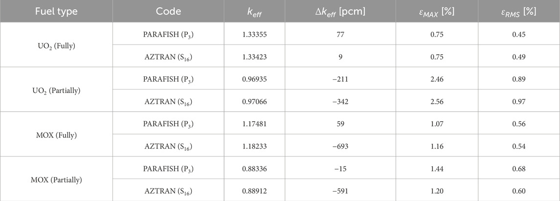
Table 6. Deviation results of KANECS SP₃ from reference codes (single-assembly C5G7).

4.2.2 C3 mini-core configuration

The following exercise involves modeling the C3 benchmark, which features a 2 × 2 mini-core configuration. This model is essentially the C5G7 model shown in Figure 4C, except that the moderator does not surround it, and the reflective boundary conditions are applied to all four faces. The results, displayed in Table 7, again showcase the consistency with the previous results. The solution produced a good agreement with the references. KANECS closely aligns with PARAFISH, obtaining differences of approximately 53 pcm for the $k_{\mathit{eff}}$ and 0.64% for the RMS error. Additionally, compared with AZTRAN, KANECS show differences of 304 pcm and 0.77%.

Table 7

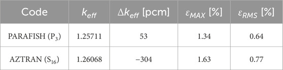
Table 7. Deviation Results of KANECS SP₃ from Reference Codes (C3 minicore).

4.2.3 2D/3D C5G7 benchmark

At last, the 2D/3D C5G7 benchmarks were analyzed. The 2D configuration is shown in Figure 4C. Regarding the 3D configuration, the fuel assemblies are extended 192.78 cm in the z-direction with an additional 21.42 cm of moderator material axially added at the top and bottom. The numerical results are illustrated in Table 8, with maximum eigenvalue errors of about 261 and 275 pcm for the 2D and 3D cases, respectively. Furthermore, the maximum RMS errors are found to be less than 1.10%, indicating that the results of simulating a core without spatial homogenization agree with the transport references. Lastly, Figure 5 illustrates the corresponding pin power distribution for each configuration. Concerning the sensitivity analysis of the 2D-C5G7 Benchmark’s accuracy, Table 9 displays the results obtained by varying the angular approximation and the polynomial degree compared to AZTRAN (S₁₆). As expected, the accuracy increases as the parameters grow, moving from the lowest approximation, SP₁ with DEG 1 (${\epsilon }_{\mathit{MAX}}$ = 8.50% and ${\epsilon }_{\mathit{RMS}}$ = 2.27%), to the highest approximation, SP₇ with DEG 2 (${\epsilon }_{\mathit{MAX}}$ = 3.64% and ${\epsilon }_{\mathit{RMS}}$ = 0.88%). To conclude, Table 10 depicts the convergence behavior for the 2D-C5G7 with an SP₃ approximation. As the previous results, the Krylov-Schur proved to be the most efficient eigensolver, being almost 3 times faster than the Power Iteration method. Among the iterative solvers, GMRES and BCGS demonstrated similar computational times (although GMRES required more iterations), while the ILU and ICC preconditioners achieved faster convergence compared to JACOBI and SOR.

Table 8

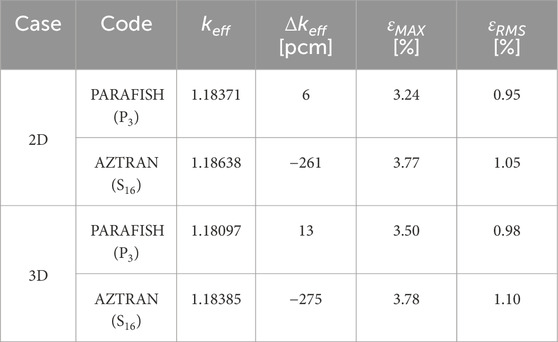
Table 8. Deviation results of KANECS SP₃ from reference codes (C5G7 benchmark).

Figure 5

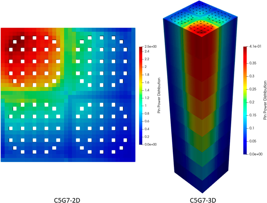
Figure 5. C5G7 Benchmark pin power distribution.

Table 9

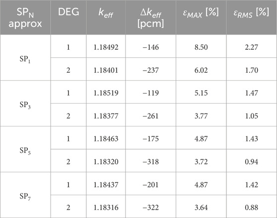
Table 9. 2D-C5G7 accuracy results for SP_N approximations, comparing against AZTRAN (S₁₆).

Table 10

Table 10. Convergence behavior for the 2D-C5G7 Benchmark.

5 Conclusion and outlook

The Karlsruhe Neutronics Core Simulator (KANECS) was recently developed and verified using the well-known benchmark problems KAIST 3A and C5G7. KANECS is based on the SP_N approximation and continuous Galerkin finite-element method (CGFEM). Furthermore, it was founded on three powerful libraries deal. ii, PETSc, and SLEPc, which together offer advanced simulation software for solving large-scale problems like the neutronic pin-by-pin analysis. The results of the KAIST-3A problems usually exhibited good concordance with respect to the transport references. However, when analyzing the checkerboard arrangements, which are very heterogeneous configurations, significant differences were found since the SP_N approximation might struggle in regions with strong flux gradients (like fuel pins adjacent to control rods or gadolinium rods). Consequently, super homogenization or discontinuity factors approaches need to be implemented as in other similar tools to enhance the results. Regarding the C5G7 benchmarks, the results show good agreement with the references despite being a more challenging problem without spatial homogenization. To summarize, KANECS was shown to provide good overall accuracy in predicting the $k_{\mathit{eff}}$ and pin power distribution fairly close to the transport approaches, with minor localized errors that do not detract significantly from the solver’s effectiveness for practical reactor simulations with a low computational cost. Moreover, the results clearly show that KANECS (SP₃) is closer to PARAFISH (P₃) than AZTRAN (S₁₆) as it was theoretically expected. Additionally, the more accurate results are obtained as the angular approximation and polynomial degree increase. This is particularly noticeable in the transition from the diffusion approximation (SP₁) to the SP₃ approximation. However, with higher-order approximations, such as SP₅ and SP₇, the accuracy only improves slightly compared to SP₃. Finally, when selecting the iterative solvers, the computing time results demonstrated that the Krylov-Schur eigensolver is much more powerful than the Power Iteration method. Meanwhile, GMRES or BCGS solvers yield similar results, with GMRES being slightly faster while using either ILU or ICC preconditioner converging more rapidly than SOR and JACOBI. Future efforts will be devoted to implement the matrix-free method, which will reduce computational memory usage by iteratively forming the matrix without explicitly forming it. Furthermore, an unstructured mesh implementation is also ongoing, taking advantage of the deal. II library capability to handle flexible grids. Lastly, KANECS will be extended to perform time-dependent calculations coupled with in-house core thermal-hydraulic code, such as SUBCHANFLOW and TWOPORFLOW.

Data availability statement

The original contributions presented in the study are included in the article/supplementary material, further inquiries can be directed to the corresponding author.

Author contributions

JD-G: Conceptualization, Formal Analysis, Methodology, Software, Validation, Writing–original draft, Writing–review and editing. AC-M: Conceptualization, Methodology, Software, Writing–original draft, Writing–review and editing. V-HS-E: Conceptualization, Methodology, Supervision, Writing–original draft, Writing–review and editing.

Funding

The author(s) declare that financial support was received for the research, authorship, and/or publication of this article. The authors thank the HGF Program NUSAFE at KIT and the BMBF Innovation Pool SMR Initiative for the financial support. In addition, we acknowledge support by the KIT-Publication Fund of the Karlsruhe Institute of Technology.

Conflict of interest

The authors declare that the research was conducted in the absence of any commercial or financial relationships that could be construed as a potential conflict of interest.

Publisher’s note

All claims expressed in this article are solely those of the authors and do not necessarily represent those of their affiliated organizations, or those of the publisher, the editors and the reviewers. Any product that may be evaluated in this article, or claim that may be made by its manufacturer, is not guaranteed or endorsed by the publisher.

References

Ahrens, J., Geveci, B., and Law, C. (2005). “Paraview: an end-user tool for large-data visualization,” in Visualization Handbook (Burlington: Butterworth-Heinemann), 717–731.

Google Scholar

Arndt, D., Bangerth, W., Bergbauer, M., Feder, M., Fehling, M., Heinz, J., et al. (2023). The deal.II library, version 9.5. J. Numer. Math. 31, 231–246. doi:10.1515/jnma-2023-0089

CrossRef Full Text | Google Scholar

Azmy, J., and Sartori, E. (2010). Nuclear Compuational Science: A Century in Review. Springer.

Google Scholar

Babcsány, B., Pós, I., Böröczki, Z. I., and Kis, D. P. (2022). Hybrid finite-element-based numerical solution of the SP3 equations – SP3 solution of two- and three-dimensional VVER reactor problems. Ann. Nucl. Energy 173, 109117. doi:10.1016/j.anucene.2022.109117

CrossRef Full Text | Google Scholar

Balay, S., Abhyankar, S., Adams, M. F., Benson, S., Brown, J., Brune, P., et al. (2024). PETSc/TAO Users Manual. Technical Report.

Google Scholar

Beckert, C., and Grundmann, U. (2008). Development and verification of a nodal approach for solving the multigroup SP3 equations. Ann. Nucl. Energy 35, 75–86. doi:10.1016/j.anucene.2007.05.014

CrossRef Full Text | Google Scholar

Brantley, P. S., and Larsen, E. W. (2000). The simplified P3 approximation. Nucl. Sci. Eng. 134, 1–21. doi:10.13182/nse134-01

CrossRef Full Text | Google Scholar

Cho, N. Z. (2000). Benchmark Problem 3A: MOX Fuel-Loaded Small PWR Core (MOX Fuel with Zoning, 7 Group Homogenized Cells). Available online at: https://github.com/nzcho/Nurapt-Archives/tree/master/KAIST-Benchmark-Problems.

Google Scholar

Duran-Gonzalez, J., del Valle-Gallegos, E., Reyes-Fuentes, M., Gomez-Torres, A., and Xolocostli-Munguia, V. (2021). Development, verification, and validation of the parallel transport code AZTRAN. Prog. Nucl. Energy 137, 103792. doi:10.1016/j.pnucene.2021.103792

CrossRef Full Text | Google Scholar

Duran-Gonzalez, J., Sanchez-Espinoza, V. H., Mercatali, L., Gomez-Torres, A., and Valle-Gallegos, E. d. (2022). Verification of the parallel transport codes parafish and AZTRAN with the TAKEDA benchmarks. Energies 15, 2476. doi:10.3390/en15072476

CrossRef Full Text | Google Scholar

Ferraro, D., García, M., Valtavirta, V., Imke, U., Tuominen, R., Leppänen, J., et al. (2020). Serpent/subchanflow pin-by-pin coupled transient calculations for a pwr minicore. Ann. Nucl. Energy 137, 107090. doi:10.1016/j.anucene.2019.107090

CrossRef Full Text | Google Scholar

Fontenla, Y., Vidal-Ferràndiz, A., Carreño, A., Ginestar, D., and Verdú, G. (2024). FEMFFUSION and its verification using the C5G7 benchmark. Ann. Nucl. Energy 196, 110239. doi:10.1016/j.anucene.2023.110239

CrossRef Full Text | Google Scholar

Gelbard, E. M. (1960). Application of the Spherical Harmonics Method to Reactor Problems. Technical Report WAPD-BT-20. Pittsburgh: Bettis Atomic Power Laboratory.

Google Scholar

Hamilton, S. P., and Evans, T. M. (2015). Efficient solution of the simplified PN equations. J. Comput. Phys. 284, 155–170. doi:10.1016/j.jcp.2014.12.014

CrossRef Full Text | Google Scholar

Hébert, A. (2010). Mixed-dual implementations of the simplified method. Ann. Nucl. Energy 37, 498–511. doi:10.1016/j.anucene.2010.01.006

CrossRef Full Text | Google Scholar

Lewis, E. E., and Miller, W. F. (1993). Computational Methods of Neutron Transport. American Nuclear Society, Inc.

Google Scholar

Lewis, E. E., Tsoulfanidis, N., and Smith, M. A. (2003). Benchmark on Deterministic Transport Calculations without Spatial Homogenization. NEA/NSC/DOC.

Google Scholar

Lo Muzio, S., and Seubert, A. (2024). Implementation of the steady state simplified P3 (SP3) transport solver in the finite element neutronic code FENNECS, part 1: theory. Ann. Nucl. Energy 200, 110303. doi:10.1016/j.anucene.2023.110303

CrossRef Full Text | Google Scholar

Muñoz-Peña, G., Galicia-Aragon, J., Lopez-Solis, R., Gomez-Torres, A., and del Valle-Gallegos, E. (2023). Verification and validation of the SPL module of the deterministic code AZNHEX through the neutronics benchmark of the CEFR start-up tests. J. Nucl. Eng. 4, 59–76. doi:10.3390/jne4010005

CrossRef Full Text | Google Scholar

Roman, J. E., Campos, C., Dalcin, L., Romero, E., and Tomas, A. (2024). SLEPc Users Manual. D. Sistemes Informàtics i Computació. Tech. Rep. DSIC-II/24/02 - Revision 3.21. Universitat Politècnica de València.

Google Scholar

Yu, L., Lu, D., and Chao, Y.-A. (2014). The calculation method for SP3 discontinuity factor and its application. Ann. Nucl. Energy 69, 14–24. doi:10.1016/j.anucene.2014.01.032

CrossRef Full Text | Google Scholar

Zhang, B., Wu, H., Liand, Y., Cao, L., and Shen, W. (2017). Evaluation of pin-cell homogenization techniques for PWR pin-by-pin calculation. Nucl. Sci. Eng. 186, 134–146. doi:10.1080/00295639.2016.1273018

CrossRef Full Text | Google Scholar

Zienkiewicz, O., Taylor, R., and Zhu, J. (2005). The Finite Element Method: Its Basis and Fundamentals. Butterworth-Heinemann.

Google Scholar