Two-layer optimization model of distribution network line loss considering the uncertainty of new energy access

The integration of a distributed generator (DG) into the distribution network alters the topology structure and power flow distribution, subsequently causing changes in network loss. Moreover, existing distribution network optimization methods face high computational complexity, low efficiency, and susceptibility to local optima. This article proposes a scenario generation method using a generative adversarial network (GAN) to handle the uncertainty associated with DGs and constructs a two-layer optimization model for the distribution network. The upper layer model determines the installation location and capacity of distributed power and energy storage systems with the lowest economic cost. The lower layer model establishes an optimization model, including wind, solar, and storage, with active power network loss and voltage deviation as objective functions. Both layers are solved using the Improved Whale Optimization algorithm (IWOA). Then, the IEEE-33 node distribution system was taken as a simulation example to verify the effectiveness and superiority of the proposed model and algorithm.

1 Introduction

To achieve the dual-carbon goal, the State Grid Corporation has proposed a plan to build a new power system to promote new energy as the dominant source of energy. New energy includes clean energy, such as wind and solar energy, which are connected to the distribution network in the form of distributed power sources (Zhang and Shao, 2017; Ma et al., 2022; Sultana et al., 2016). Connecting distributed power sources helps improve the reliability and flexibility of the power grid while reducing energy loss. However, connecting DGs to the distribution network affects the distribution network’s topology and power flow distribution due to the DG uncertainty, leading to changes in network losses (Zhang and Shao, 2017; Wang et al., 2017; Wu et al., 2023). Battery energy storage systems (BESSs), due to their advantages of being able to quickly and flexibly control the charging and discharging of energy, can effectively improve the voltage and grid loss of distribution networks containing DGs, benefiting the safe and stable operation of the distribution network. Therefore, it is necessary to optimize the two-layer model of wind and solar storage and distribution networks while taking uncertainty into account.

Scholars have conducted optimization research on distribution networks by constructing single-layer models and adopting artificial intelligence methods. Xie et al. (2021) and Wang et al. (2021) employed the clustering method and optimized the multi-classification correlation vector machine algorithm to study the line loss in low-voltage station areas in the distribution network, achieving fast convergence and accuracy. Huo et al. (2023) investigated the impact of distributed photovoltaic access on distribution network loss and used improved gray correlation analysis and stacking algorithms to study the prediction of distribution network line loss. Wu et al. (2020) and Feng et al. (2023) utilized probabilistic methods to evaluate line loss and energy loss of distribution networks. By employing the Gaussian mixture model, a highly accurate mean value of line loss and a comprehensive probability distribution of line loss can be obtained. Yao et al. (2019) employed the gradient lifting decision tree method to predict the line loss rate of the distribution network. Hu et al. (2022) utilized data from the power information acquisition system to establish a line loss calculation model based on the convolutional neural network, thereby determining the line loss interval. Pegado et al. (2019) introduced the binary particle swarm method and created a new S-function to control the particle change rate, which helps reduce the power loss in the distribution network. Li et al. (2017) proposed a calculation method for distribution network line loss based on process state characteristics, considering factors such as three-phase imbalance and DG access to the distribution network. Wang H.j. et al. (2023) addressed the problems of incomplete real-time monitoring data for electrical parameters and topology changes of distribution network nodes and proposed a line loss calculation method of a distribution network based on random forest and kernel ridge regression. However, the above-mentioned distribution network optimization methods based on a single-layer model still face high computational complexity, low computational efficiency, and a tendency to become stuck in local optimums.

With the development of new technologies such as DGs, electric vehicles (EVs), and energy storage, the planning of distribution networks has become more complex. Based on the aforementioned research findings, Liu et al. (2022) comprehensively considered the impact of DGs and EVs on the distribution network. It constructs a bi-level planning operation model that takes into account the correlation of DG power generation and EV demand response and takes the “transportation network-distribution network” as the research object to verify the model. Chen et al. (2024) considered the interests of the distribution network and microgrid, constructed a two-layer optimal scheduling model of the distribution network based on a master-slave game, and used particle swarm optimization to solve the model. Liao et al. (2024) proposed a two-layer optimal configuration method for distributed photovoltaic (DPV) and energy storage system (ESS) based on IDEC-K cluster and solved by non-dominant sequencing genetic algorithm II (NSGA-II). Zhang et al. (2022) proposed a source–grid–load–reservoir two-layer co-programming model of active distribution network (ADN) with soft open point (SOP), which is optimized by an improved particle swarm optimization algorithm.

Additionally, the intermittent and random nature of power output from high proportions of renewable energy sources connected to the distribution network poses significant challenges to the safe and stable operation of the network. Therefore, how to consider the uncertainty of power output from high proportions of renewable energy sources and take into account economy and power quality for reasonable planning of the distribution network is an urgent issue to be addressed.

As for the uncertainty of renewable energy output, researchers have conducted research from three aspects: robust optimization methods (Dai et al., 2024), traditional probabilistic modeling methods (Xun et al., 2022), and scenario generation techniques (Yuanze et al., 2021). The robust optimization method is too conservative and cannot balance the economy and security of the scheme well. Both traditional probabilistic modeling methods and scenario generation techniques assume that the data obey a specific probability distribution in advance, and the modeling process is cumbersome. In addition, large errors may occur in the parameter fitting process, resulting in poor quality of the generated scenarios. However, the generative adversarial network (GAN) has attracted much attention because it does not require assumptions about the data distribution and can directly learn the data distribution from historical data and generate new data samples (Liu et al., 2023). Yuan et al. (2023) proposed a deeply renewable scenario generation model that uses a style-based generative adversarial network to generate accurate and reliable day-ahead scenarios directly from historical data through different levels of scenario style control and mixing. Cai et al. (2023) proposed a two-layer coordinated optimal scheduling method based on GAN scenario generation. The improved coati optimization algorithm (COA) is used to solve the proposed optimization problem. Zhang et al. (2024) proposed an improved PV power generation method with a gradient penalty to solve the problems of over-reliance on statistical assumptions and unstable model training in the existing PV scenario generation methods.

Therefore, this article uses the generative adversarial network (GAN)-based generation scenario method to deal with the uncertainty associated with a high proportion of renewable energy sources. Furthermore, a two-layer optimization model for line loss in wind-solar-storage integrated distribution networks based on an improved whale algorithm is constructed. Based on the IEEE-33 node distribution network system, the effectiveness and superiority of the proposed model and method are verified.

2 Generative adversarial network scenario generation

2.1 The structure of a generative adversarial network

Traditional uncertainty handling methods are obtained by sampling from probability distributions, but the probability distribution models obtained through sample fitting often fail to accurately capture complex probabilistic characteristics. This makes it difficult for the samples processed for uncertainty to accurately simulate the actual output of wind and solar power. Therefore, this article adopts GAN for scenario generation of wind and solar power uncertainty (Liu et al., 2023).

A GAN is a deep-learning model proposed by Goodfellow in 2014 that can effectively learn the complex probability distribution of historical data in distributed generation power and generate new data samples with similar characteristics. The training process of a GAN consists of a generator and discriminator (Shao et al., 2019; Yi et al., 2024). The generator generates forged samples and improves its discrimination ability by minimizing the loss function of the discriminator. The discriminator receives real samples and forged samples at the same time, distinguishes them, and improves the authenticity of the generated samples by minimizing the loss function of the generator. Through iterative training, the generator and discriminator are continuously optimized in the mutual game, and finally, the generator can generate new samples with high fidelity. The principle is shown in Figure 1.

Figure 1

Figure 1. Schematic diagram of GAN.

In the scenario generation for high-penetration renewable energy output, the historical data of wind and photovoltaic power generation is used as the training set x. G takes random noise z as input to simulate and generate output data of wind and solar x' = G(z). D receives output data of the real wind and solar and the data generated by G. The loss functions of the two neural networks G and D in GAN are expressed in Equation 1.

$\begin{array}{l}Los{s}_G=-E_{x^{\prime }-p\left(x^{\prime }\right)}\left[D\left(x^{\prime }\right)\right]\\ Los{s}_D=-E_{x-p\left(x\right)}\left[D\left(x\right)\right]+E_{x^{\prime }-p\left(x^{\prime }\right)}\left[D\left(x^{\prime }\right)\right]\end{array},(1)$

where $Los{s}_G、Los{s}_D$ are the loss functions of G and D, respectively. E denotes the expected value of the corresponding sample. D(x') is the probability that the generated data x' are judged to be true in D. D(x) represents the probability that the real data x are discriminated to be true in D.

The objective function of GAN is to obtain a Nash equilibrium point during the game between G and D. The minimax game model is expressed as Equation 2:

${\min }_G{\max }_{D}V\left(D,G\right)=E_{x-p\left(x\right)}\left[D\left(x\right)\right]-E_{x^{\prime }-p\left(x^{\prime }\right)}\left[D\left(x^{\prime }\right)\right].(2)$

2.2 WGAN-GP

The training process of GAN usually requires a large amount of data and computing resources and may encounter training instability problems, such as pattern collapse and gradient disappearance. Better stability during the training process is provided by using the Wasserstein GAN framework with an increased gradient penalty, which replaces JS divergence with Wasserstein distance.

The Wasserstein distance is defined in Equation 3:

$W_{\left(p_x,p_{x^{\prime }}\right)}=\underset{‖f_D‖L\le 1}{\sup }{E}_{p\left(x\right)}\left[D\left(x\right)\right]-E_{p\left(x^{\prime }\right)}\left[D\left(x^{\prime }\right)\right],(3)$

where $‖f_D‖L\le 1$ indicates that discriminator D needs to satisfy 1-Lipschitz continuity.

The gradient penalty is defined in Equation 4:

$GP{|}_{\widehat{x}}=\lambda E_{\widehat{x}-p\left(\widehat{x}\right)}\left[{\left({‖{\nabla }_{\widehat{x}}D\left(\widehat{x}\right)‖}_2-1\right)}^2\right],(4)$

where $\widehat{x}=\epsilon x+\left(1-\epsilon \right)x^{\prime },\epsilon \sim U\left[0,1\right]$. ${‖•‖}_2$ denotes two norms. λ represents the weight coefficient of the gradient penalty term.

The objective function of WGAN-GP is transformed by Equation 5:

${\min }_G{\max }_{D}V\left(G,D\right)=E_{x-p\left(x\right)}\left[D\left(x\right)\right]-E_{x^{\prime }-p\left(x^{\prime }\right)}\left[D\left(x^{\prime }\right)\right]-\lambda E_{\widehat{x}-p\left(\widehat{x}\right)}\left[{\left({‖{\nabla }_{\widehat{x}}D\left(\widehat{x}\right)‖}_2-1\right)}^2\right].(5)$

After the above optimization, the objective function of WGAN-GP is transformed to minimize the Wasserstein distance between the generated data and the real data, and a gradient penalty term is added to ensure the training stability of the generator and discriminator. Therefore, the wind/ solar output scenario generation method based on WGAN-GP can more effectively capture the characteristics of data distribution, thereby generating more realistic and diversified data samples. This provides strong technical support for the simulation and prediction of wind/solar output scenarios.

2.3 Training results

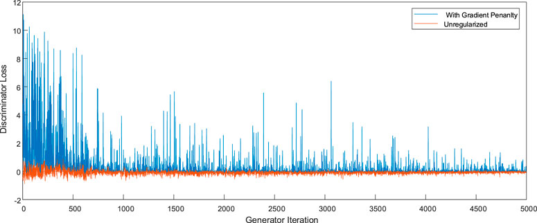
The output data of 96 points of wind power and photovoltaic power generation in 1 day are taken as the input of D in WGAN-GP, respectively. After training, the scenario’s combined output can be generated, and the training results are shown in Figures 2, 3. During the training process, the variation curve of the Wasserstein distance between the generated and the real scenarios with the training times is shown in Figure 4.

Figure 2

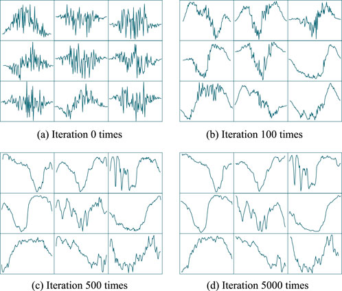
Figure 2. Wind output curve. (A) Iteration 0 times. (B) Iteration 100 times. (C) Iteration 500 times. (D) Iteration 5000 times.

Figure 3

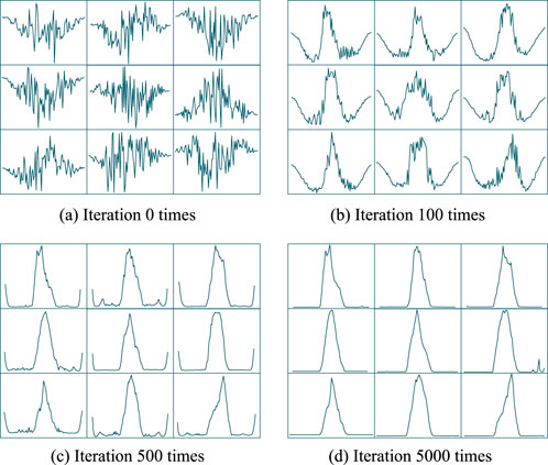
Figure 3. Solar output curve. (A) Iteration 0 times. (B) Iteration 100 times. (C) Iteration 500 times. (D) Iteration 5000 times.

Figure 4

Figure 4. Variation curve of Wasserstein distance with training times.

In Figures 2, 3, the horizontal direction of the picture represents the time scale, and the vertical direction is the standard value of wind and solar output. The generated wind and solar output data take 15 min as the time interval, and the output curve contains 96 data points. Figures 2A–D represent the wind output curves of the model learning 0, 100, 500, and 5,000 times, respectively. Figures 3A–D represent the solar output curves of the model learning 0, 100, 500, and 5,000 times, respectively. Each subgraph contains nine wind and solar output curves generated by generator G.

At the beginning of training, because generator G has not learned the wind and solar output data, the output data are generated by random noise and do not have the output characteristics of wind and solar, as shown in Figures 2A, B. When training is performed 100 times, generator G captures some output characteristics of the wind and solar data, and the generated output data are periodically transformed. At 500 times, generator G learns the periodic change of the wind and solar output, and the generated data gradually stabilize and no longer change drastically. They show the periodic change characteristics of the wind and solar output. At 5,000 times, because generator G has fully captured the intrinsic characteristics of wind and solar output and reached a Nash equilibrium with the discriminator D, the generated output curve is relatively smooth. The generated photovoltaic output curve shows that the output is concentrated during the daytime period, while the output is 0 at night. The generated output curve of wind power shows the characteristics of concentrated output at night, but the overall fluctuation is large. These results are consistent with the characteristics of wind and solar output in engineering practice. They indicate that the model proposed can accurately learn and capture the output characteristics of wind and solar.

It can be seen from Figures 2–4 that the fitting error of the discriminator D to the Wasserstein distance is large in the initial stage of training because generator G has not fully learned the output characteristics of wind and solar. With continuous training, generator G gradually mines the output characteristics of wind and solar, which makes the coincidence between the output data of generated wind and solar and the measured data gradually increase. At this time, the Wasserstein distance begins to decrease and tends to be stable. When generator G has fully learned the output characteristics of the scenario, the Wasserstein distance fluctuates stably around 0. At this time, generator G and the discriminator D have reached a Nash equilibrium, and the discriminator D can no longer distinguish the difference between the generated data and the real data. Finally, the WGAN-GP training converges.

In order to test the quality of the WGAN-GP generation scenarios, the cumulative probability distribution functions of the generation sample and the historical sample are plotted, as shown in Figures 5, 6. It can be seen that the cumulative probability distributions of the two are quite close, which shows that the wind/solar data generated based on WGAN-GP are reasonable.

Figure 5

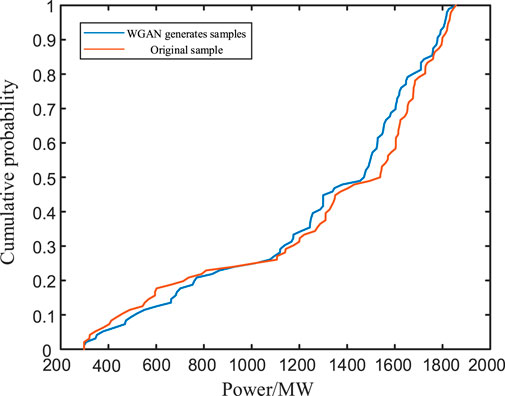
Figure 5. Cumulative probability distribution functions of wind generation samples and historical samples.

Figure 6

Figure 6. Cumulative probability distribution functions of solar generation samples and historical samples.

To further illustrate the computational complexity and accuracy of the generated scenarios, some unlearned datasets were selected and compared with the traditional Monte Carlo sampling scenario generation method. Statistics were performed on the generated data and the real data, and the results are shown in Table 1. The scenario evaluation indicators in Table 1 are as follows:

Table 1

Table 1. Generate evaluation indicators for scenarios under.

The root mean square error (RMSE) can reflect the deviation between the output value of the generated wind and solar and the true value. The lower the RMSE value determined by Equation 6, the higher the fitting accuracy of the generated data.

$X_{\text{RSME}}=\sqrt{\frac{1}{n}{\displaystyle \sum _i^n}{\left(y_i-{\widehat{y}}_i\right)}^2,}(6)$

where $y_i$ is the output value for the real scenario. ${\widehat{y}}_i$ is the output value of the generated wind and light. n represents the number of pieces $y_i$. $\overline{y}$ is the average value of $y_i$.

The mean absolute error (MAE) can verify the difference between the output value of the generated wind and solar and the true value by measuring the average size of the error. The smaller the value of MAE determined by Equation 7, the closer the generated data are to the true value.

$X_{\text{MAE}}=\frac{1}{n}{\displaystyle \sum _i^n}\left|y_i-{\widehat{y}}_i\right|.(7)$

The mean absolute percentage error (MAPE) can be used to describe the difference between the generated value and the true value by the percentage error. The smaller the MAPE value determined by Equation 8, the closer the generated data are to the true value.

$X_{\text{MAPE}}=\frac{1}{n}\left.{\displaystyle \sum _i^n}\right|\frac{y_i-{\widehat{y}}_i}{y_i}|\times 100\%.(8)$

When Table 1 is combined with Figures 5, 6, it can be seen that the cumulative distribution function of the data generated by WGAN-GP is close to the distribution of the real sample. The proposed method can obtain the distribution characteristics of wind power and photovoltaic output data through implicit learning and obtain data that are closer to the real wind and solar output. The result illustrates the effectiveness of the proposed method in terms of probability distribution.

2.4 K-means clustering scenario reduction

In order to reduce the difficulty of solving the planning model later, the k-means clustering algorithm is used to reduce the scenarios (Zhang et al., 2021). The specific steps are as follows: (1) Arbitrarily select k scenarios from the matrix N as the clustering center. (2) By calculating the Euclidean distance, assign the remaining data points to the nearest cluster centered on selected cluster centers and then recalculate the cluster centers of these clusters for comparison and updating with the previous data. (3) Repeat the above steps until the cluster centers no longer change.

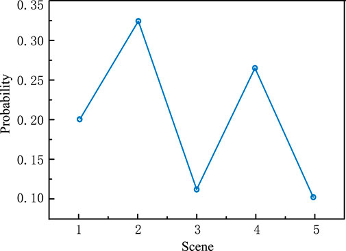
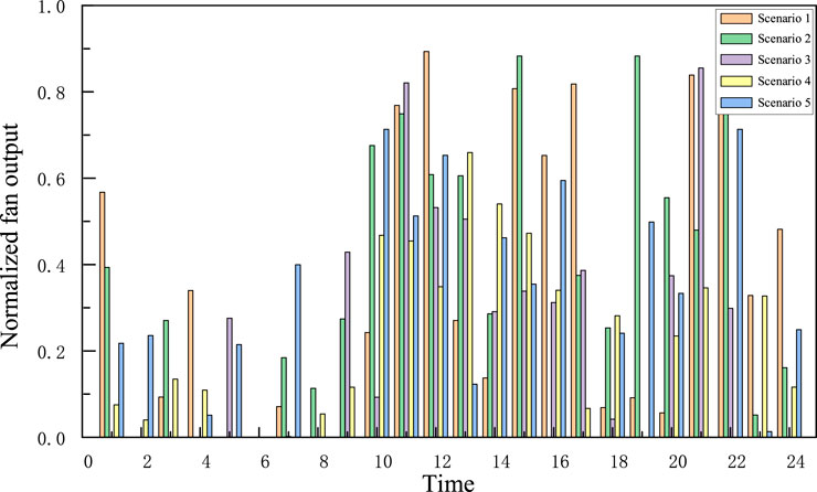
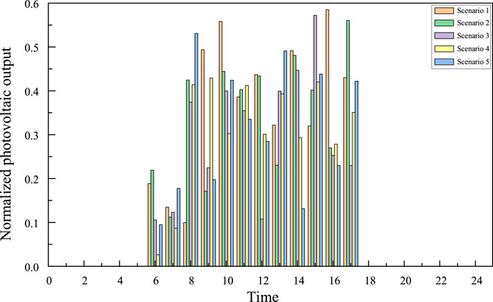
K-means clustering is used for scenario reduction and normalization to generate five typical scenarios with scenery output. The probability of each scenario is shown in Figure 7, and the scenario reduction results are shown in Figures 8, 9.

Figure 7

Figure 7. Probability graph of typical scenarios.

Figure 8

Figure 8. Normalized fan output diagram.

Figure 9

Figure 9. Normalized PV output diagram.

3 Dual-layer optimization model for power distribution network

3.1 Upper layer model

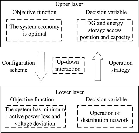
The upper-level model considers the system economic cost of the distribution network planning, aiming for the optimal annual comprehensive cost. In the model, the location and capacity of DGs and BESSs are planned.

3.1.1 Objective function

$\min C_{\mathrm{p}}=\min \left(C_{\mathrm{r}}+C_{\mathrm{i}}\right),(9)$

where $C_{\mathrm{p}}$ is the total cost at the planning level, $C_{\mathrm{r}}$ is the operating costs, and $C_{\mathrm{i}}$ is the investment costs of DGs and BESSs (Xun et al., 2022) (Equation 9).

(1) Operating costs are determined as shown in Equation 10:

$C_{\mathrm{r}}=C_{\mathrm{G}}+C_{\text{loss}}+C_{\text{DG}}+C_{\text{BS}},(10)$

where $C_{\mathrm{G}}$, $C_{\text{loss}}$, $C_{\text{DG}}$, and $C_{\text{BS}}$ represent purchase cost and network loss cost of the main network electricity and operation fees of wind, photovoltaic, and energy storage, respectively. The specific formulas for each indicator can be found in Shao et al. (2019).

(2) Investment costs determined as shown in Equation 11:

$C_{\mathrm{i}}=\frac{r{\left(1+r\right)}^n}{{\left(1+r\right)}^n-1}\left({\displaystyle \sum _{i=1}^{N_{\text{DG}}}}{c}_{\text{inv},\text{DG}}{P}_{i,\text{DG}}+{\displaystyle \sum _{i=1}^{N_{\text{BS}}}}{c}_{\text{inv},\text{BS}}{E}_{i,\text{BS}}\right),(11)$

where $c_{\text{inv}}$ and N are the unit capital investment cost and installation quantity, respectively; $P_{i,\text{DG}}$ and $E_{i,\text{BS}}$ are the installed capacities of the DG and BESS at node i. n is the economic service life; r is the annual return rate.

3.1.2 Constraints

(1) Total investment cost constraints are determined as shown in Equation 12:

$C_{\text{inv},\text{DG}}+C_{\text{inv},\text{BS}}\le C_{\text{inv},\text{total}},(12)$

where $C_{\text{inv},\text{total}}$ is the upper limit of total investment cost.

(2) Capacity constraints are determined as shown in Equation 13:

$\left\{\begin{array}{l}0\le P_{i,\text{DG}}\le P_{i,\text{DG}}^{\max }\\ 0\le E_{i,\text{BS}}\le E_{i,\text{BS}}^{\max }\end{array}\right.,(13)$

where $P_{i,\text{DG}}^{\max }$ and $E_{i,\text{BS}}^{\max }$ represent the maximum capacity of the DG and BESS installed at node i, respectively.

3.2 Lower level model

The lower-level model is established with the objective functions of minimizing active power losses and voltage deviations in the distribution network, creating an operational model for the distribution network that includes wind, photovoltaic, and storage.

3.2.1 Objective function

(1) Minimum active power losses are determined as shown in Equation 14:

$\begin{array}{l}\min P_{\text{loss}}=f_1=\frac{r\mathrm{L}}{3U^2}[P_{\mathrm{L}}^2+Q_{\mathrm{L}}^2\left.+\left(P_{\text{DG}}^2+Q_{\text{DG}}^2-2P_{\mathrm{L}}{P}_{\text{DG}}-2Q_{\mathrm{L}}{Q}_{\text{DG}}\right)\left(\frac{l}{\mathrm{L}}\right)\right]\end{array},(14)$

where r is the single-phase resistance. U is the phase voltage. $P_{\mathrm{L}}$ and $Q_{\mathrm{L}}$ are the active power and reactive power consumed by the load, respectively. $P_{\text{DG}}$ and $Q_{\text{DG}}$ are the active power and reactive power output produced by the distributed power source. L is the total length of the distribution line. l is the distance between the power source and the DG.

(2) The minimum voltage deviation is determined as shown in Equation 15:

$\min \Delta V=f_2={\displaystyle \sum _{i=1}^N}\left|V_i{-V}_{\mathrm{r}}\right|,(15)$

where N represents the total number of nodes. $V_i$ is the actual voltage value of the node i. $V_{\mathrm{r}}$ is the rated voltage of the distribution network.

(3) Target weight settings (Wang Y. F. et al., 2023; Shahraki et al., 2023) are determined as shown in Equation 16:

$f=\alpha f_1+\beta f_2(16)$

according to Deb and Jain (2014). $\alpha$ and $\beta$ are the weight coefficients of objective functions 1 and 2, respectively, with $\alpha +\beta =1$, and $\alpha =0.4$, $\beta =0.6$.

3.2.2 Constraints

(1) System power balance constraints are determined as shown in Equation 17:

$\left\{\begin{array}{l}{P}_{\mathrm{G}i}+P_{\text{DG}i}=P_{\mathrm{L}i}+V_i{\displaystyle \sum _{j=1}^N}{V}_j\left(G_{ij}\cos {\theta }_{ij}+B_{ij}\sin {\theta }_{ij}\right)\\ Q_{\mathrm{G}i}+Q_{\text{DG}i}=Q_{\mathrm{L}i}+V_i{\displaystyle \sum _{j=1}^N}{V}_j\left(G_{ij}\cos {\theta }_{ij}-B_{ij}\sin {\theta }_{ij}\right)\end{array}\right.,(17)$

where $P_{\mathrm{G}i}$ and $Q_{\mathrm{G}i}$ are the active and reactive power injected by the generator at node i, respectively. $P_{\text{DG}i}$ and $Q_{\text{DG}i}$ are the active and reactive power of the distributed generator at the i node, respectively. $P_{\mathrm{L}i}$ and $Q_{\mathrm{L}i}$ are the active and reactive power injected by the load at node i, respectively. $V_i$ and $V_j$ are the voltages at the distribution input node i and output node j, respectively. $G_{ij}$ and $B_{ij}$ are the conductance and susceptance between nodes i and j, respectively. ${\theta }_{ij}$ is the phase difference between nodes i and j.

(2) Node voltage constraints are determined as shown in Equation 18:

$V_{i\min }\le V_i\le V_{i\max .}(18)$

(3) DG power output constraints are determined as shown in Equation 19:

$0\le P_{\text{DG}i}\le P_{\text{DG}i\max .}(19)$

(4) Energy storage charging and discharging power constraints are determined as shown in Equation 20:

$\left\{\begin{array}{l}{\eta }^{\text{BS}}\left(E_t^{\text{BS}}-E_{t-\Delta t}^{\text{BS}}\right)=-P_{i,t}^{\text{BS}}\Delta t\\ \left|P_{i\min }^{\text{BS}}\right|\le \left|P_{i,t}^{\text{BS}}\right|\le \left|P_{i\max }^{\text{BS}}\right|\end{array}\right.,(20)$

where ${\eta }^{\text{BS}}$ is the charge–discharge efficiency

(5) Energy storage charge and discharge state constraintsEnergy storage devices can only be in a charging or discharging state at any time t during normal operation and can be expressed as Equation 21:

$P_{i,t}^{\text{BS}1}{P}_{i,t}^{\text{BS}2}=0,(21)$

where $P_{i,t}^{\text{BS}}$ represents the charging and discharging power of energy storage device i during time period t.

4 Two-layer model solving

4.1 Basic Whale Optimization algorithm (WOA)

The Whale Optimization algorithm (WOA) is a heuristic optimization algorithm based on the hunting behavior of humpback whales in nature. Whales use different hunting strategies to find the best food location, among which there are two main hunting mechanisms: around the prey and spiral hunting. These behaviors inspire the process of searching for the optimal solution to the optimization problem.

WOA’s basic algorithm updates its search location by simulating the behavior of humpback whales. Each whale’s position update can be represented in one of two ways.

4.1.1 Behavior around prey

$X\left(t+1\right)=X_k\left(t\right)-A\cdot D,p<0.5.(22)$

where $X_k\left(t\right)$ is the current candidate solution, $A$ is the coefficient, and $D$ is the distance between the optimal solution and the current solution (Wang Y. F. et al., 2023) (Equation 22).

4.1.2 Spiral update behavior

$X\left(t+1\right)=X_k\left(t\right)+D^{\prime }\cdot e^{bl}\cdot \cos \left(2\pi l\right),p\ge 0.5,(23)$

where $b$ the control parameter of the spiral shape. $l$ is a random control parameter and ∈ [−1, 1]. $D^{\prime }$ is the distance between the current solution and the optimal solution. Where $b$ the control parameter of the spiral shape. $l$ is a random control parameter and ∈ [−1, 1]. $D^{\prime }$ is the distance between the current solution and the optimal solution. $p$ is a random number that is used to select an update policy in the range of [0,1] (Shahraki et al., 2023) (Equation 23). When $p<0.5$, the whale calculates the distance between the current solution and the optimal solution and updates the position to approach the optimal solution. At that time $p\ge 0.5$, the whale searches for prey along a spiral path, adjusting its position through an updated formula that simulates the process of hunting.

The algorithm uses these two behaviors to achieve a balance between global and local searches. Through these behaviors, the whale optimization algorithm is able to perform global and local exploration within the search space.

4.2 Improving the Whale Optimization algorithm (WOA)

On the basis of the basic WOA, an Improved Whale Optimization algorithm (IWOA) is proposed. The core of the improvement lies in the introduction of nonlinear control parameters $l$, which can be dynamically adjusted according to the number of iterations so as to achieve a more appropriate balance of global and local search at different stages and improve the convergence accuracy and algorithm performance.

4.2.1 Introduction of nonlinear control parameters

In order to better control the search behavior, nonlinear control parameters $l$ are introduced so that the whale search strategy can be gradually refined with the increase of the number of iterations, as shown in Equation 24. The corresponding parameters l in Equation 23 can be updated.

$l=a_2\cdot {\text{rand}}_1+1-\sqrt{\frac{t}{\max -\text{iter}}},(24)$

where $a_2=\sin \left(\frac{\pi }{2}\cdot \left(1-l\right)\right)$ is a coefficient based on nonlinear adjustment that ensures gradual convergence during the search. ${\text{rand}}_1$ is a random number with a range of [0,1] that is used to introduce randomness. $t$ is the current number of iterations. $\max \_\text{iter}$ is the maximum number of iterations.

4.2.2 Optimize performance

Through $l$ the introduction, the IWOA can make the whale gradually reduce the scope of the global search and transform it into a local search in the search process so as to avoid falling into the local optimal solution. Specifically, in the early stages, whales are able to explore the search space extensively. In the later stage, the search gradually converges to the vicinity of the optimal solution, which improves the convergence speed and accuracy of the algorithm.

The IWOA performs better than the basic WOA in terms of convergence speed, accuracy, and global search capabilities. In the optimization process, with the increase in the number of iterations, the whale can locate the optimal solution more accurately, thereby improving the overall algorithm performance.

4.3 Algorithm flowchart

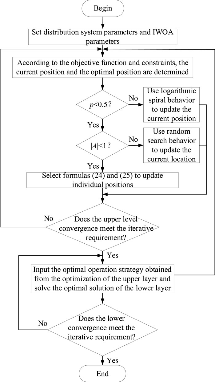
This article adopts an IWOA to solve the upper- and lower-layer models, featuring faster convergence speed and good global search capability. The relationship between the upper and lower layers of the joint model is shown in Figure 10, and the solving process is presented in Figure 11.

Figure 10

Figure 10. Double-layer model interaction.

Figure 11

Figure 11. The solution flow of two-layer programming.

5 Case study

5.1 Example parameters and settings

In this article, the model is verified and analyzed using the IEEE-33 node distribution system, and the example topology is shown in Figure 12. The scenario outputs of the system are shown in Figures 7–9.

Figure 12

Figure 12. Distribution system based on the IEEE-33 node distribution system.

The parameters of the IWOA algorithm are set as follows: the population size of both the upper and lower layers of the two-layer programming model is set to 200, and the maximum number of iterations is set to 200.

5.2 Model results analysis

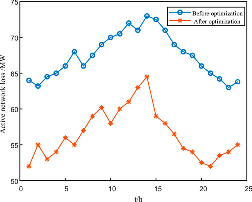
Based on the two-layer optimization model for the distribution network established in this article, the planning results for DGs and energy storage are shown in Table 2. The comparison results of system network losses and voltage magnitude before and after optimization are shown in Figures 13, 14.

Table 2

Table 2. DG and energy storage planning results.

Figure 13

Figure 13. Comparison of system network losses before and after optimization.

Figure 14

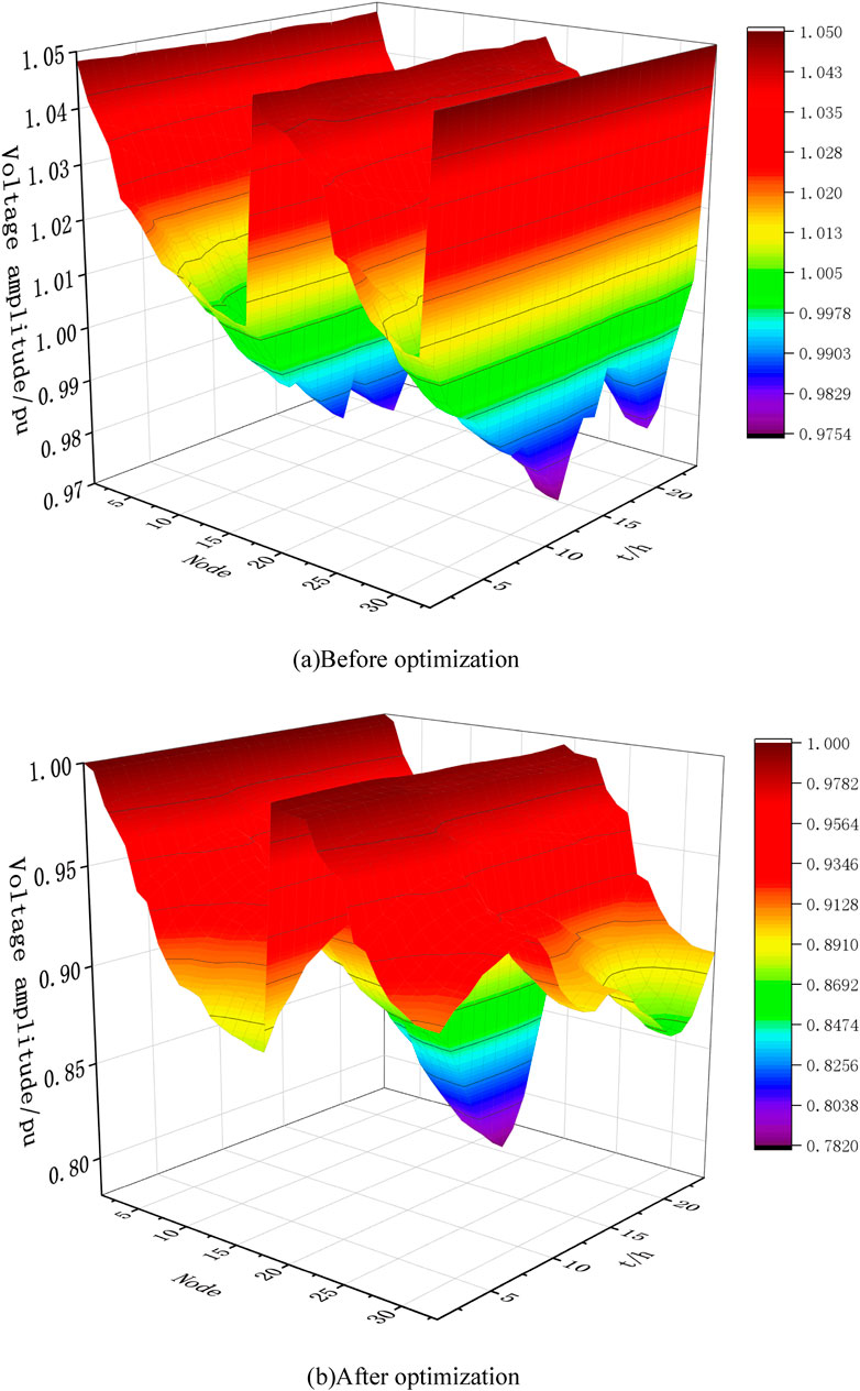
Figure 14. Comparison of voltage magnitudes at various moments in the system before and after optimization. (A) Before optimization . (B) After optimization.

It is observed that the active power grid loss of the system significantly decreases after optimization. Before the introduction of distributed power sources and energy storage systems, the system’s average grid loss over 24 h was 67.49 MW. After introducing distributed power sources and energy storage systems, the system’s average grid loss was 56.53 MW, with a system loss reduction rate of 16.1%. The results show that the reasonable location of DGs reduces the long-distance transmission loss, and the BESS peak shaving and valley filling improve the time series power flow distribution, suppress the power fluctuation, and significantly reduce the line loss.

It can be seen that before optimization, some node voltages exceeded the system’s safe range, but after optimization, the voltage amplitude has been overall improved and maintained within a reasonable range. This is because the BESSs smooth out the voltage fluctuations through dynamic charge and discharge, absorb excess power during the day to prevent over-voltage, and compensate for the power gap at night to support voltage stabilization.

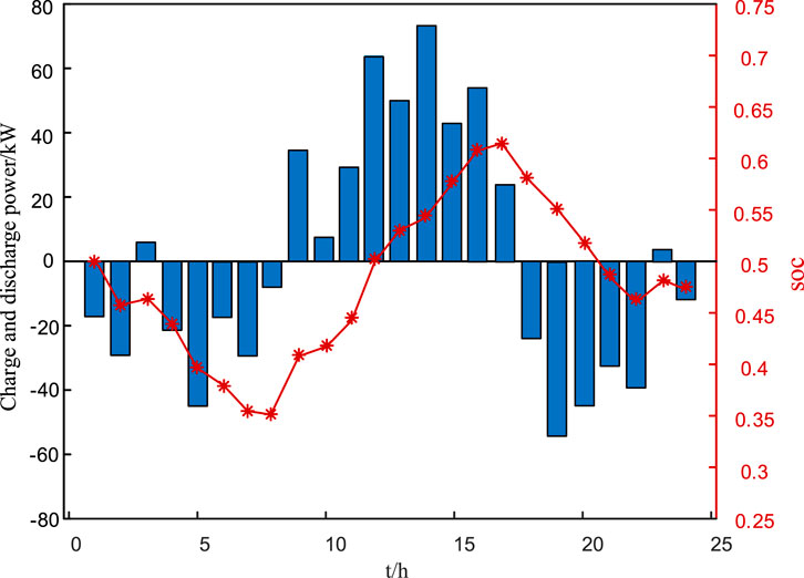
To further verify the feasibility and superiority of the IWOA proposed in this article, the initial SOC of BESSs is set to 50% in the simulation. The charging and discharging strategies of the optimized energy storage system at each moment within 24 h, as well as the changes in the state of the charge curve, are shown in Figure 15.

Figure 15

Figure 15. Energy storage charge/discharge power vs. charge state variation curve.

It can be seen that during the day, the energy storage system absorbs excess energy from the power grid, and the charge state curve of the storage during this period shows an upward trend. At night, the energy storage system discharges to the grid, alleviating grid pressure and resulting in a downward trend in the charge state curve. In addition, the charging and discharging power of the energy storage system is basically balanced, effectively maintaining the charge state of the storage device within the specified range. Based on the optimized scheduling strategy, it can be seen that BESSs not only provide the function of load peak and valley reduction but also optimize the power flow and frequency support by dynamically responding to wind and solar fluctuations.

5.3 Scenario comparison analysis

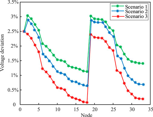
Three different scenarios are set for comparative analysis to verify the effectiveness and superiority of the model proposed in this article. In Scenario 1, only DGs are added to the IEEE-33 node distribution system without connecting to BESSs. In Scenario 2, both DGs and BESSs are added, and no optimization algorithms are used. In Scenario 3, both DGs and BESSs are added, and the IWOA is used. The planning schemes and costs for each scenario are shown in Table 3, 4, respectively. At that point, the node active power loss and node voltage deviation under the three scenarios are compared and analyzed, as shown in Figures 16, 17.

Table 3

Table 3. Planning scheme of each scenario.

Table 4

Table 4. Planning cost of each scenario.

Figure 16

Figure 16. The active power network loss curve of each node.

Figure 17

Figure 17. Voltage deviation curves of each node.

It is observed that the active power grid loss and voltage deviation in Scenario 3 are lower than those in Scenario 1 and Scenario 2. When comparing Scenario 1 with Scenario 2, it can be observed that with the addition of energy storage, the overall active power loss decreased by 764 kW, and the active power loss rate decreased by 12.3%. The overall voltage deviation decreased by 8.9%. When comparing Scenario 2 with Scenario 3, the overall active power loss based on the IWOA is decreased by 1.14 MW, and the active power loss rate decreased by 17.6%. The overall voltage deviation decreased by 23.8%. This is due to the collaborative optimization of DGs and BESSs; DGs with reasonable site selection can effectively reduce the transmission loss, and the dynamic scheduling of BESSs enhances the system voltage support capacity and operation flexibility so as to achieve the dual optimization of network loss and voltage. The IWOA optimization algorithm further improves the global optimality of site selection and scheduling and enhances the adaptability of the system to the randomness of wind and solar output. In the integrated wind–solar–storage mode, the energy storage system effectively absorbs the fluctuation of wind and solar, which not only optimizes the power flow distribution but also significantly improves the voltage quality, providing key support for the improvement of the operation performance and economy of the distribution network. The above comparisons demonstrate that the optimization model proposed in this article has a good effect on the active power loss and voltage control of the system.

5.4 Analysis of algorithm improvement results

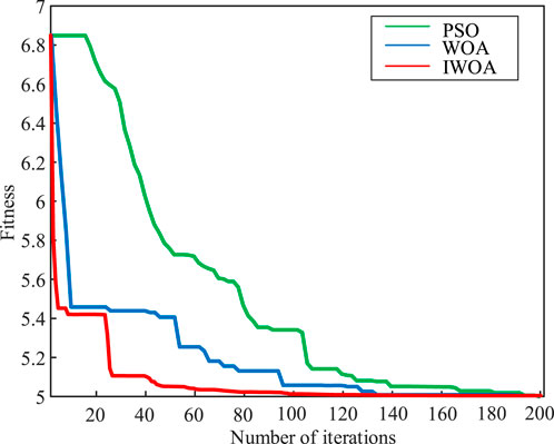
Figure 18 shows the convergence curves of the Particle Swarm Optimization algorithm (PSO), WOA, and IWOA when solving the two-layer optimal configuration model. As can be seen from the figure, the improved IWOA shows higher solution accuracy and faster convergence speed than the traditional PSO and WOA algorithms. In the first 20 iterations, the fitness value of IWOA decreases rapidly and approaches the optimal solution, showing obvious convergence advantages, while the PSO and WOA decrease rates are slower, and the final convergence effects are not as good as IWOA.

Figure 18

Figure 18. Comparative algorithm convergence curves.

By introducing nonlinear control parameters $l$ and optimizing the spiral update strategy, the improved IWOA improves the balance between local development and global exploration. It greatly improves the global optimal search ability and avoids the phenomenon of premature convergence, so the IWOA is better than the other two algorithms in terms of solution accuracy and convergence. This shows that IWOA has more efficient performance and better solution quality when solving the two-layer optimal configuration problem proposed in this article.

6 Conclusion

In this article, generative adversarial networks are first used to effectively learn the complex probability distribution of historical data of a high proportion of new energy generation, and new data samples with similar characteristics are generated. Then, a two-layer optimization model of the distribution network based on the IWOA and combining DGs and BESSs is proposed that addresses the high randomness introduced into the distribution network by the integration of a high proportion of renewable energy sources and the issues of high complexity, low efficiency, and susceptibility to local optimum traps in line loss calculation methods of traditional distribution networks. The results are as follows.

(1) Considering the high randomness and uncertainty introduced into the distribution network by the integration of a high proportion of renewable energy sources, a scenario generation method based on an improved GAN is proposed. This approach addresses the issues of the cumbersome modeling process, significant errors arising from parameter fitting, and poor quality of generated scenarios in traditional multi-scenario analysis methods.

(2) After adopting the two-layer optimal configuration model, the network loss of the distribution network system is reduced by 31.9%, and the voltage amplitude is improved as a whole and maintained within a reasonable range. It shows that the model can effectively improve the network loss and voltage of the distribution network with DGs and BESSs, which is beneficial to the safe and stable operation of the distribution network.

(3) Three different scenarios are set for comparative analysis to verify the effectiveness and superiority of the model proposed in this article.

Data availability statement

The original contributions presented in the study are included in the article/supplementary material; further inquiries can be directed to the corresponding author.

Author contributions

XM: writing–review and editing, methodology, supervision, and validation. XD: writing–review and editing, investigation, and software. HX: writing–review and editing, methodology, supervision, and validation. YL: writing–review and editing, data curation, and methodology. RX: writing–original draft, methodology, software, and validation. KW: writing–review and editing, software, supervision, and validation. JC: writing–review and editing, investigation, software, and validation. JW: writing–review and editing, investigation, methodology, and software.

Funding

The author(s) declare that no financial support was received for the research, authorship, and/or publication of this article. This work was supported by the Project of the Electric Power Research Institute of State Grid Gansu Electric Power Company (52272223000Z) and Lanzhou Talent Innovation and Entrepreneurship (2022-RC-17).

Conflict of interest

Authors XM, YL, XD, RX, and KW were employed by the Electric Power Research Institute of State Grid Gansu Electric Power Company.

Author HX was employed by the State Grid Gansu Electric Power Company.

The remaining authors declare that the research was conducted in the absence of any commercial or financial relationships that could be construed as a potential conflict of interest.

The authors declare that this study received funding from State Grid Gansu Electric Power Company. The funder had the following involvement in the study: the study design, data collection and analysis, decision to publish, or preparation of the manuscript.

Generative AI statement

The author(s) declare that no Generative AI was used in the creation of this manuscript.

Publisher’s note

All claims expressed in this article are solely those of the authors and do not necessarily represent those of their affiliated organizations, or those of the publisher, the editors and the reviewers. Any product that may be evaluated in this article, or claim that may be made by its manufacturer, is not guaranteed or endorsed by the publisher.

References

Cai, C., Li, Y., He, Y., and Guo, L. (2023). Two-tier coordinated optimal scheduling of wind/PV/hydropower and storage systems based on generative adversarial network scene generation. Front. Energy Res. 11. doi:10.3389/fenrg.2023.1266079

CrossRef Full Text | Google Scholar

Chen, Z., Jia, R., Wang, S., Nan, H., Zhao, L., Zhang, X., et al. (2024). Two-layer optimal scheduling of distribution network-multi-microgrids based on master-slave game. Front. Energy Res. 12. doi:10.3389/fenrg.2024.1450731

CrossRef Full Text | Google Scholar

Dai, R., Zhang, X., and Zou, H. (2024). Two-stage distributed robust optimal allocation of integrated energy systems under carbon trading mechanism. Processes 12 (6), 1044. doi:10.3390/pr12061044

CrossRef Full Text | Google Scholar

Deb, K., and Jain, H. (2014). An evolutionary many-objective optimization algorithm using reference-point-based nondominated sorting approach, Part I: solving problems with box constraints. IEEE Trans. Evol. Comput. 18(4), 577–601. doi:10.1109/tevc.2013.2281535

CrossRef Full Text | Google Scholar

Feng, Y., Long, L., and Qian, J. (2023). Monthly probability theoretical line loss calculation method of low voltage distribution network based on simultaneous power and electricity. IEEE Access 11, 145792–145800. doi:10.1109/access.2023.3344576

CrossRef Full Text | Google Scholar

Hu, W., Guo, Q., Wang, W., and Song, S. (2022). Loss reduction strategy and evaluation system based on reasonable line loss interval of transformer area. Appl. Energy. 306, 118123–123. doi:10.1016/j.apenergy.2021.118123

CrossRef Full Text | Google Scholar

Huo, X. Z., Liu, Y. Q., and Zhou, X. H. (2023). Research on distribution network line loss prediction based on improved grey relational analysis and stacking algorithm. J. North China Electr. Power Univ., 1–8.

Google Scholar

Li, J., Hang, J. M., and Zhu, J. Q. (2017). Line loss calculation for distribution network based on state characterization. Power Syst. Prot. contr. 45 (10), 55–61. doi:10.7667/PSPC160745

CrossRef Full Text | Google Scholar

Liao, J., Lin, J., and Wu, G. (2024). Two-layer optimization configuration method for distributed photovoltaic and energy storage systems based on IDEC-K clustering. Energy Rep. 11, 5172–5188. doi:10.1016/j.egyr.2024.04.047

CrossRef Full Text | Google Scholar

Liu, J. Y., Lyu, L., and Gao, H. J. (2022). Planning of active distribution network considering characteristics of distributed generator and electric vehicle. Autom. Electr. Power Syst. 44 (12), 41–48. doi:10.7500/AEPS20190826001

CrossRef Full Text | Google Scholar

Liu, Y., Wang, Y., and Yang, Q. (2023). Spatio-temporal generative adversarial network based power distribution network state estimation with multiple time-scale measurements. IEEE Trans. Ind. Inf. 19(9), 9790–9797. doi:10.1109/tii.2023.3234624

CrossRef Full Text | Google Scholar

Ma, X. P., Jia, R., and Liang, C. (2022). Review of researches on loss reduction in context of high penetration of renewable power generation. Power Syst. Technol. 46 (11), 4305–4315.

Google Scholar

Pegado, R., Naupari, Z., Molina, Y., and Castillo, C. (2019). Radial distribution network reconfiguration for power losses reduction based on improved selective BPSO. Electr. Power Syst. Res. 169, 206–213. doi:10.1016/j.epsr.2018.12.030

CrossRef Full Text | Google Scholar

Shahraki, M. H., Zamani, H., and Varzaneh, Z. A. (2023). A systematic review of the whale optimization algorithm: theoretical foundation, improvements, and hybridizations. Arch. Comput. Methods Eng. 30 (7), 4113–4159. doi:10.1007/s11831-023-09928-7

CrossRef Full Text | Google Scholar

Shao, Z., Zhang, C., and Chen, F. (2019). Generative adversarial networks and their applications in power systems. Proc. CSEE, 43(3), 987–1004.

Google Scholar

Sultana, B., M. Mustafa, W., Sultana, U., and Bhatti, A. R. (2016). Review on reliability improvement and power loss reduction in distribution system via network reconfiguration. Renew. Sustain. Energy Rev. 66 (4), 297–310. doi:10.1016/j.rser.2016.08.011

CrossRef Full Text | Google Scholar

Wang, H. j., Cao, W. J., and Zhang, Y. (2023a). Online calculation of distribution network line loss based on RF and KRR. South. Power Syst. Technol. 17 (08), 104–112.

Google Scholar

Wang, S. J., Xia, G. F., and Chen, G. G. (2021). A distributed generation planning method for distribution network based on k-medoid clustering. Power Syst. Clean. Energy. 37 (02), 132–138.

Google Scholar

Wang, S. X., Qi, L., and Ji, X. Q. (2017). A fast sensitivity method for determining line loss and node voltages in active distribution network. IEEE Trans. Power Syst. 33 (1), 1148–1150. doi:10.1109/TPWRS.2017.2735898

CrossRef Full Text | Google Scholar

Wang, Y. F., Liao, R. H., and Liang, E. H. (2023b). Improved whale optimization algorithm based on siege mechanism. Contr. Decis. 38 (10), 2773–2782. doi:10.13195/j.kzyjc.2022.0425

CrossRef Full Text | Google Scholar

Wu, H., Yuan, Y., and Ma, K. (2020). A novel probabilistic method for energy loss estimation using minimal line current information. IEEE Trans. Power Syst. 35 (6), 4928–4931. doi:10.1109/tpwrs.2020.3020719

CrossRef Full Text | Google Scholar

Wu, L. Z., Qin, W. B., and Zhao, Y. F. (2023). Distribution network line loss prediction method based on TASSA-Mg LSTM. Proc. CSU-EPSA., 1–10. doi:10.19635/j.cnki.csu-epsa.001217

CrossRef Full Text | Google Scholar

Xie, L., Li, H. W., and Yuan, Y. (2021). Calculation of line loss in transformer district based on K-Means clustering algorithm and improved MRVM. J. Electr. Eng. 16 (01), 62–69. doi:10.11985/2021.01.009

CrossRef Full Text | Google Scholar

Xun, X., Lirong, X., and Lin, Y. (2022). Active power two-layer optimization model of wind farm based on nonparametric kernel density estimation. Automation Electr. Power Syst., 46(02):43–55.

Google Scholar

Yao, M., Zhu, Y., Li, J., Wei, H., and He, P. (2019). Research on predicting line loss rate in low voltage distribution network based on gradient boosting decision tree. Energies 12 (13), 2522–22. doi:10.3390/en12132522

CrossRef Full Text | Google Scholar

Yi, D., Yu, M., Wang, Q., Tian, H., Wang, L., Yan, Y., et al. (2024). Method for wind–solar–load extreme scenario generation based on an improved InfoGAN. Appl. Sci., 14(20), 9163. doi:10.3390/app14209163

CrossRef Full Text | Google Scholar

Yuan, R., Wang, B., Sun, Y., Song, X., and Watada, J. (2023). Conditional style-based generative adversarial networks for renewable scenario generation. IEEE Trans. Power Syst. 38 (2), 1281–1296. doi:10.1109/tpwrs.2022.3170992

CrossRef Full Text | Google Scholar

Yuanze, M., Liu, C., Yang, J., Zhang, H., and Wu, Q. (2021). Low-carbon generation expansion planning considering uncertainty of renewable energy at multi-time scales. Glob. Energy Interconnect., 4(3), 261–272. doi:10.1016/j.gloei.2021.07.005

CrossRef Full Text | Google Scholar

Zhang, S. X., and Shao, H. Z. (2017). Optimization research of distribution network considering distributed generation. Electr. Power. 50 (03), 147–153.

Google Scholar

Zhang, X., Li, D., and Fu, X. (2024). A novel wasserstein generative adversarial network for stochastic wind power output scenario generation. IET Renew. Power Gener. 18, 3731–3742. doi:10.1049/rpg2.12932

CrossRef Full Text | Google Scholar

Zhang, Y., Xu, Y., and Zhang, Y. (2021). Prediction model of line loss rate in the station area based on the multivariate linear regression integrated with a new K-means clustering algorithm. J. Electr. Power Sci. Technol. 36 (5), 179–186. doi:10.19781/j.issn.1673-9140.2021.05.022

CrossRef Full Text | Google Scholar

Zhang, Z., Lei, D., Li, J., and Xu, Y. (2022). Source-network-load-storage bi-level collaborative planning model of active distribution network with SOP based on adaptive e-dominating multi-objective particle swarm optimization algorithm. Power Syst. Technol. 46 (6), 2199–2209. doi:10.13335/j.1000-3673.pst.2021.1098

CrossRef Full Text | Google Scholar