An optimized method for short-term load forecasting based on feature fusion and ConvLSTM-3D neural network

As renewable energy continues to penetrate modern power systems, accurate short-term load forecasting is crucial for optimizing power generation resource allocation and reducing operational costs. Traditional forecasting methods often overlook key factors such as holiday load variations and differences in user electricity consumption behavior, resulting in reduced accuracy. To address this, we propose an optimized short-term load forecasting method based on time and weather-fused features using a ConvLSTM-3D neural network. The Prophet algorithm is first employed to decompose historical electricity load data, extracting feature components related to time variables. Simultaneously, the SHAP algorithm filters weather variables to identify highly correlated weather features. A time attention mechanism is then applied to fuse these features based on their correlation weights, enhancing their impact within the time series. Finally, the ConvLSTM-3D model is trained on the fused features to generate short-term load forecasts. A case study using real-world data validates the proposed method, demonstrating significant improvements in forecasting accuracy.

1 Introduction

Accurate electricity load forecasting, particularly short-term electricity forecasting (STLF), is a vital component of the safe operation of contemporary power systems and provides significant guidance for energy dispatch (Yang et al., 2022; Si et al., 2023). However, on the electricity load demand side, with technological advancements and changing climate conditions, the usage of new electric equipment such as electric vehicles (EVs), air conditioners, and smart home devices has increased sharply (Ahmad et al., 2022; Pijarski and Belowski, 2024). This surge in usage introduces greater uncertainty into electrical load forecasts. Furthermore, electricity load is not only affected by weather conditions such as temperature, humidity, and precipitation, but also influenced by residential consumption habits at different times, such as holidays and weekly seasonality (Yang et al., 2022). Accurate load forecasting is an effective method for managing energy consumption, facilitating the production of a reliable electricity trade market, and ensuring the frequency safety and stability of the new power system (Ahmad et al., 2022). More importantly, as the complexity of power systems increases, the need for precise forecasts becomes crucial (Abdolrasol et al., 2021). Therefore, it is imperative to improve load forecasting accuracy, prompting more researchers to engage in this area of study.

Early load forecasting methods were primarily based on statistical models, such as ARMA, ARIMA, and HAR. While these statistical models have fewer parameters and offer relatively high computational efficiency, they struggle to process nonlinear data, making it difficult to meet the current demands of variable power load forecasting (Ahmad et al., 2022). With the advancement of artificial intelligence and the increased computing power of modern systems, load forecasting methods based on artificial neural networks (ANNs) have gained widespread use (Abdolrasol et al., 2021). Mainstream ANNs used for power system load forecasting include models like SVR, GRU, LSTM, and BP neural networks. Compared to statistical methods, ANN-based models can effectively capture the temporal characteristics of nonlinear data, leading to more accurate predictions (Liu et al., 2018; Wang et al., 2012). However, the performance of these models is highly sensitive to the choice of structural parameters and the quality of the training data. This can result in issues such as overfitting or underfitting. Additionally, these models require data sets with high integrity and appropriate sampling rates (Wazirali et al., 2023). The large variations in load data collected across different devices and regions also place high demands on the robustness of prediction models. Consequently, despite their advantages, ANN-based models may struggle to meet the evolving needs of today’s load forecasting (Ding et al., 2015).

With the continued advancement of artificial intelligence, load forecasting methods based on deep learning models have been widely adopted in recent years. Compared to traditional artificial neural networks, deep learning models feature more hidden layers and possess powerful feature extraction capabilities. For example, reference (Dong et al., 2024) proposes a multi-node load forecasting method for power systems using a deep learning multi-time scale convolutional model integrated with a Transformer model. This fused model excels at capturing the temporal and spatial characteristics of data, resulting in notable improvements in multi-node power system load forecasting. Similarly, reference (Zhuang et al., 2023) leverages a graph attention network and a one-dimensional convolutional neural network to extract the temporal and spatial characteristics of regional loads, allowing the model to better explore the spatial dependencies of regional loads and provide richer feature variables for prediction. Reference (Huang et al., 2023) introduces a deep learning model combining Spearman correlation, GCN, and GRU. The Spearman correlation coefficient quantifies the relationship between loads at different nodes, while the GCN captures spatial correlations, and GRU mines the temporal relationships within the data. A well-designed deep learning model can fully explore the latent features in data, playing a critical role in enhancing prediction accuracy. Given the complexity of feature variables involved in short-term load forecasting—particularly for bus loads—the model employed in this paper must have strong feature extraction capabilities.

In short-term load forecasting, the selection of training features is crucial to achieving accurate predictions. Current time-series-based prediction methods typically utilize historical data, meteorological data, and calendar data for forecasting (Liu et al., 2020). However, the influence and weight of different meteorological and calendar data on load forecasting vary significantly. Using these data directly as features can result in suboptimal predictions, and an excessive number of features can introduce redundancy. Furthermore, calendar data generally only include broad information such as holidays, weekdays, and workdays, which fails to capture the specific effects of various time-related factors on load (Dahl et al., 2018). To address these limitations, reference (Yang et al., 2023) employs multidimensional time domain features as model inputs for forecasting. First, a load feature decomposition model based on a periodic trend decomposition algorithm is constructed to obtain feature components that reflect the load’s trend, periodicity, and randomness. Similarly, reference (Zhan et al., 2022) decomposes load data into a series of sub-modal data with different central frequencies through variational mode decomposition, and clusters these sub-modal data to extract feature quantities of different frequency centers. Reference (Chen C. et al., 2024) introduces derivative terms, using the difference between vector values as supplementary features to capture load change characteristics across different time periods. While these methods have achieved certain improvements by optimizing feature selection, they do not comprehensively consider the influence weights of specific features, such as time and weather features. Thus, further optimization of feature processing is still needed to enhance the accuracy of short-term load forecasting.

Building on these approaches, this paper proposes a short-term load forecasting method that integrates time and weather fusion features with a ConvLSTM-3D neural network. First, the historical power load data is preprocessed to align with corresponding timestamps and labeled with relevant data such as holidays, years, seasons, months, weeks, workdays, and non-workdays. Next, the Prophet algorithm is employed to extract time feature components from the dataset, generating various feature quantities related to power load. Concurrently, the SHAP algorithm is utilized to filter weather variables, identifying the most strongly correlated weather feature components. Based on the correlation weights of these feature components, a time attention mechanism is applied to fuse the features, effectively combining the time and weather components while increasing their respective influence on the time series. Finally, the fused features are input into the ConvLSTM-3D model to train the system and produce future short-term power load forecasts.

2 Time-weather fusion features

2.1 Time component extraction using the prophet algorithm

Compared to ultra-short-term load forecasting, short-term power load forecasting operates on a relatively longer time scale. As a result, power load is influenced by various time-related factors, such as users’ power consumption habits, holiday patterns, and power demand across different periods. Additionally, the impact and significance of these time components on power consumption vary. Therefore, to enhance the accuracy of short-term power load forecasting, it is essential to incorporate diverse time components as key features in the prediction model.

The Prophet algorithm, developed by Facebook, is a time series forecasting tool designed to handle data with strong seasonality and is highly robust to missing data and sudden trend changes (Ceperic et al., 2013). Compared to traditional algorithms, Prophet offers simpler parameter tuning and allows users to adapt parameters to different scenarios. In this paper, the Prophet algorithm is employed to extract various time components from the original power load data, including trend components, holiday characteristics, weekly characteristics, and daily characteristics. The calculation expression for this process is shown in Equation 1.

$y\left(t\right)=g\left(t\right)+s\left(t\right)+v\left(t\right)+\epsilon \left(t\right)(1)$

where $y\left(t\right)$ represents the original power load, $g\left(t\right)$ represents the trend term, which represents the trend of the time series in the non-periodic aspect, $s\left(t\right)$ represents the periodic term; $v\left(t\right)$ is the holiday term, it represents the impact of the potential non-fixed periodic holidays in the time series on the predicted value, $\epsilon \left(t\right)$ represents the error term, which represents the fluctuation predicted by the model.

In the trend term, two important functions are employed: one based on logistic regression (non-linear growth) and the other based on piecewise linear functions (linear growth). The trend component base4d on logistic regression can be expressed as Equation 2.

$g\left(t\right)=\frac{C\left(t\right)}{1+\exp \left(-\left(k+a{\left(t\right)}^T\delta \right)\cdot \left(t-\left(m+a{\left(t\right)}^T\gamma \right)\right)\right)}(2)$

where $C\left(t\right)$ represents the carrying capacity, which is a function that changes with time and limits the maximum value that can grow. $k$ represents the growth rate, and $m$ represents the offset. In addition, the trend term expression based on the piecewise linear function is in Equation 3.

$g\left(t\right)=\left(k+\mathit{a}{\left(t\right)}^T\mathit{\delta }\right)\cdot t+\left(m+\mathit{a}{\left(t\right)}^T\mathit{\gamma }\right)(3)$

where $k$ represents the growth rate, $\delta$ represents the change in the growth rate, and $m$ represents the offset. Since the short-term forecast data of the load belongs to nonlinear growth, the growth term is represented by logistic regression. For the periodic term, the Prophet algorithm uses Fourier series to represent it, and its expression is Equation 4.

$s\left(t\right)={\displaystyle \sum _{\gamma =1}^N}\left(a_{\gamma }\cos \left(\frac{2\pi \gamma t}{P}\right)+b_{\gamma }\sin \left(\frac{2\pi \gamma t}{P}\right)\right)(4)$

$\rho =\left\{a_1,b_1,a_2,b_2,\cdots ,a_N,b_N\right\}(5)$

In the formula, $P$ is the period in days; $\rho$ is the set of smoothing coefficients $a_{\gamma }$ and $b_{\gamma }$, which satisfies the normal distribution; N is the number of smoothing coefficients $a_{\gamma }$ or $b_{\gamma }$, $\gamma$ is the sequence number of the smoothing coefficient. The holiday term can be represented as Equation 6.

$v\left(t\right)=Z\left(t\right)\kappa (6)$

where $Z\left(t\right)$ is the regression matrix, and $\kappa$ is the prior change parameter corresponding to holidays.

On the other hand, the hyperparameters of the Prophet model include the changepoint prior scale (CPS), seasonality prior scale (SPS), and holiday prior scale (HPS). The CPS dictates the model’s sensitivity to trend shifts, SPS regulates the strength of the seasonal components, and HPS governs the magnitude of holiday effects. The training and optimization process can be summarized as follows.

Algorithm 1.The training and optimization process of Prophet algorithm.

Define parameter ranges

 CPS from 0.001 to 0.5

 SPS from 0.01 to 10

 HPS from 0.01 to 10

Initialize:

 best_params as empty dictionary

 best_perf as infinity

For each value in CPS

 For each value in SPS

  For each value in PHS

   Set model parameters (cps, sps, hps)

   Fit model on training data

   Evaluate model on validation data using RMSE

   If current RMSE < best_performance

    Update best_performance to current RMSE

    Update best_parameters to (CPS, SPS, HPS)

Output best_params and best_perf

2.2 Feature selection using SHAP algorithm

Different feature quantities have varying influence weights on the load. To enhance the interpretability of these feature components within the prediction model, this paper employs the SHAP (Shapley Additive Explanations) model to explain the contribution of each feature (Chen W. et al., 2024). SHAP is rooted in game theory and not only measures feature contributions in individual predictions but also aggregates the overall explanation of the model for local results. By calculating the Shapley value for each feature, SHAP provides the average contribution of each feature to the model’s predictions. The larger the SHAP value, the greater the influence of that feature on the model. Based on these values, features can be ranked, allowing us to identify which ones have the most significant impact on the prediction. For a load model, it can be characterized as Equation 7.

$\widehat{f}\left(x\right)=\left({\beta }_0,{\beta }_1{x}_1,\dots ,{\beta }_p{x}_p\right)(7)$

The influence of feature $x_p$ on the output result is related to its corresponding coefficient. Accordingly, the incremental contribution of feature $x_p$ is shown in Equation 8.

${\varphi }_j\left(\widehat{f}\right)={\beta }_j{x}_j-{\beta }_{j}E\left(X_j\right)(8)$

The Shapley value is calculated based on the average marginal contribution. For a given feature set S, the Shapley value for feature i is calculated using the following Equation 9:

${\varphi }_i\left(v\right)={\displaystyle \sum _{S\subseteq F|\left\{i\right\}}}\frac{\left|S\right|!\left(\left|F\right|-\left|S\right|-1\right)!}{\left|F\right|!}·\left(v\left(S\cup \left\{i\right\}\right)-v\left(S\right)\right)(9)$

where ${\varphi }_i\left(v\right)$ represents the SHAP value, $v\left(S\right)$ represents the predicted output when the model only uses the feature set S, $\left|S\right|$ is the number of features in the set S, $\left|F\right|$ is the total number of all features, and $v\left(S\cup \left\{i\right\}\right)-v\left(S\right)$ represents the marginal contribution when feature i is included compared to when it is not including.

2.3 Feature reconstruction based on attention mechanism

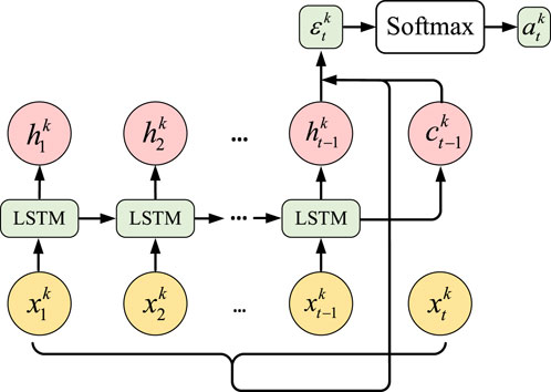
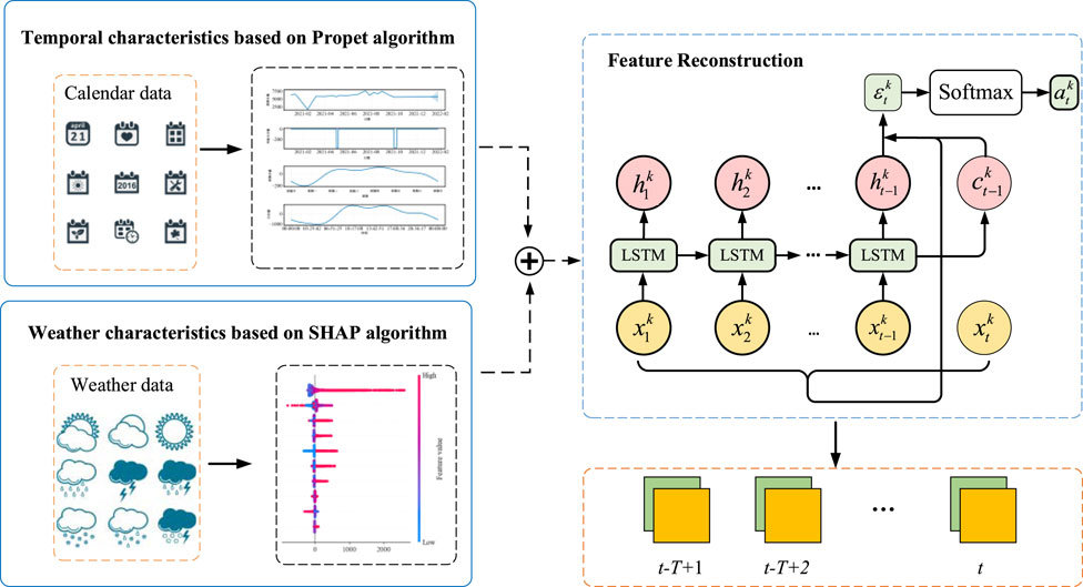
Since different feature components have varying influences on the load across different time periods, using the original feature data for prediction may reduce the influence weight of certain features over time. To address this, a time attention mechanism is applied to reconstruct the fused features. This paper employs an attention mechanism based on the LSTM computing unit to reconstruct the time series with different feature components, optimizing their impact on the time scale. The structure of this approach is shown in Figure 1.

Figure 1

Figure 1. Feature reconstruction model based on attention mechanism.

Taking fusion features $X^k=\left(x_1^k,x_2^k,\cdots ,x_L^k\right)\in R^L$ as an example, the similarity score between the hidden state and different attributes in LSTM is calculated based on the hidden state h_t-1 at time t-1. This score is then input into the Softmax function for normalization. The normalized similarity score is used to update the new feature sequence. After feature fusion, its expression can be represented as Equation 10.

$X^k=\left(x_1^k,x_2^k,\cdots ,x_L^k\right)\in R^L(10)$

where $X^k$ represents the fusion feature with k dimensions, and L represents the time length of the feature component. The input component after feature encoding is expressed as Equation 11.

${\epsilon }_t^k=V_{\epsilon }\tanh \left(W_{\epsilon c}{c}_{t-q}+W_{\epsilon h}{h}_{t-1}+b_i\right)(11)$

where $V_{\epsilon }$, $W_{\epsilon c}$,and $W_{\epsilon h}$ are parameters obtained based on LSTM structure training. The weight coefficients corresponding to different feature components can be expressed as Equation 12.

$a_t^k=\frac{\exp \left({\xi }_t^k\right)}{{\displaystyle \sum _{i=1}^n}\exp \left({\xi }_t^i\right)}(12)$

The feature components reconstructed through the attention mechanism can be represented as Equation 13.

${\stackrel{\sim }{x}}_t={\left(a_t^1{x}_t^1,a_t^2{x}_t^2,\cdots ,a_t^n{x}_t^n\right)}^{\mathrm{T}}(13)$

The combination of Prophet and SHAP uniquely addresses the limitations of traditional feature extraction and selection methods by leveraging Prophet’s robust decomposition of complex time series patterns into trend, seasonality, and holiday effects, while SHAP provides precise, interpretable feature importance. This synergy ensures enhanced interpretability, accurate feature attribution, and the ability to manage complex, nonlinear interactions, resulting in more robust and explainable forecasting models. Furthermore, the fusion features are optimized through the attention mechanism, effectively refining the impact of various feature components over different time scales. The process of constructing weather features based on time and weather fusion used in this paper is shown in Figure 2.

Figure 2

Figure 2. Feature reconstruction model based on attention mechanism.

3 Construction of short-term load forecasting model

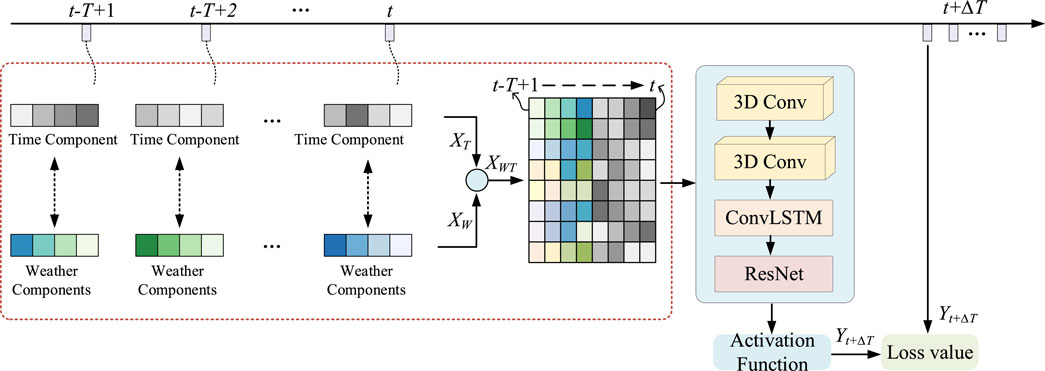
The fusion features constructed using the above method incorporate both time feature components and important weather feature components, with all components represented as time series. As a result, the fusion feature can be viewed as a three-dimensional feature with a time series dimension (Wang et al., 2021). To effectively model this, the ConvLSTM-3D deep learning network, which uses ConvLSTM as its basic structural unit, is adopted as the prediction model. The short-term load forecasting model and process developed in this paper are illustrated in Figure 4.

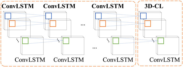
Compared to standard ConvLSTM, ConvLSTM-3D applies three-dimensional convolution operations in the input gate, forget gate, output gate, and cell state update, allowing for better handling of three-dimensional data (Moon et al., 2020; Mohammad et al., 2023). The input to each gate of the ConvLSTM unit contains three elements: memory information from the previous unit, output from the previous unit, and the input at the current time step. ConvLSTM consists of an input gate, forget gate, output gate, and memory unit. The model’s network structure is depicted in Figure 3A, while the schematic diagram of the internal structure of the unit is shown in Figure 3B (Guo et al., 2021; Alhussein et al., 2020).

Figure 3

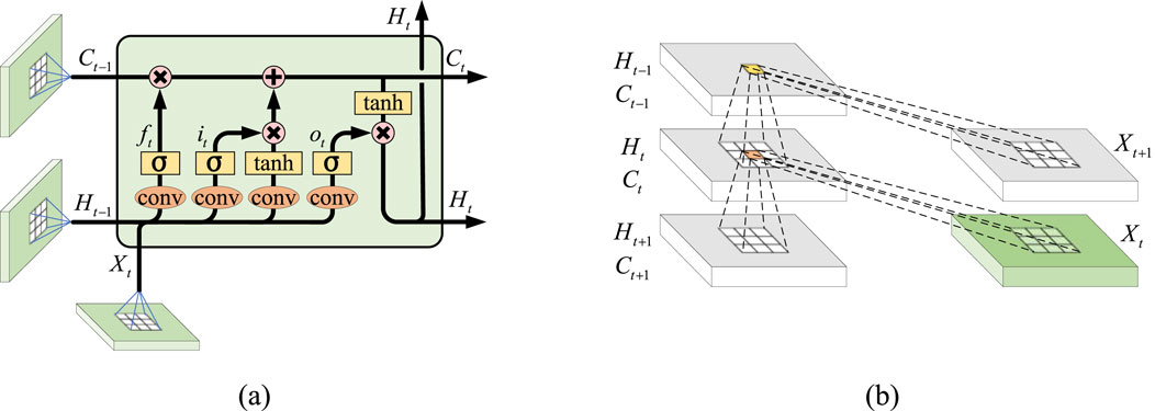
Figure 3. Forecasting model structure based on ConvLSTM. (A) ConvLSTM model structure diagram. (B) Internal structure of ConvLSTM unit.

3.1 Input gate

The input gate determines which parts of the current input should be updated in the memory cell. This process involves two steps: first, the sigmoid layer determines which information needs to be updated, and second, the tanh function generates candidate information. The structure of the input gate can be expressed as Equation 14.

$\left\{\begin{array}{l}{i}_t=\sigma \left(W_{xi}\ast {\chi }_t+W_{ht}\ast H_{t-1}+W_{ct}\ast C_{t-1}+b_i\right)\\ {\stackrel{\sim }{C}}_t=\tanh \left(W_{xc}\ast {\chi }_t+W_{hc}\ast H_{t-1}+b_c\right)\end{array}\right.(14)$

where $i_t$ and ${\stackrel{\sim }{C}}_t$ represent the output of the input gate and the backup information of the memory unit respectively, $x_t$ is the input data at the current time t, $C_{t-1}$ is the state information before the memory unit, $H_{t-1}$ is the output of the previous hidden layer unit of the ConvLSTM unit, $W$ and $b$ are the weight and bias of the input gate, respectively. $\sigma$ represents the sigmoid activation function, $\tanh$ represents the hyperbolic tangent function, and $\ast$ is the convolution operation.

3.2 Forget gate

The forget gate selectively discards unnecessary information from the memory unit from the previous time step. The forget gate can be expressed as Equation 15.

$f_t=\sigma \left(W_{xf}\ast {\chi }_t+W_{hf}\ast H_{t-1}+W_{cf}\ast C_{t-1}+b_f\right)(15)$

where $W_{xf}$ represents the weight of the information of the input layer flowing into the forget gate at this moment, $W_{hf}$ represents the weight of the final result of the previous hidden layer neural unit when the forget gate is input, $W_{cf}$ represents the weight of the memory unit state at the previous moment flowing into the forget gate, and $b_f$ represents the bias parameter when the forget gate is calculated.

3.3 Memory cell

The current memory unit state information $C_t$ is updated by describing the past long-term state and the current state. The process of updating the state information can be specifically expressed as Equation 16.

$C_t=f_t\ast C_{t-1}+i_t\ast {\stackrel{\sim }{C}}_t(16)$

3.4 Output gate

The output gate also consists of two parts. One part is the information input $O_t$,obtained by combining the short-term memory with the current input information (the output of the output gate at the current moment), and the other part $H_t$ is the final output after combining the long-term memory (the output of ConvLSTM at the current moment) which can be expressed as Equation 17.

$\left\{\begin{array}{l}{O}_t=\sigma \left(\begin{array}{l}{W}_{xo}\ast {\chi }_t+W_{ho}\ast H_{t-1}+\\ W_{co}\ast C_t+b_o\end{array}\right)\\ H_t=o_t\ast \tanh \left(C_t\right)\end{array}\right.(17)$

Compared with the traditional ConvLSTM model, this paper changes the loss function of the traditional ConvLSTM to make it more suitable for data features based on three-dimensional feature sequences. Its calculation is Equation 18 (Wang et al., 2021):

$SSIM\left(x,y\right)={\left[l\left(x,y\right)\right]}^a•{\left[c\left(x,y\right)\right]}^{\beta }•{\left[s\left(x,y\right)\right]}^{\gamma }(18)$

where $l\left(x,y\right)$, $c\left(x,y\right)$, and $s\left(x,y\right)$ represent brightness similarity index, contrast similarity index and structure similarity index respectively. The structure of the prediction model is shown in Figure 4. The short-term load forecasting process based on fusion features and ConvLSTM-3D model is shown in Figure 5.

Figure 4

Figure 4. Prediction model structure based on ConvLSTM.

Figure 5

Figure 5. Short-term load forecasting model structure based on fusion features and deep learning.

4 Case analysis

4.1 Data description and experimental simulation platform

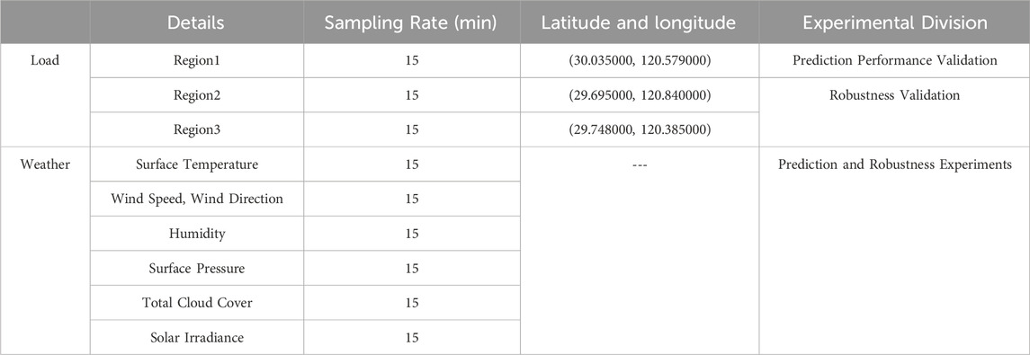
To verify the effectiveness of the fusion features and deep learning models proposed in this paper for short-term load forecasting, relevant measured data from a power grid company in a region of Zhejiang is used. The load data covers the power consumption of certain areas in the region from 2021 to 2023, with a sampling rate of one data point every 15 min. The weather data includes information such as surface temperature, wind speed, wind direction, and humidity from various areas within the region, also recorded at the same sampling rate. Key information about the load and meteorological data is summarized in Table 1.

Table 1

Table 1. Important information of the measured data set.

For verification, this paper uses the total social load data of a city in the region, with 80% of the data used as the training set and the remaining 20% for the test set. Additionally, to verify the robustness of the proposed method, load data from three other regions is used as supplementary verification, with corresponding meteorological data from these regions included. To compare and assess the computational efficiency of different experimental methods, all experiments are conducted on a unified experimental platform. The software platform is built using Python-based TensorFlow and PyTorch, while the hardware platform consists of an Intel Core i7-11700 (CPU) and an NVIDIA GeForce GTX 1660 Ti (GPU).

4.2 Evaluation metrics

In order to verify the prediction effect of the fusion features and deep learning model proposed in this paper on short-term power load, this paper uses the root mean square error (RMSE), mean absolute percentage error (MAPE) and determination coefficient (R square, R2) as the evaluation of the prediction model. Among them, RMSE is used to measure the distance between the actual value and the predicted value. MAPE is used to measure the percentage of the difference between the actual value and the actual value. R2 is used to measure the degree of explanation of the model for data changes. Its range is 0–1, and the larger the value, the better the model fits the sample (Wang et al., 2020; Bashir et al., 2022). The related calculation formulas are as Equations 19–21.

$\text{RMSE}=\sqrt{\frac{1}{n}{\displaystyle \sum _{i=1}^n}\left(y_i-{\widehat{y}}_i\right)}(19)$

$\text{MAPE}=\frac{1}{n}{\displaystyle \sum _{i=1}^n}\left|\frac{y_i-\widehat{y}}{y_i}\right|\ast 100\%(20)$

${\mathbf{R}}^2=1-\frac{{\displaystyle \sum _{i=1}^n}{\left(y_i-\widehat{y}\right)}^2}{{\displaystyle \sum _{i=1}^n}{\left(y_i-\overline{y}\right)}^2}(21)$

where $y_i$ is the actual observation value, ${\widehat{y}}_i$ is the predicted value, $\overline{y}$ is the average of the actual observation values, and $n$ represents the total number of observation points.

4.3 Forecasting results analysis

4.3.1 Temporal feature extraction results

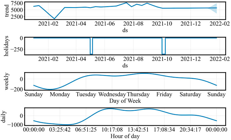
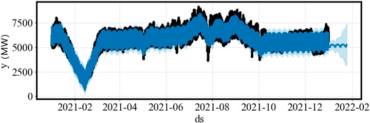
In the experiment, the Prophet algorithm was first applied to extract various time components of the region, with the results shown in Figure 6. And the error distribution of the Prophet algorithm for annual load forecasting is shown in Figure 7. As seen in the figure, the trend, holiday, week, and day components all have a significant impact on the overall power load in the region. Based on these observations, the trend, holiday, week, and day components were selected as the key time characteristics for the region.

Figure 6

Figure 6. Temporal feature components extracted using the Prophet algorithm.

Figure 7

Figure 7. Error distribution of the Prophet algorithm for annual load forecasting.

In addition, the SHAP algorithm was used to identify important weather feature components. SHAP quantifies the contribution of each feature to the forecast results, enabling the identification and explanation of weather features that significantly impact the model’s predictions (Yang et al., 2024). This method not only enhances the transparency of the model but also provides a scientific basis for further meteorological research and decision-making. The results of the SHAP analysis are shown in Figure 8.

Figure 8

Figure 8. Feature component contribution analysis based on SHAP values.

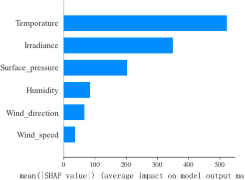
As seen in the figure, temperature changes have the greatest impact on power load among the weather characteristics. Significant fluctuations in output occur as the temperature increases or decreases. It is worth noting that total cloud cover has a much smaller impact on the output compared to the other six characteristics. Due to its minimal contribution, it is difficult to quantify using the SHAP algorithm and thus is not displayed in the figure. To more intuitively assess the importance of different meteorological components on the load, the average absolute SHAP value of each weather characteristic is used to rank their importance. The results of this ranking are shown in Figure 9.

Figure 9

Figure 9. Feature importance ranking based on mean absolute value SHAP.

The weather features were determined and selected based on the SHAP threshold value. In this study, a SHAP threshold of 200 was applied to distinguish the main contributors to feature importance from features exhibiting a rapid decline in importance. Consequently, the selected weather features in this research include temperature, irradiance, and surface pressure.

4.3.2 Forecasting result analysis

To verify the superiority of the method proposed in this paper, an ablation experiment was conducted to compare different feature sets and prediction models. For feature selection, the comparison includes a single time feature component, a single weather feature component, and the fusion feature component recommended in this study. Regarding the prediction models, a comparative analysis was performed between LSTM, CNN-LSTM, ConvLSTM, and ConvLSTM-3D (the model used in this paper). Additionally, to determine whether different time periods capture the characteristics of Chinese holidays, power load data from May 1st to May 3rd (during National Day) was compared with power load data from non-holiday periods in the region to evaluate the prediction performance. The 72-hour-ahead prediction comparison results are illustrated in Figure 10.

Figure 10

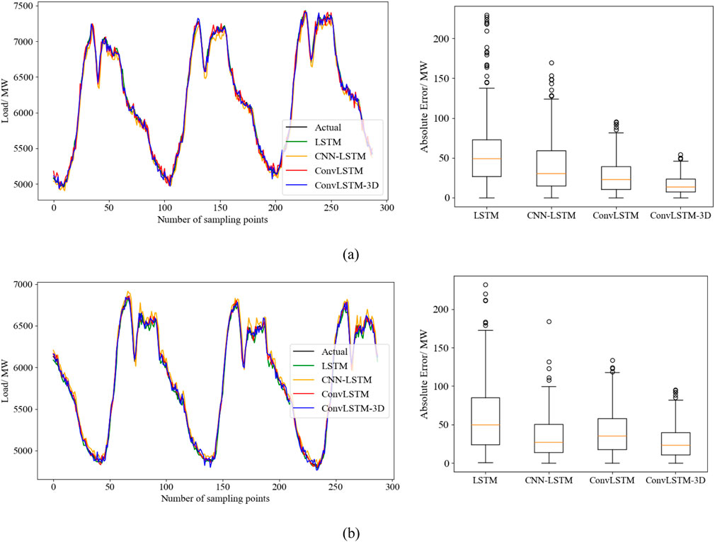
Figure 10. Comparison of forecasting results from different methods across different periods. (A) weekday load forecasting results. (B) holiday load forecasting results.

Figure 10A shows the load forecast curve from April 1 to 3 April 2023, representing the forecast results for non-holiday periods, while Figure 8B displays the load forecast curve from May 1 to 3 May 2023, representing the forecast results for holiday periods. By comparing and analyzing Figures 10A, B, it is evident that the power load in this area shows a noticeable upward trend during the holidays. Additionally, the load forecasting model proposed in this paper demonstrates superior performance in predicting power loads during both holiday and non-holiday periods.

To further validate the superior capabilities of the proposed forecasting models, supplementary experiments were conducted using a publicly available dataset from the Global Energy Forecasting Competition 2014 (GFC-2014), as referenced in research (Hong et al., 2016). The results of these additional forecasting experiments are presented in Figure 11.

Figure 11

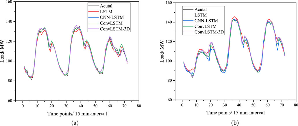
Figure 11. Comparison of forecasting results from different methods across different periods. (A) weekday load forecasting results. (B) holiday load forecasting results.

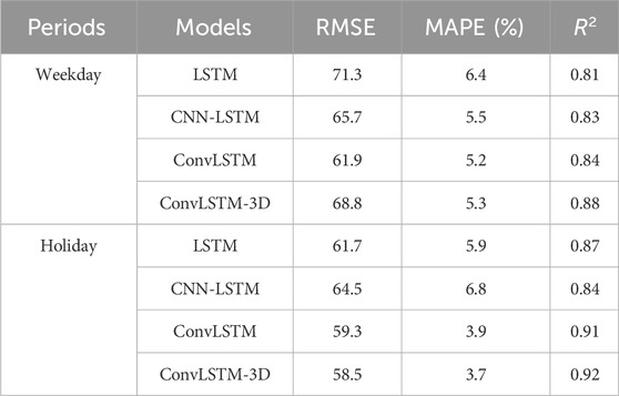
And the statistic of the forecasting performance of these comparison methods are summarized as Table 2.

Table 2

Table 2. Forecast results derived from the GFC-2014 model.

It can be observed that the method ConvLSTM-3D proposed in this research get the best performance across different period. This is because the superior capability capturing the spatial-temporal correlations of the fusion feature datasets. By comparison, the LSTM get the worst performance across the holidays as the load consumption behaviors cannot be captured by solely temporal models. And the CNN-LSTM forecast better than LSTM, because the CNN module can fill this gap. ConvLSTM better captures spatiotemporal features by directly modeling spatial and temporal dependencies through convolutional operations, while CNN-LSTM may lose information by separating spatial and temporal modeling. And ConvLSTM-3D enhances ConvLSTM by using 3D convolutions to capture spatiotemporal dependencies simultaneously, providing superior modeling of complex dynamics in tasks like video processing.

4.3.3 Ablation study based on feature analysis

To further validate the performance improvement of the short-term load forecasting method based on time-weather fusion features proposed in this paper, a comparative analysis was conducted. This analysis includes time features based on Prophet feature components, weather features derived from weather components, and fusion features combining both time and weather components. The experiment was performed using identical model parameters and training data for consistency.

The load forecast results were compared for non-holiday periods (April 1st to April 3rd) and holiday periods (May 1st to May 3rd), with the forecast result curves presented in Figure 12. Additionally, to further analyze the error distribution across different feature components, Figure 13 displays the average forecast error for the two forecast periods.

Figure 12

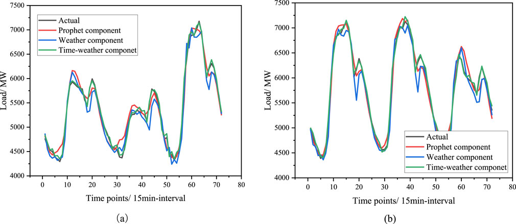
Figure 12. Forecasting results for different feature components and different time period. (A) Prediction result curves under different feature quantities during the non-holiday period (April 1 to April 3). (B) Prediction result curves under different feature quantities during the holiday period (May 1 to March 3).

Figure 13

Figure 13. 10 Average prediction error distribution under different feature components.

The results indicate that the prediction error distribution when using only Prophet feature components or only weather feature components is relatively divergent, whereas the prediction error with time-weather fusion features is more concentrated. This observation can be attributed to the inherent differences in power load characteristics among users during different time periods in short-term load forecasting. For instance, residents’ power consumption habits vary significantly between weekdays and holidays and demonstrate a correlation with weather conditions. Employing a model that relies solely on weather features or time features may lead to underfitting, ultimately resulting in lower prediction accuracy. The specific prediction statistical indicators are summarized in Table 3.

Table 3

Table 3. The experimental results of ablation based on feature analysis.

It is important to note that historical load data have been incorporated with the aforementioned features. The results demonstrated that the time-weather fusion features provided the most accurate forecasts across various periods, as this combination offers comprehensive insights into electrical consumption behaviors and the influence of weather conditions. In contrast, features relying solely on weather or social factors fail to capture a holistic representation of load consumption across different periods, neglecting variations in residents’ electricity usage patterns. The analysis of the experimental results clearly indicates that the proposed time-weather fusion feature significantly outperforms individual time-based or weather-based feature components.

4.3.4 Model robustness analysis

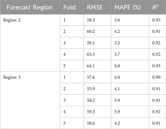
To verify the robustness and anti-interference capability of the model, 5-fold cross-validation was employed to evaluate the prediction results. Specifically, the dataset was divided into five distinct subsets. In each validation round, one of the subsets was designated as the validation set, while the remaining four subsets constituted the training set. The model was trained using the training set and subsequently evaluated using the validation set.

Performance was assessed using metrics such as mean square error and prediction accuracy, calculated after each validation round. This process yielded five sets of performance evaluation results, enabling analysis of the stability and generalization ability of the various prediction models. Since the robustness test assesses the performance of the model itself, independent of the training data, all comparison models utilized the same dataset. The validation was conducted using load data from regions 2 and 3, along with the corresponding meteorological data. The prediction results are presented in Table 4.

Table 4

Table 4. Five-fold cross validation test results.

The prediction accuracy of the short-term load forecasting method recommended in this paper matches the performance observed in the other two regions, demonstrating stability across different test and validation sets. This indicates that the method adopted in this paper is robust.

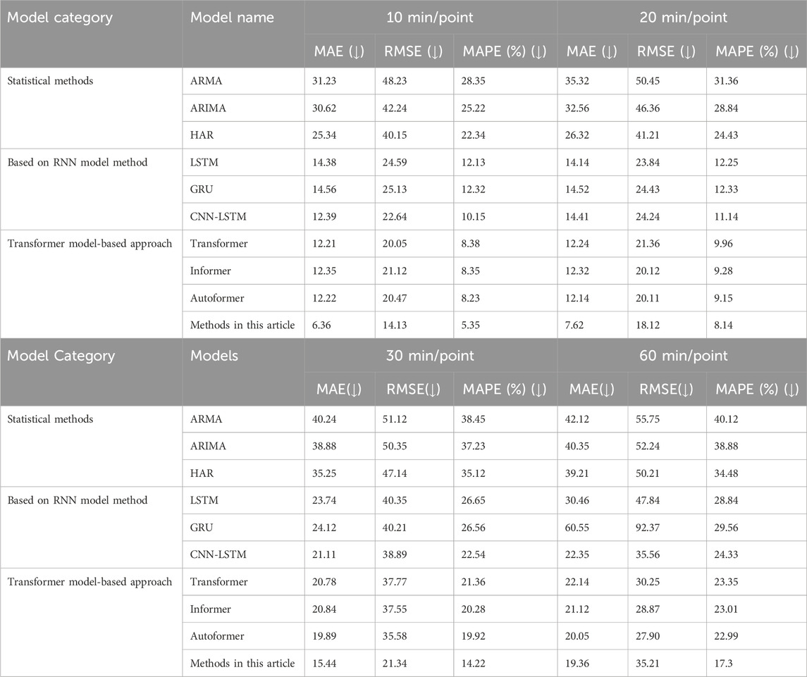
To thoroughly illustrate the improvements brought by the proposed method in short-term load forecasting, the experimental section compares and analyzes the prediction results of various models. Considering the differences between devices in different regions and the potential impacts of varying data sampling rates on new energy sources, this paper employs a downsampling method to enhance the model’s prediction performance across different sampling rates. The results are presented in Table 5. Additionally, post hoc Nemenyi tests are used to statistically analyze the prediction performance across multiple cross-experiments, with the statistical results depicted in Figure 14.

Table 5

Table 5. Performance comparison across different time intervals with various baseline models.

Figure 14

Figure 14. Post-hoc Nemenyi statistics of prediction results of different prediction models.

The horizontal axis in the chart represents the average ranking of each method, displayed from right to left, with a color gradient transitioning from black to blue. If the average ranking difference reaches the critical difference (CD), it is highlighted with a red line. For instance, the proposed model in this paper significantly outperforms the GRU, RNN, HAR, ARIMA, and SARIMA models. Similarly, the Autoformer model shows significantly better performance than the RNN, HAR, ARIMA, and SARIMA models. These statistical results underscore the superiority and robustness of the method proposed in this paper for short-term load forecasting.

5 Conclusion

In existing short-term load forecasting approaches, the accuracy of load predictions across regions (both temporally and spatially) is often inadequate. This is primarily due to the lack of consideration for factors such as holiday load variations and differences in user electricity consumption behavior, making it challenging for prediction models to extract correlations among complex feature variables. This paper proposes a short-term load forecasting framework that integrates time and weather fusion features with a ConvLSTM-3D deep learning model.

The framework consists of two key components: the construction of time-weather fusion features and the development of the ConvLSTM-3D prediction model. In the first stage, the Prophet algorithm is employed to extract various time feature components, followed by the selection of important weather feature components using the SHAP algorithm. Finally, based on the importance of the different feature components, the selected time and weather features are reconstructed using an attention mechanism.

In the second stage, the traditional ConvLSTM model is enhanced to create a ConvLSTM-3D prediction model that is suitable for the fused features, allowing for effective training and prediction with the constructed fusion features. By comparing the load prediction results across different algorithms, the proposed method demonstrates advancements in short-term load forecasting performance and the robustness of the model.

Data availability statement

The raw data supporting the conclusions of this article will be made available by the authors, without undue reservation.

Author contributions

XY: Methodology, Software, Validation, Writing–original draft. ShZ: Conceptualization, Formal Analysis, Investigation, Writing–review and editing. KL: Project administration, Supervision, Validation, Writing–review and editing. WC: Conceptualization, Data curation, Formal Analysis, Writing–review and editing. SiZ: Project administration, Resources, Visualization, Writing–review and editing. JC: Investigation, Validation, Visualization, Writing–review and editing.

Funding

The author(s) declare that financial support was received for the research, authorship, and/or publication of this article. The work is supported by State Grid Zhejiang Electric Power Co., LTD. Science and Technology project (B311SX23000C). The funder was not involved in the study design, collection, analysis, interpretation of data, the writing of this article, or the decision to submit it for publication.

Conflict of interest

Authors XY, ShZ, KL, WC, SiZ, and JC were employed by State Grid Zhejiang Electric Power Co., Ltd Shaoxing Power Supply Company.

Generative AI statement

The authors declare that no Generative AI was used in the creation of this manuscript.

Publisher’s note

All claims expressed in this article are solely those of the authors and do not necessarily represent those of their affiliated organizations, or those of the publisher, the editors and the reviewers. Any product that may be evaluated in this article, or claim that may be made by its manufacturer, is not guaranteed or endorsed by the publisher.

References

Abdolrasol, M. G. M., Hussain, S. M. S., Ustun, T. S., Sarker, M. R., Hannan, M. A., Mohamed, R., et al. (2021). Artificial neural networks based optimization techniques: a review. Electronics 10 (21), 2689. doi:10.3390/electronics10212689

CrossRef Full Text | Google Scholar

Ahmad, N., Ghadi, Y., Adnan, M., and Ali, M. (2022). Load forecasting techniques for power system: research challenges and survey. IEEE Access 10, 71054–71090. doi:10.1109/access.2022.3187839

CrossRef Full Text | Google Scholar

Alhussein, M., Aurangzeb, K., and Haider, S. I. (2020). Hybrid CNN-LSTM model for short-term individual household load forecasting. IEEE Access 8, 180544–180557. doi:10.1109/access.2020.3028281

CrossRef Full Text | Google Scholar

Bashir, T., Haoyong, C., Tahir, M. F., and Liqiang, Z. (2022). Short-term electricity load forecasting using hybrid prophet-LSTM model optimized by BPNN. Energy Rep. 8, 1678–1686. doi:10.1016/j.egyr.2021.12.067

CrossRef Full Text | Google Scholar

Ceperic, E., Ceperic, V., and Baric, A. (2013). A strategy for short-term load forecasting by support vector regression machines. IEEE Trans. Power Syst. 28 (4), 4356–4364. doi:10.1109/tpwrs.2013.2269803

CrossRef Full Text | Google Scholar

Chen, C., Li, S., Wen, M., and Yu, Z. (2024a). Ultra-short term wind power prediction based on quadratic variational mode decomposition and multi-model fusion of deep learning. Comput. Electr. Eng. 116, 109157. doi:10.1016/j.compeleceng.2024.109157

CrossRef Full Text | Google Scholar

Chen, W., Yang, K., Yu, Z., Shi, Y., and Chen, C. L. P. (2024b). A survey on imbalanced learning: latest research, applications and future directions. Artif. Intell. Rev. 57 (6), 137–151. doi:10.1007/s10462-024-10759-6

CrossRef Full Text | Google Scholar

Dahl, M., Brun, A., Kirsebom, O. S., and Andresen, G. B. (2018). Improving short-term heat load forecasts with calendar and holiday data. Energies 11 (7), 1678. doi:10.3390/en11071678

CrossRef Full Text | Google Scholar

Ding, N., Benoit, C., Foggia, G., Besanger, Y., and Wurtz, F. (2015). Neural network-based model design for short-term load forecast in distribution systems. IEEE Trans. power Syst. 31 (1), 72–81. doi:10.1109/tpwrs.2015.2390132

CrossRef Full Text | Google Scholar

Dong, Q., Huang, R., and Cui, C. (2024). Short-term electricity-load forecasting by deep learning: a comprehensive survey. arXiv Prepr. arXiv:2408.16202.

Google Scholar

Guo, W., Che, L., Shahidehpour, M., and Wan, X. (2021). Machine-Learning based methods in short-term load forecasting. Electr. J. 34 (1), 106884. doi:10.1016/j.tej.2020.106884

CrossRef Full Text | Google Scholar

Hong, T., Pinson, P., Fan, S., Zareipour, H., Troccoli, A., and Hyndman, R. J. (2016). Probabilistic energy forecasting: Global energy forecasting competition 2014 and beyond. Int. J. Forecast. 32 (3), 896–913. doi:10.1016/j.ijforecast.2016.02.001

CrossRef Full Text | Google Scholar

Huang, N., Wang, S., Wang, R., Cai, G., Liu, Y., and Dai, Q. (2023). Gated spatial-temporal graph neural network based short-term load forecasting for wide-area multiple buses. Int. J. Electr. Power and Energy Syst. 145, 108651. doi:10.1016/j.ijepes.2022.108651

CrossRef Full Text | Google Scholar

Liu, X., Zhang, Z., and Song, Z. (2020). A comparative study of the data-driven day-ahead hourly provincial load forecasting methods: from classical data mining to deep learning. Renew. Sustain. Energy Rev. 119, 109632. doi:10.1016/j.rser.2019.109632

CrossRef Full Text | Google Scholar

Liu, Y., Zhang, S., Chen, X., and Wang, J. (2018). Artificial combined model based on hybrid nonlinear neural network models and statistics linear models—research and application for wind speed forecasting. Sustainability 10 (12), 4601. doi:10.3390/su10124601

CrossRef Full Text | Google Scholar

Mohammad, F., Kang, D. K., Ahmed, M. A., and Kim, Y. C. (2023). Energy demand load forecasting for electric vehicle charging stations network based on convlstm and biconvlstm architectures. IEEE Access, 11: 67350–67369. doi:10.1109/access.2023.3274657

CrossRef Full Text | Google Scholar

Moon, J., Jung, S., Rew, J., Rho, S., and Hwang, E. (2020). Combination of short-term load forecasting models based on a stacking ensemble approach. Energy Build. 216, 109921. doi:10.1016/j.enbuild.2020.109921

CrossRef Full Text | Google Scholar

Pijarski, P., and Belowski, A. (2024). Application of methods based on artificial intelligence and optimisation in power engineering—introduction to the special issue. Energies 17 (2), 516. doi:10.3390/en17020516

CrossRef Full Text | Google Scholar

Si, F., Du, E., Zhang, N., Wang, Y., and Han, Y. (2023). China’s urban energy system transition towards carbon neutrality: challenges and experience of Beijing and Suzhou. Renew. Sustain. Energy Rev. 183, 113468. doi:10.1016/j.rser.2023.113468

CrossRef Full Text | Google Scholar

Wang, F., Mi, Z., Su, S., and Zhao, H. (2012). Short-term solar irradiance forecasting model based on artificial neural network using statistical feature parameters. Energies 5 (5), 1355–1370. doi:10.3390/en5051355

CrossRef Full Text | Google Scholar

Wang, Y., Chen, J., Chen, X., Zeng, X., Kong, Y., Sun, S., et al. (2020). Short-term load forecasting for industrial customers based on TCN-LightGBM. IEEE Trans. Power Syst. 36 (3), 1984–1997. doi:10.1109/tpwrs.2020.3028133

CrossRef Full Text | Google Scholar

Wang, Y., Sun, S., Chen, X., Zeng, X., Kong, Y., Chen, J., et al. (2021). Short-term load forecasting of industrial customers based on SVMD and XGBoost. Int. J. Electr. Power and Energy Syst. 129, 106830. doi:10.1016/j.ijepes.2021.106830

CrossRef Full Text | Google Scholar

Wazirali, R., Yaghoubi, E., Abujazar, M. S. S., Ahmad, R., and Vakili, A. H. (2023). State-of-the-art review on energy and load forecasting in microgrids using artificial neural networks, machine learning, and deep learning techniques. Electr. power Syst. Res. 225, 109792. doi:10.1016/j.epsr.2023.109792

CrossRef Full Text | Google Scholar

Yang, J., Zheng, C., and Liu, H. (2022). Digital transformation and rule of law based on peak CO2 emissions and carbon neutrality. Sustainability 14 (12), 7487. doi:10.3390/su14127487

CrossRef Full Text | Google Scholar

Yang, K., Chen, W., Bi, J., Wang, M., and Luo, F. (2023). Multi-view broad learning system for electricity theft detection. Appl. Energy 352, 121914. doi:10.1016/j.apenergy.2023.121914

CrossRef Full Text | Google Scholar

Yang, K., Yu, Z., Chen, W., Liang, Z., and Chen, C. L. P. (2024). Solving the imbalanced problem by metric learning and oversampling. IEEE Trans. Knowl. Data Eng. 36, 9294–9307. doi:10.1109/tkde.2024.3419834

CrossRef Full Text | Google Scholar

Zhan, X., Kou, L., Xue, M., Zhang, J., and Zhou, L. (2022). Reliable long-term energy load trend prediction model for smart grid using hierarchical decomposition self-attention network. IEEE Trans. Reliab. 72 (2), 609–621. doi:10.1109/tr.2022.3174093

CrossRef Full Text | Google Scholar

Zhuang, W., Fan, J., Xia, M., and Zhu, K. (2023). A multi-scale spatial-temporal graph neural network-based method of multienergy load forecasting in integrated energy system. IEEE Trans. Smart Grid 15, 2652–2666. doi:10.1109/tsg.2023.3315750

CrossRef Full Text | Google Scholar