- Department of Electrical Engineering, International Institute of Information Technology, Bhubaneswar, India
A novel robust adaptive technique is proposed to estimate the instantaneous power system frequency using a momentum-learning-control-rate-based fractional-order least mean squares approach with enhanced Harris hawks optimization. The adaptive estimation comprises two modules, where the first part involves the design of the momentum-learning-control-term-based fractional-order least mean squares algorithm and second part focuses on parameter tuning of the algorithm through enhanced Harris hawks optimization incorporating chaotic mapping and opposition-based learning. This integration yields a robust and automated adaptive algorithm for frequency estimation with superior performance compared to traditional transform-based techniques, particularly in the presence of noise. The proposed method excels in scenarios where the estimator should manage multiple variables, including step size, fractional-order step constants, and momentum learning control terms. Moreover, it facilitates accurate power frequency estimation for real signals in multiarea power systems or microgrids. To validate the efficacy of the algorithm, computer-simulated data representing step and ramp changes in the frequency were processed. Additionally, the algorithm was tested with signals derived from a multiple-control-area, multisource renewable-based power system. Detailed comparative results were obtained and verified through MATLAB simulations and real-time experimental setup, demonstrating the superior performance of the adaptive model.
1 Introduction
1.1 Background and literature review
Frequency is an index of the operating practices of a power system and is one of its most important power quality parameters (Zhao et al., 2019). The frequency of a power system can deviate from its nominal value by an amount within a certain tolerance level; any deviation beyond the predetermined tolerance level is detrimental to the system and is a sign of abnormal system operating conditions that necessitate remedial actions. These problems include generation–load imbalances and improper functioning of the power system. An inaccurate frequency parameter in a power network can lead to insufficient load shedding via frequency relays, which may ultimately result in a catastrophic breakdown of the grid (Bose, 2020; Alhelou et al., 2019); moreover, the power signal would no longer be static owing to the presence of noise, voltage imbalances, and harmonics, among others. Therefore, accurate frequency estimations of dynamic signals are necessary in power system operations and have garnered considerable attention from researchers.
In reality, numerous strategies have been proposed over the years to estimate the power system frequency. The time between two zero crossings is the basis of the traditional approach (Friedman, 1994; Zhang et al., 2017), which assumes that the power system voltage is entirely sinusoidal and that the interval between two zero crossings is a measure of the grid frequency. These techniques are ineffective when dealing with dynamic changes and in the presence of harmonics and excessive noise. Several approaches have been proposed on the basis of phase-locked loops (Han et al., 2015; Xu and Song, 2020; Li et al., 2019), least-squares adaptive filtering (Zhang et al., 2019; Martinek et al., 2019), recursive total least-squares approach (Avalos et al., 2021), adaptive notch filters (Man et al., 2021; Pan et al., 2021), and extended Kalman filters (Mojiri et al., 2007; Xie et al., 2023), which have been investigated extensively for estimation purposes; such approaches have the potential to overcome the aforementioned restrictions. However, most of the currently used techniques focus on voltage measurements in single-phase systems or make assumptions about balanced-power system states. Owing to the possibility of imbalance, single-phase signals cannot be used to accurately measure the system frequencies in three-phase systems (Wold and Wilches-Bernal, 2021); hence, knowledge of all three phases must be considered for reliable and robust frequency estimations.
Furthermore, advancements in fractional calculus approaches have enabled more research activities in numerous domains, such as biomedical engineering, fluid mechanics, optics, computer vision, electrochemistry, control systems, and signal processing (Tan et al., 2015). In this context, newer fractional adaptive algorithms have inherited their concepts from fractional calculus and incorporated adaptive algorithms (Naik et al., 2024). For instance, the fractional least mean squares (FLMS) identification method that adds a percentage of each gradient based on the value of a forgetting factor was established by applying the ideas of fractional calculus; consequently, better convergence is obtained compared to the original least mean squares (LMS) algorithm. By using a sliding window that considers the past input parameters in addition to the present parameters, the convergence qualities of the FLMS approach are further enhanced (Aslam et al., 2017). Chaudhary et al. (2015) presented a scheme that simply incorporates a partial component of the gradient in the weight vector equation to decrease the computing complexity. The total convergence is unaffected by the elimination of the integer-order gradient and retention of only the fractional component, but the computational complexity is decreased by the integer-order gradient; as the fractional order approaches unity, the convergence rate increases. The fractional orders employed in algorithms thus far are in the range of (0,1), where a higher fractional order may also increase the steady-state error, as reported by Cheng et al. (2017); researchers have discovered that the rapidity and accuracy have the same characteristics as those of the original FLMS (Chaudhary et al., 2021) and modified LMS (Bershad et al., 2017). The above discussion demonstrates that several LMS variations have been extended to fractional order and that their attributes have been investigated. These works also include the momentum term in FLMS (mFLMS) in parameter estimation modeling of sinusoidal signals (Sharma et al., 1998). The convergence rate of the mFLMS increases as the weight update equation is revised to include a percentage change of the previously calculated gradients and an additional learning rate (Zubair et al., 2018). Hence, the momentum-learning-rate-based FLMS technique is a perfect candidate for identification and estimation studies; the widespread advantages of this algorithm warrant further investigations, particularly in the context of power frequency estimation. In the present work, the concept of the momentum-based FLMS algorithm is used for power system frequency estimation.
Several constants are also known to be associated with the weight update equation. For instance, the mFLMS algorithm considered in this study has three parameters, namely the step size, fractional-order step constants, and momentum learning control terms. Moreover, the values of these parameters are in the range of 0–1 and considered manually or empirically, which may result in drastic errors in the final outcome. There are no available roadmaps that provide robust methods to consider appropriate values for the variables. Therefore, optimization algorithms can be employed in these scenarios to identify the optimal values of each of the constants. The optimization algorithms are computational in nature and search for constant values in global as well as local space vectors to achieve the least possible errors (Kanoongo and Giri, 2023). Such algorithms have also been shown to produce encouraging results for noise cancellation, adaptive filtering, controller tuning, computer vision, and other applications (Alhussan et al., 2023). Some of the commonly used optimization algorithms include gray wolf optimization (GWO), genetic algorithm (GA), bat optimization, teaching-learning-based optimization (TLBO), fuzzy rules, cuckoo search algorithm (CSA), and flower pollination algorithm. A more effective approach called the Harris hawks optimization (HHO) algorithm was suggested recently and has been shown to be very effective for multivariable optimization problems (Heidari et al., 2019). The innovative HHO algorithm was developed in response to the chasing behaviors of Harris hawks; by simulating the pursuit of prey, sudden attacks, and various attack strategies used by Harris hawks, the algorithm has been applied to six well-known benchmark engineering problems, including the formulation of the 3-bar truss, tension/compression spring design, pressure vessel requirement, welded beam design, rolling element design, and multiplate disc clutch brake problems. The HHO is prone to local optimum and slow convergence problems, just like any other natural heuristic algorithm (Alabool et al., 2021). Therefore, there is still scope for development in the HHO, where the solution involves incorporating chaotic-based functions (Shehab et al., 2022). In addition, it has been demonstrated that adding a chaotic function to the optimizer can significantly affect the algorithm’s ability to perform local and global searches (Menesy et al., 2019). Consequently, the chaotic map-based HHO (iHHO) method was considered in this study along with momentum-learning-rate-based FLMS to achieve better accuracy and faster convergence than existing mFLMS algorithms; named as improved momentum-learning- rate-based FLMS (imFLMS) estimation algorithm.
1.2 Motivation and objective of the investigation
As discussed above, the fractional-order LMS algorithm provides significant benefits over the integer-order LMS algorithm for power frequency estimation, with faster convergence rates and improved accuracies, especially in environments with high degrees of noise. Furthermore, considering that the momentum learning control term in the FLMS algorithm enables more precise adjustments, enhanced resistance to noise and capacity to adapt to dynamic signal conditions are obtained. This adaptability leads to reduced steady-state errors and improved stability across a wider spectrum of operating conditions. Furthermore, the momentum learning control terms in the FLMS algorithm entail multiple parameters such as step size, fractional-order step constants, and momentum learning control terms, all of which range from 0 to 1 and are chosen manually or empirically, which can potentially cause significant errors. Optimization algorithms are used to determine the optimal values for these parameters computationally, thereby minimizing errors by exploring the global and local space vectors (Chao et al., 2024). Therefore, the momentum-learning-rate-based FLMS method tuned by optimization ensures more precise and reliable estimates, making it a preferable option for real-time power frequency applications.
The main contributions of this work are as follows:
The remainder of this paper is organized as follows. Section 2 provides a brief description of the momentum-based FLMS algorithm. Section 3 describes the HHO optimizer and its improved version, i.e., chaotic-based HHO with OBL. Section 4 outlines the power system frequency model. Section 5 presents the validation of the estimation scheme by considering various cases. Finally, Section 6 provides some concluding remarks and scope for future work.
2 Momentum-learning-rate-based FLMS algorithm
The FLMS algorithm was originally developed by applying fractional calculus to the conventional LMS algorithm. Here, a fractional-order derivative is used in addition to a simple integer-order derivative to calculate the fractional-order gradient that minimizes the cost function. The fractional order adds a proportionate value of the gradient to the weight updating equation, resulting in better convergence than the standard LMS algorithm.
Let y(k) be the estimated signal and d(k) denote the desired signal; then, the error signal e(k) is represented as d(k)-y(k). The cost function that minimizes the absolute square of the error signal and is represented in Equation 1.
The estimated signal is shown in Equation 2, where w represents the weight vector and u is the input signal. The weight vector is crucial for dynamically adjusting the algorithm’s coefficients to minimize the estimation error and improve the convergence speed; this ensures that the system adapts effectively to varying signal conditions.
Thus, the updated weight equation is calculated by taking the derivative of the cost function with respect to
Substituting the value of e(k) in Equation 3 and simplifying gives the value which is stated in Equation 4.
The standard LMS algorithm can be formulated by considering Equation 4; the weight updating expression is given by Equation 5, in which the step size (a constant) of the LMS algorithm is
The LMS method in Equation 5 is updated using the first-order gradient. However, the FLMS method takes into account the fractional-order gradient in addition to the first-order gradient. Therefore, Equation 6 is the adaptive weight updating equation for the FLMS approach, where
Using the Caputo and R-L definition, the fractional derivative
Considering this simplification, the fractional gradient of the FLMS equation is given by
Applying Equation 7 in Equation 8 allows simplification as shown in Equation 9.
Since
The latter term of Equation 10 summarizes the elementwise multiplication, and the absolute value of the weight vector is considered for preventing trapping of the complex value. The abovementioned term is further improved by incorporating the momentum learning term in the FLMS weight update equation. The momentum term handles the prior gradient and incorporates it into the weights on hand, which speeds up the optimal search and prevents trapping in a local minimum. However, appropriate selection of the momentum learning rate, fractional order, and other constants is necessary to achieve balance between speed and accuracy. Equations 11, 12 describes the revised weight update equation, which is denoted as the imFLMS weight update equation:
where
The complexities of several algorithms, such as the LMS, FLMS, and imFLMS algorithms, were assessed on the basis of the number of operations needed in the adaptation process (Zubair et al., 2018); these findings are displayed in Table 1. The LMS algorithm necessitates 2M + 1 multiplications and 2M additions in each iteration of the weight adaptation process, where M represents the number of unknown weight parameters. The FLMS approach necessitates 4M + 2 multiplications, 3M additions, and M power calculations, whereas the imFLMS scheme necessitates 5M + 2 multiplications, 4M additions, and M power calculations. The imFLMS method thus requires M additional multiplications and additions over the FLMS approach. Similarly, the FLMS and imFLMS methods require 2 and 2.5 times more multiplications than the LMS approach, respectively. The asymptotic complexity bound for all algorithms is O(M), meaning that the number of operations required increases linearly with the size of the inputs. The fractional order or momentum learning rate in the update equation does not significantly increase the complexity of the proposed algorithm compared to other LMS approaches and its similar versions.
3 Optimization algorithm
3.1 Motivation
Two constants
3.2 HHO technique
The HHO belongs to a family of modern metaheuristic algorithms based on the collective hunting behaviors of Harris hawks. Rabbits are the principal food items of Harris hawks and often flee from the hawks (Heidari et al., 2019). As a result, two dynamic factors, namely surprise attack by the hawk and the rabbit’s capacity to flee, form the basis for the HHO algorithm. The two steps of the optimizer are exploration and exploitation; there are four substages under exploitation: soft and hard besiege as well as soft and hard besiege with successive fast dives. Figure 1 depicts the methods of exploration and exploitation (Alabool et al., 2021).
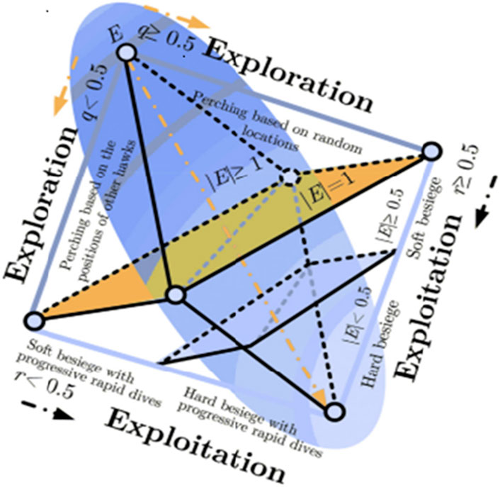
Figure 1. Principle of the HHO method (Heidari et al., 2019).
3.2.1 Exploration
Harris hawks watch over rabbits from their perches in tall branches. They choose two locate-and-capture strategies with equal chances of success. In the first strategy, the hawk creates a brand-new solution based on a random position, while in the second strategy, another hawk creates a solution based on its present optimal position and the mean of each agent. The following mathematical modeling can be considered to mimic such a scenario depicted in Equation 14.
where
where E is the escape energy, t is the number of iterations currently being performed, and
3.2.2 Exploitation
Hawks may restrict their prey during this stage, but the animals constantly try to elude the hawks using various methods. Therefore, the optimizer identifies four potential strategies to counteract these methods. Let r be the likelihood that a prey will escape an unexpected attack; in this case, if the likelihood is equal to or greater than 0.5, it signifies that the prey can successfully evade attack; conversely, this attempt is deemed unsuccessful if the probability is less than 0.5. However, unless a prey is specifically targeted, hawks always circle their prey. The E value for this situation is used to decide whether to besiege the prey softly or firmly. Thus,
3.2.2.1 Soft besiege
When both r and
3.2.2.2 Hard besiege
In this stage, r
3.2.2.3 Soft besiege with progressive rapid dives
During this stage, r
where S is a vector of size 1
In the above expression,
3.2.2.4 Hard besiege with progressive rapid dives
Under this condition,
Then, Y′ and Z′ are obtained using Equations 23, 24, respectively.
3.3 Motivation for the improved HHO algorithm based on OBL and iHHO
Most of the metaheuristic algorithms start with a random variable for initialization and corresponding distribution. Recently, chaotic mapping has been used in such metaheuristic techniques as it allows similar properties and characteristics as randomness, with improved dynamic and statistical performances. Therefore, chaotic mapping is added to the unique swarm intelligence approach in place of a random variable. As added advantages to the optimization strategy, this mapping offers accurate initialization, arbitrariness, and ergodicity (Baliarsingh and Vipsita, 2020). By producing non-repeated numbers with periodicity, chaotic mapping enhances the efficiency with respect to a random number. These characteristics resulting from chaotic mapping provide the means to escape local optima and preserve distinction while increasing the efficacy of the global search. Appropriate initialization is achieved when the preliminary points are adjusted such that a meaningful result is generated, assuming that the outcome is wisely dependent on the preliminary points. Throughout the phase of arbitrariness, chaotic mapping takes on the roles of the random variables. Ergodicity describes the capacity of a chaotic variable to identify non-repeated values given a specific range.
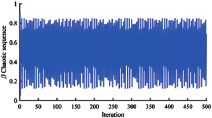
Different metaheuristic methods have been used to implement various chaotic functions. Recently, Zahmoul et al. (2017) reported a new approach to the family of chaotic functions; Equation 25 provides the mathematical representation of this mapping:
where
where c is the bifurcation parameter;
Exploration and exploitation are appropriately balanced when chaotic mapping is applied to the traditional HHO algorithm. Chaotic mapping replaces the random functions employed in traditional HHO techniques. Then, the constants q,
A fresh and practical theory for improving the performances of diverse metaheuristic approaches from an optimization standpoint is OBL. The idea of OBL is to take the opposite candidate as an alternative approach to reach the optimal solution, which could be closer to the global optimum solution. The objective of OBL in optimization is to improve the solution’s effectiveness by evaluating the contender for the solution of the relevant pair. The ideal response candidate is taken into account for the subsequent individual solution (Barisal and Prusty, 2015). Suppose that
The global searchability is enhanced with OBL, and the solution using this method with chaotic mapping is shown in Equation 31. In this instance,
4 Frequency estimation modeling
The instantaneous voltage signals of the three phases of a power system can be expressed as follows:
where the peak values of the three-phase voltage signals at the time instant n are denoted by the variables
Applying Clarke’s transform to the three-phase voltage signals in Equation 32 results in the complex-valued power system voltage signal (also known as the
In the complex-valued voltage signal,
In the above expression,
The input vector is updated by following the imLMS weight updating equation as stated in Equations 11, 12. Therefore the observed voltage signal and error [e(k) = d(k)-y(k)] is also updated in each Kth iteration. In the process, iHHO optimizer is also introduced in the weight updating equation. Thus, the process becomes effective and efficient. When the mean square error approximates to zero, the optimizer provides the optimal step sizes which automatically fetch to the weight updating equation and the system power frequency will be estimated using Equation 36.
The general steps involved in the proposed estimator are as follows:
Step (1). Initialization of the input vector, weight vector, and all variables.
Step (2). Formulation of the instantaneous voltage signal using Equation 32.
Step (3). Decomposition of voltage signal into its complex form using Equation 33.
Step (4). Conceptualization of the observed voltage signal through Equation 35.
Step (5). Updating the weight vector using the imFLMS estimator as per Equation 11.
Step (6). Optimal tuning of the step size and fractional-order step size with the optimization algorithm.
Step (7). Calculation of the frequency component from the weight update equation using Equation 36.
5 Summary of results and discussion
5.1 Validation of the proposed improved HHO algorithm
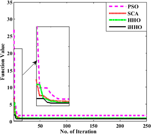
The improved HHO algorithm was used to obtain the optimal step size that minimizes the cost function of the proposed imFLMS estimation algorithm. Several distinct benchmark functions were used to verify the reliability and effectiveness of the proposed technique. The improved HHO showed greater optimal performance after 100 trials. The enhanced version is more accurate and resilient while requiring less processing time; the ideal solution demonstrates higher search process efficiency and flawless balance between exploration and exploitation while handling the benchmark functions. Figure 3 shows the convergence graph for comparison, where the optimization approach offers a more optimal value than the traditional HHO, SCA, and PSO techniques. The graphs show that the suggested iHHO algorithm maintains its ideal outcome in terms of fewer iterations and shorter execution time. The proposed optimizer was also applied to several common restricted benchmark functions, such as Mishra’s bird, Simionescu, and Townsend functions, as well as unconstrained benchmark functions like the Ackley, Levi, and Rastrigin functions (Pati and Subudhi, 2023). Their results show that the iHHO algorithm outperforms the other algorithms in terms of the best, worst, and mean values as well as execution time.
5.2 Temporal complexity of the proposed optimization algorithm
The temporal complexity of the proposed algorithm can be computed as follows and stated in Equation 37.
Thus, the algorithm performs
where O() represents the order;
5.3 Frequency estimation from three-phase balanced signals
Using filtering methods based on the LMS, mFLMS, and the newly proposed imFLMS algorithms, several examples of balanced power signals were simulated as follows.
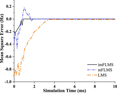
The control parameters of the weight update expression (
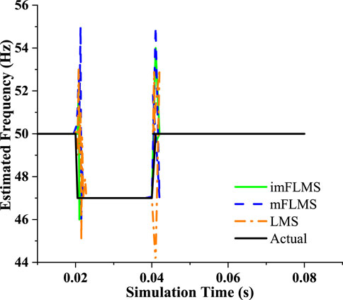
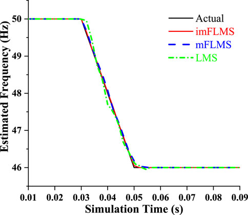
The power system signal with a fundamental frequency of 50 Hz was then applied with a step shift in frequency between 0.02 and 0.04 s, for which it was observed that the imFLMS estimation technique followed the frequency variation more closely than the other algorithms (Figure 7). Next, a ramp shift in frequency from 50 Hz to 46 Hz was applied between 0.03 and 0.05 s, following which the frequency was maintained constant at 46 Hz for the remainder of the period of the three-phase signal. As seen in Figure 8, the suggested technique successfully tracks the signal ramp change with a convergence time of less than half a cycle and a high degree of estimation accuracy. With the FLMS algorithm, the tracking began at about 0.033 s and leading to an inconsistent result. Similarly, as seen in the figure, the LMS algorithm followed the ramp variation from 0.038 s.
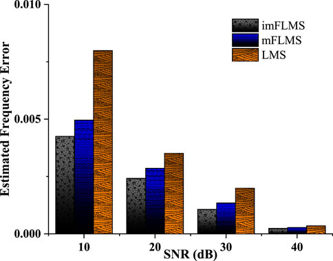
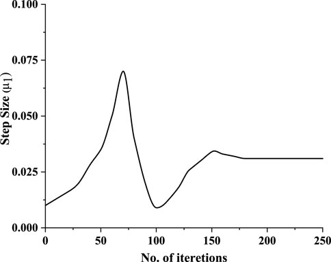
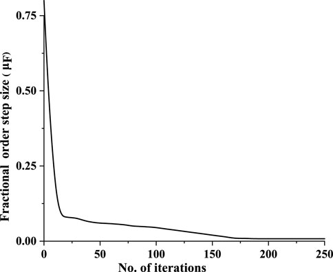
The step size variation
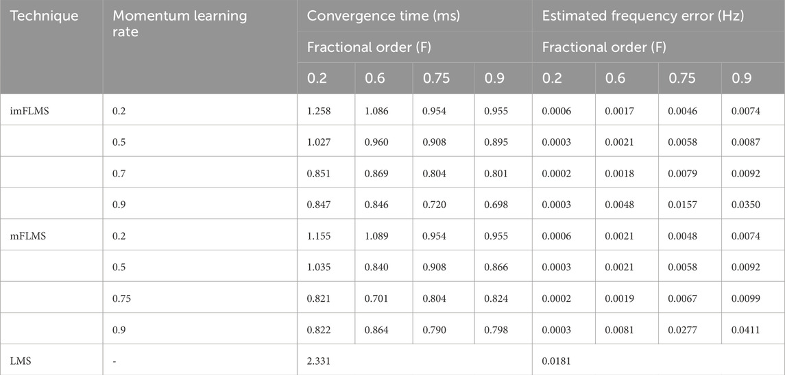
Table 2 displays the performance evaluation results for the suggested scheme in terms of the initial convergence rates for different momentum learning rates
5.4 Frequency estimation with a renewable-based power system
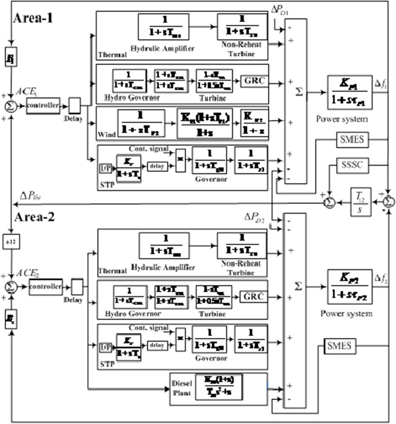
To examine the effectiveness of the proposed scheme, it was tested with a signal derived from a renewable-based two-area-load frequency control model. This power system was earlier modeled and simulated in MATLAB as well as evaluated by Pati and Subudhi (2021). Figure 11 shows the block diagram model of the test system under consideration (Pati and Subudhi, 2021).
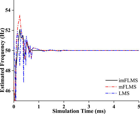
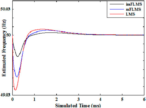
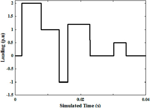
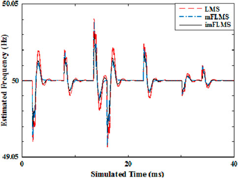
To validate the proposed scheme, a signal generated with a step load perturbation of 2% was considered and compared for the suggested imFLMS and existing estimation techniques. Figure 12 displays the relevant comparative plots for these estimation methods. Furthermore, the dynamic load signal shown in Figure 13 was applied to the test system to verify the algorithmic efficacy. The imFLMS, mFLMS, and LMS algorithms were used to estimate the test system frequency, and their results are shown in Figure 14. As verified earlier, the imFLMS algorithm outperforms the other estimation techniques; it estimates the frequency more precisely in less time than the other methods even with the random load, thus proving its robustness.
5.5 Experimental studies and results
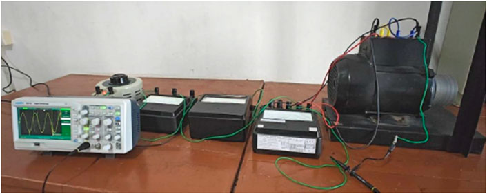
To validate the performance of the proposed algorithm for power system frequency estimation, a simple experimental setup was established in the laboratory. In this setup, an induction motor was connected as a load to a single-phase power supply, as suggested by Daw (2016). A variable AC supply was then employed to regulate the input voltage. A voltmeter, an ammeter, and a wattmeter were used to measure the output voltage, current, and power, respectively. The voltage signals were captured using a digital storage oscilloscope from the load side, where the induction motor was connected, as illustrated in Figure 15. The detailed specifications of the equipment used are as follows:
The input voltage waveform across the induction motor was recorded with a digital storage oscilloscope, and the data were subsequently transferred to a computer through communication software. Figure 16 illustrates the voltage signal estimation using the proposed imFLMS algorithm and the data obtained from the experiment. The results demonstrate that the proposed algorithm yields an estimation significantly closer to the actual signal and with a nearly identical period. Consequently, the fundamental frequency of 50 Hz was accurately estimated with minimal mean-squared error of 0.0741 Hz, indicating that the proposed estimator was highly effective for applications involving real-world data.
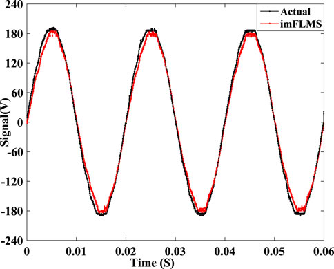
Figure 16. Actual waveform and estimated signal using the proposed method with the experimental setup.
5.6 Comparative assessment with state-of-the-art methods
The percentage improvement was measured in the comparative state-of-the-art study using Equations 38, 39, where
The results for the suggested adaptive scheme tuned by iHHO for power system frequency estimation were compared with those reported by Subudhi et al. (2020) and Nefabas et al. (2020). These comparisons are summarized in Table 4. Additionally, it has been demonstrated beyond reasonable doubt that the proposed method greatly enhances the reaction time of the system. Thus, we conclude that the suggested system configuration has better stability compared to those discussed in Subudhi et al. (2020) and Nefabas et al. (2020). From
6 Conclusion
This study presents a novel innovative momentum-learning-control-rate-based fractional-order LMS algorithm for instantaneous frequency estimation that was optimized using improved chaotic-based HHO. The proposed technique is suitable for measuring a wide range of frequency variations and exhibits superior behavior under dynamic conditions. The proposed algorithm was also investigated for step and ramp changes of the frequency signal with different noise levels. Thus, it was found to be a valuable and efficient tool for successful power frequency estimation, with the simulation results confirming the superior dynamic responses of the algorithm. The proposed estimation method with the chaotic and OBL with HHO shows better performance than the approach based on the simple LMS method for waveforms with noise. In addition, this approach is important for real-time signals from test systems. The investigations also verified the efficacy and improved performance of the suggested approach through comparisons with signals derived from a multiarea renewable-based power system model and real time experimental setup. The proposed algorithm is thus expected to be useful for system identification, noise cancellation, and real-time applications.
Data availability statement
The original contributions presented in the study are included in the article/Supplementary Material, and any further inquiries may be directed to the corresponding author.
Author contributions
SP: conceptualization, data curation, formal analysis, funding acquisition, investigation, methodology, project administration, resources, software, validation, visualization, writing–original draft, and writing–review and editing. US: conceptualization, formal analysis, funding acquisition, investigation, methodology, supervision, validation, writing–original draft, and writing–review and editing.
Funding
The authors declare that no financial support was received for the research, authorship, and/or publication of this article.
Conflict of interest
The authors declare that the research was conducted in the absence of any commercial or financial relationships that could be construed as a potential conflict of interest.
Publisher’s note
All claims expressed in this article are solely those of the authors and do not necessarily represent those of their affiliated organizations or those of the publisher, editors, and reviewers. Any product that may be evaluated in this article or claim that may be made by its manufacturer is not guaranteed or endorsed by the publisher.
References
Alabool, H. M., Alarabiat, D., Abualigah, L., and Heidari, A. A. (2021). Harris hawks optimization: a comprehensive review of recent variants and applications. Neural Comput. Appl. 33, 8939–8980. doi:10.1007/s00521-021-05720-5
Alhelou, H. H., Hamedani-Golshan, M. E., Njenda, T. C., and Siano, P. (2019). A survey on power system blackout and cascading events: research motivations and challenges. Energies 12, 682. doi:10.3390/en12040682
Alhussan, A. A., Farhan, A. K., Abdelhamid, A. A., El-Kenawy, E.-S. M., Ibrahim, A., and Khafaga, D. S. (2023). Optimized ensemble model for wind power forecasting using hybrid whale and dipper-throated optimization algorithms. Front. Energy Res. 11, 1174910. doi:10.3389/fenrg.2023.1174910
Aslam, M. S., Chaudhary, N. I., and Raja, M. A. Z. (2017). A sliding-window approximation-based fractional adaptive strategy for hammerstein nonlinear armax systems. Nonlinear Dyn. 87, 519–533. doi:10.1007/s11071-016-3058-9
Avalos, O., Cuevas, E., Becerra, H. G., Gálvez, J., Hinojosa, S., and Zaldívar, D. (2021). Kernel recursive least square approach for power system harmonic estimation. Electr. Power Components Syst. 48, 1–16. doi:10.1080/15325008.2021.1908457
Baliarsingh, S. K., and Vipsita, S. (2020). Chaotic emperor penguin optimised extreme learning machine for microarray cancer classification. IET Syst. Biol. 14, 85–95. doi:10.1049/iet-syb.2019.0028
Barisal, A. K., and Prusty, R. (2015). Large scale economic dispatch of power systems using oppositional invasive weed optimization. Appl. Soft Comput. 29, 122–137. doi:10.1016/j.asoc.2014.12.014
Bershad, N. J., Wen, F., and So, H. C. (2017). Comments on “fractional lms algorithm”. Signal Process. 133, 219–226. doi:10.1016/j.sigpro.2016.11.009
Chao, X., Xinze, X., Xin, H., and Can, D. (2024). Parameter identification method of load modeling based on improved dung beetle optimizer algorithm. Front. Energy Res. 12, 1415796. doi:10.3389/fenrg.2024.1415796
Chaudhary, N. I., Raja, M. A. Z., He, Y., Khan, Z. A., and Machado, J. T. (2021). Design of multi innovation fractional lms algorithm for parameter estimation of input nonlinear control autoregressive systems. Appl. Math. Model. 93, 412–425. doi:10.1016/j.apm.2020.12.035
Chaudhary, N. I., Raja, M. A. Z., and Rehman Khan, A. U. (2015). Design of modified fractional adaptive strategies for hammerstein nonlinear control autoregressive systems. Nonlinear Dyn. 82, 1811–1830. doi:10.1007/s11071-015-2279-7
Cheng, S., Wei, Y., Chen, Y., Li, Y., and Wang, Y. (2017). An innovative fractional order lms based on variable initial value and gradient order. Signal Process. 133, 260–269. doi:10.1016/j.sigpro.2016.11.026
Daw, N. A. (2016). “Comparison of lab work and simulation results for speed control of single phase induction motor capacitor starting,” in 2016 17th international conference on sciences and techniques of automatic control and computer engineering (STA) (IEEE), 397–402.
Friedman, V. (1994). A zero crossing algorithm for the estimation of the frequency of a single sinusoid in white noise. IEEE Trans. Signal Process. 42, 1565–1569. doi:10.1109/78.286978
Han, Y., Luo, M., Zhao, X., Guerrero, J. M., and Xu, L. (2015). Comparative performance evaluation of orthogonal-signal-generators-based single-phase pll algorithms—a survey. IEEE Trans. Power Electron. 31, 3932–3944. doi:10.1109/tpel.2015.2466631
Heidari, A. A., Mirjalili, S., Faris, H., Aljarah, I., Mafarja, M., and Chen, H. (2019). Harris hawks optimization: algorithm and applications. Future gener. Comput. Syst. 97, 849–872. doi:10.1016/j.future.2019.02.028
Kanoongo, S., and Giri, R. K. (2023). Link quality improvement analysis of relay-assisted hybrid rf/fso systems in challenging environments. Optik 294, 171442. doi:10.1016/j.ijleo.2023.171442
Li, J., Teng, Z., Wang, Y., You, S., Liu, Y., and Yao, W. (2019). A fast power grid frequency estimation approach using frequency-shift filtering. IEEE Trans. Power Syst. 34, 2461–2464. doi:10.1109/tpwrs.2019.2892599
Man, J., Chen, L., Terzija, V., and Xie, X. (2021). Mitigating high-frequency resonance in mmc-hvdc systems using adaptive notch filters. IEEE Trans. Power Syst. 37, 2086–2096. doi:10.1109/tpwrs.2021.3116277
Martinek, R., Rzidky, J., Jaros, R., Bilik, P., and Ladrova, M. (2019). Least mean squares and recursive least squares algorithms for total harmonic distortion reduction using shunt active power filter control. Energies 12, 1545. doi:10.3390/en12081545
Menesy, A. S., Sultan, H. M., Selim, A., Ashmawy, M. G., and Kamel, S. (2019). Developing and applying chaotic harris hawks optimization technique for extracting parameters of several proton exchange membrane fuel cell stacks. IEEE Access 8, 1146–1159. doi:10.1109/ACCESS.2019.2961811
Mojiri, M., Karimi-Ghartemani, M., and Bakhshai, A. (2007). Estimation of power system frequency using an adaptive notch filter. IEEE Trans. Instrum. Meas. 56, 2470–2477. doi:10.1109/tim.2007.908631
Naik, P. A., Zehra, A., Farman, M., Shehzad, A., Shahzeen, S., and Huang, Z. (2024). Forecasting and dynamical modeling of reversible enzymatic reactions with a hybrid proportional fractional derivative. Front. Phys. 11, 1307307. doi:10.3389/fphy.2023.1307307
Nefabas, G. L., Zhao, H., and Xia, Y. (2020). Widely linear least mean kurtosis-based frequency estimation of three-phase power system. IET Generation, Transm. and Distribution 14, 1159–1167. doi:10.1049/iet-gtd.2018.6498
Pan, X., Zhang, L., and Huang, H. (2021). Harmonic cancellation by adaptive notch filter based on discrete wavelet packet transform for an mmcc-statcom. IEEE Trans. Power Deliv. 37, 1834–1844. doi:10.1109/tpwrd.2021.3099201
Pati, S. S., and Subudhi, U. (2021). “Frequency regulation of solar-wind integrated multi-area system with smes and sssc,” in 2021 IEEE international power and renewable energy conference (IPRECON) (IEEE), 1–4.
Pati, S. S., and Subudhi, U. (2023). Stability analysis of a multi-area renewable system and frequency control with improved chaotic harris hawk optimization algorithm. Arabian J. Sci. Eng. 49, 6531–6550. doi:10.1007/s13369-023-08313-7
Sharma, R., Sethares, W. A., and Bucklew, J. A. (1998). Analysis of momentum adaptive filtering algorithms. IEEE Trans. Signal Process. 46, 1430–1434. doi:10.1109/78.668805
Shehab, M., Mashal, I., Momani, Z., Shambour, M. K. Y., AL-Badareen, A., Al-Dabet, S., et al. (2022). Harris hawks optimization algorithm: variants and applications. Archives Comput. Methods Eng. 29, 5579–5603. doi:10.1007/s11831-022-09780-1
Subudhi, U., Sahoo, H. K., and Mishra, S. K. (2020). Adaptive three-phase estimation of sequence components and frequency using h∞ filter based on sparse model. J. Mod. power Syst. clean energy 8, 981–990. doi:10.35833/mpce.2018.000440
Tan, Y., He, Z., and Tian, B. (2015). A novel generalization of modified lms algorithm to fractional order. IEEE Signal Process. Lett. 22, 1244–1248. doi:10.1109/lsp.2015.2394301
Wold, J., and Wilches-Bernal, F. (2021). Enhanced nonlinear least squares for power system frequency estimation with phase jump immunity. Int. J. Electr. Power and Energy Syst. 129, 106876. doi:10.1016/j.ijepes.2021.106876
Xie, J., Wei, X., Bo, X., Zhang, P., Chen, P., Hao, W., et al. (2023). State of charge estimation of lithium-ion battery based on extended kalman filter algorithm. Front. Energy Res. 11, 1180881. doi:10.3389/fenrg.2023.1180881
Xu, L., and Song, G. (2020). A recursive parameter estimation algorithm for modeling signals with multi-frequencies. Circuits, Syst. Signal Process. 39, 4198–4224. doi:10.1007/s00034-020-01356-3
Zahmoul, R., Ejbali, R., and Zaied, M. (2017). Image encryption based on new beta chaotic maps. Opt. Lasers Eng. 96, 39–49. doi:10.1016/j.optlaseng.2017.04.009
Zhang, S., Zhang, J., Zheng, W. X., and So, H. C. (2019). Widely linear complex-valued estimated-input lms algorithm for bias-compensated adaptive filtering with noisy measurements. IEEE Trans. Signal Process. 67, 3592–3605. doi:10.1109/tsp.2019.2919412
Zhang, X., Ding, Q., Luo, H., Hui, B., Chang, Z., and Zhang, J. (2017). Infrared small target detection based on directional zero-crossing measure. Infrared Phys. and Technol. 87, 113–123. doi:10.1016/j.infrared.2017.09.016
Zhao, J., Gómez-Expósito, A., Netto, M., Mili, L., Abur, A., Terzija, V., et al. (2019). Power system dynamic state estimation: motivations, definitions, methodologies, and future work. IEEE Trans. Power Syst. 34, 3188–3198. doi:10.1109/tpwrs.2019.2894769
Keywords: frequency estimation, improved momentum learning rate, fractional least mean squares algorithm, Harris hawks optimization, chaotic map, opposition-based leaning
Citation: Pati SS and Subudhi U (2024) Robust-momentum-learning-rate-based adaptive fractional-order least mean squares approach for power system frequency estimation using chaotic Harris hawks optimization. Front. Energy Res. 12:1467637. doi: 10.3389/fenrg.2024.1467637
Received: 20 July 2024; Accepted: 30 August 2024;
Published: 26 September 2024.
Edited by:
Soumya Ranjan Das, Parala Maharaja Engineering College (P.M.E.C), IndiaReviewed by:
Hemanta Kumar Sahu, VIT University, IndiaBijayananda Patnaik, National Institute of Technology Raipur, India
Copyright © 2024 Pati and Subudhi. This is an open-access article distributed under the terms of the Creative Commons Attribution License (CC BY). The use, distribution or reproduction in other forums is permitted, provided the original author(s) and the copyright owner(s) are credited and that the original publication in this journal is cited, in accordance with accepted academic practice. No use, distribution or reproduction is permitted which does not comply with these terms.
*Correspondence: Umamani Subudhi, dW1hbWFuaUBpaWl0LWJoLmFjLmlu
 Subhranshu Sekhar Pati
 Umamani Subudhi
