- 1School of Mechanical Engineering, Shanghai Jiao Tong University, Shanghai, China
- 2School of Nuclear Science and Engineering, Shanghai Jiao Tong University, Shanghai, China
Introduction: In the domain of nuclear power plant operations, accurately and rapidly predicting future states is crucial for ensuring safety and efficiency. Data-driven methods are becoming increasingly important for nuclear power plant parameter forecasting. While Transformer neural networks have emerged as powerful tools due to their self-attention mechanisms and ability to capture long-range dependencies, their application in the nuclear energy field remains limited and their capabilities largely untested. Additionally, Transformer models are highly sensitive to data complexity, presenting challenges for model development and computational efficiency.
Methods: This study proposes a feature selection method that integrates clustering and mutual information techniques to reduce the dimensionality of training data before applying Transformer models. By identifying key physical quantities from large datasets, we refine the data used for training a Transformer model, which is then optimized using the Tree-structured Parzen Estimator algorithm.
Results: Applying this method to a dataset for predicting a shutdown condition of a nuclear power plant, we demonstrate the effectiveness of the proposed “feature selection + Transformer” approach: (1) The Transformer model achieved high accuracy in predicting nuclear power plant parameters, with key physical quantities such as temperature, pressure, and water level attaining a normalized root mean squared error below 0.009, indicating that the RMSE is below 0.9% of the range of the original data, reflecting a very small prediction error. (2) The feature selection method effectively reduced input data dimensionality with minimal impact on model accuracy.
Discussion: The results demonstrate that the proposed clustering and mutual information-based method provides an effective feature selection strategy that encapsulates operational information of the plant.
1 Introduction
Nuclear power plants (NPPs) play a crucial role in meeting global energy demands while contributing to low-carbon electricity generation. Accurate prediction of operational states is critical for enhancing safety and efficiency in NPPs. This approach aims to improve current operations, support future autonomous control systems, and enable real-time monitoring. By facilitating rapid forecasting, it contributes to NPP automation, advancing safety, efficiency, and sustainable energy production in the nuclear industry.
In the domain of nuclear energy, forecasting methodologies generally fall into two categories: model-driven and data-driven approaches. Model-based predictions, when simplified for faster computational speed, often come with the caveat of substantial errors due to the simplification of physical models. On the other hand, more detailed models demand extensive computational resources, impeding the ability to forecast swiftly (Song et al., 2023). With recent technological advancements, particularly in data analytics and machine learning, we now have unprecedented capabilities to forecast and optimize NPP operations with improved precision and reliability. Data-driven methods can better handle the complexities and uncertainties in NPP operations compared to traditional model-driven approaches, as well as complex interactions between various operating parameters (e.g., temperature, pressure, flow rate) that are often challenging to fully account for in purely physics-based models.
Recent years have seen a proliferation of model-free machine learning approaches, demonstrating promising results conducive to NPP applications. Notably, deep learning models such as long short-term memory (LSTM) (Lei et al., 2022; Nguyen et al., 2021) and gated recurrent unit (GRU) (Kaminski and Diab, 2024) are well-suited for handling sequential data and have demonstrated exceptional performance in time series prediction tasks, which is why they are widely applied in predicting parameters of NPPs. Several studies highlight the effectiveness of these approaches. For instance, Liu et al. (2015) develops a dynamic model with dual back-propagation neural networks for continuous prediction of NPP operating parameters, including coolant void fraction, water level in steam generators, and pressurizers. Moshkbar-Bakhshayesh (2019) evaluates various supervised learning methods for forecasting NPP operating parameters. Bae et al. (2021) develops a data-driven prediction model using LSTM networks for fast and accurate forecasting of future parameter trends in NPPs, enhancing operator decision-making and potentially reducing human error in emergency situations. Li et al. (2022a) presents an automated deep learning approach for short-term prediction of thermal hydraulic parameters, achieving a maximum prediction error of about 4% and an average prediction time of 0.7 ms. Song et al. (2023) illustrates the GRU network’s ability to predict the future state of steam generators in NPPs based on measured data; Kim and Kim (2023) presents an algorithm that predicts and quantifies the uncertainty of NPP parameters over 2 h with high accuracy, using a blend of bidirectional LSTM, attention mechanisms, and a conditional variational autoencoder. Although models like LSTM excel in sequence comprehension, they may falter when broad context is needed, particularly in capturing long-term dependencies. This limitation is addressed by the Transformer architecture (Vaswani et al., 2017) with its robust self-attention mechanism that accurately captures complex contexts.
The Transformer model, originally developed for natural language processing, has recently emerged as a promising tool in time series forecasting. Characterized by its self-attention mechanism, the Transformer excels at capturing long-range dependencies in data (Wu et al., 2021), making it particularly suited for complex temporal relationships in NPP operational data. This ability potentially overcomes the limitations of traditional recurrent neural network models, offering improvements in prediction accuracy across various fields (Li et al., 2022b; Zeng et al., 2023). Several studies have demonstrated the superiority of Transformer models over traditional methods in various forecasting tasks. Zhao et al. (2021) points out the accuracy of Transformer models in short-term load forecasting, underscoring its advantages over regression-based models and traditional methods. Shen and Wang (2022) highlights how Transformer models, when integrated with classic CNN architectures, significantly improve time series forecasting, showing their superiority over traditional approaches. Mazen et al. (2023) shows the advantages of integrating Transformer models with GRU units for solar power forecasting, showing the Transformer’s superior handling of complex patterns over traditional models. Lim and Zohren (2021) reviews deep learning approaches for time series forecasting, particularly noting the superior performance of Transformer models in capturing long-range dependencies compared to traditional ARIMA and exponential smoothing methods. Despite its success in various domains, the adoption of Transformer models within the nuclear energy sector remains relatively nascent. Some notable applications include: Yi et al. (2023) discusses the application of Transformer-based models for detecting anomalies in NPP operational data, showcasing the model’s effectiveness in handling complex datasets; Aizpurua et al. (2019) integrates machine learning techniques, including Transformer models, for predicting the lifespan of power transformers within nuclear facilities, addressing operational parameter prediction; Tohver et al. (2023) employ the Temporal Fusion Transformer to forecast critical parameters of NPPs with high accuracy, enabling clear distinction among various accident scenarios and offering significant insights for enhancing operations; Xing et al. (2023) created a network model based on the Transformer architecture, aimed at predicting essential safety parameters in pressurized water reactor (PWR), which effectively forecasts the trends in water levels within pressurizers. In this paper, we employ Transformer as a predictive model to assess its suitability for operational data in NPPs. Despite its advantages, Transformer faces high computational complexity when dealing with long sequences (Cao et al., 2024).
To address this issue, feature selection can be employed. This approach is particularly relevant for NPP data management, which is characterized by diverse data sources, strong variable interdependencies, and low data value density (He et al., 2021). By retaining only key physical quantities, feature selection reduces the dimensionality of data, naturally decreasing the model’s computational complexity and shortening prediction times. From a view of machine learning, by selecting a subset of relevant features from the original data, feature selection also retains physical interpretability while improving learning performance, preventing overfitting, reducing computational costs, and minimizing memory usage without substantial loss of information (Li et al., 2017). Advancements in feature selection techniques have further enhanced the predictive capabilities of machine learning models across various domains: Mohamad et al. (2023) presents a hybrid physics-informed method for fault diagnostics in rotor-bearing systems, integrating physics and data-based techniques for feature extraction, ranking, and selection to improve fault classification accuracy across various operating conditions; Zha et al. (2022) proposes a wind power forecasting method using feature selection with the eXtreme Gradient Boosting (XGBoost) algorithm, improving forecast accuracy and reducing computational time; Lin and Li (2021) presents a Hybrid Kmeans-GRA-SVR method for short-term photovoltaic power generation forecasting, integrating feature selection to improve forecast accuracy and reduce training time compared to standard SVR models under ideal and non-ideal weather conditions. In the context of NPPs, Ramezani et al. (2023) evaluates multiple feature selection techniques to enhance the identification of transients in NPPs using deep learning models. He et al. (2021) proposes a correlation-based feature selection algorithm for NPP operating data, improving computational efficiency and generalization ability in machine learning applications. In this study, we explore the combination of Transformer models and feature selection techniques to address the specific challenges in NPP forecasting. This integrated approach aims to leverage the Transformer’s ability to capture complex temporal patterns while using feature selection to manage large-scale datasets efficiently.
To enhance the model’s predictive accuracy and generalization capability, this study employs the Tree-structured Parzen Estimator (TPE) algorithm for hyperparameter optimization during the training process. TPE, a sophisticated Bayesian optimization technique (Nguyen et al., 2020), has garnered attention for its remarkable search efficiency and adaptability across diverse domains. Recent applications of TPE have demonstrated its versatility and power: in agricultural sciences, it has improved soil water content estimation when combined with CatBoost algorithms (Yu et al., 2022); in environmental studies, it has accurately predicted biochar’s impact on N2O mitigation in constructed wetlands (Jiang et al., 2024); and in soil science, it has enhanced XGBoost model performance for salinity estimation through optimized feature selection and hyperparameter tuning (Chen et al., 2022). In the energy sector, TPE has significantly contributed to ultra-short-term wind power forecasting when integrated with XGBoost and Temporal Convolutional Networks (Zha et al., 2022). Building on these successes, our research leverages TPE to optimize the Transformer model’s hyperparameters, aiming to maximize its performance in predicting NPP operational data.
In this study, we propose a Transformer-based prediction framework for nuclear power plant (NPP) operational forecasting. Our approach integrates a novel data preprocessing method (combining clustering and mutual information) to identify key operational data types. Using data from a shutdown case, we construct time series reflecting operational state changes. A Transformer-based neural network is then trained on this preprocessed data, with hyperparameters optimized using the Tree-structured Parzen Estimator (TPE) method. This framework aims to enhance NPP operational forecasting, contributing to improved safety, efficiency, and potential future autonomous control systems.
This paper is structured as follows: Section 2 introduces the components of the proposed method, including the framework, feature extraction methods, neural network model, and optimization algorithm. Section 3 presents an overview of the operational data from NPPs used in this study. Section 4 discusses the results obtained from this method. Finally, Section 5 presents the conclusions drawn from the study.
2 Methods
2.1 Framework
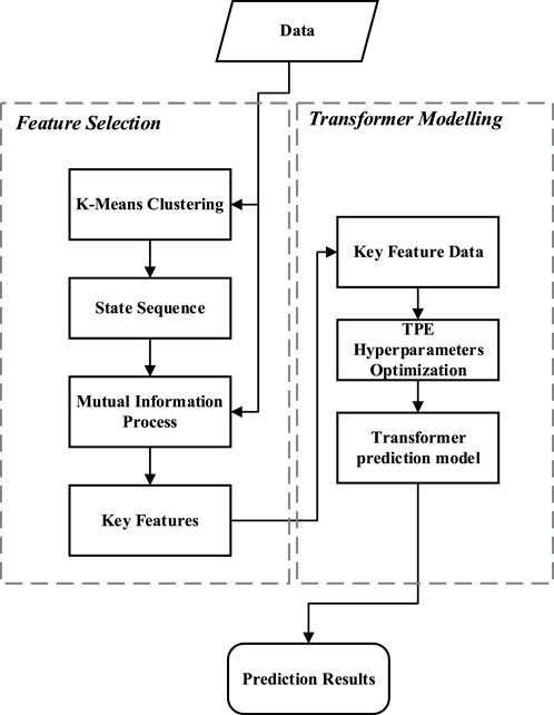
The proposed framework utilizes time series measurement data of multiple physical quantities from NPP to select key features. Subsequently, a predictive model is established using the data of these key features to perform predictions. The basic flowchart of the framework is shown in Figure 1 and includes the following four main steps.
2.1.1 Creation of a state sequence through clustering analysis
In our dataset, each time step is represented by a vector, where each element corresponds to a distinct physical quantity. For example, with 12 monitored physical quantities, each time step is represented by a 12-dimensional vector. As shown in Figure 2A, at any given time step, several measurement points in the nuclear power plant (NPP) generate data. These points monitor different physical quantities such as pressure, temperature, and flow rate. The measurement values from all points at the same time are combined into a single vector, where each vector represents the operational state of the reactor at that moment. As time progresses, each time step produces a new vector, resulting in a series of vectors that capture the evolving state of the system. The dimensionality of each vector corresponds to the number of monitored physical quantities (i.e., the number of measurement points), and the number of vectors is determined by the number of time steps collected. Ideally, we aim to collect as many time steps as possible to build a historical dataset that covers a wide range of operational states, which is critical for subsequent clustering analysis.
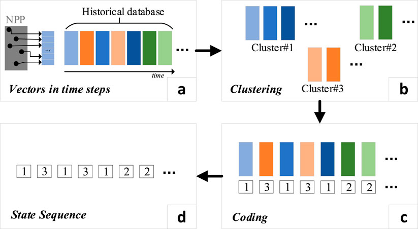
Figure 2. Generate state sequence from time series data. (A) Vectors in time steps. (B) Clustering. (C) Coding. (D) State sequence.
Before applying clustering, we normalize the data to ensure that all physical quantities are on comparable scales, as their units and magnitudes may differ significantly (e.g., pressure vs. flow rate). This step prevents any single variable from dominating the clustering process due to its larger numerical values. The details of the normalization procedure are described in Section 3 (“Datasets and Pre-processing”). After normalization, we apply the K-means clustering algorithm to group the 12-dimensional vectors (shown in Figure 2B). Each vector represents the system’s state at a specific time step, and the clustering groups these states based on their similarity (with Euclidean distance as the metric). The number of clusters (K) is determined using methods such as the silhouette score, which helps evaluate the cohesion and separation of clusters. In this study, we found that K = 3 provided the most meaningful grouping of operational states.
The result of the clustering process is a set of clusters, each representing a group of similar time steps. These clusters are then used to construct a state sequence, which provides a simplified representation of the NPP’s operational states (Figures 2C, D). Details of the clustering implementation are provided in Section 2.2.
The state sequence derived from clustering offers two main advantages over using the original time-series data for feature selection: it simplifies the process of correlating physical quantities with the reactor’s operational states, and it facilitates the calculation of mutual information for identifying key physical variables.
First, the selection of key physical quantities is based on their relevance to the reactor’s operational state. However, the operational state is not a single variable—it is the result of the complex interaction of multiple physical quantities. To represent this complexity, we use clustering to group the reactor’s operating conditions into distinct clusters, where each cluster represents a specific operational state. This allows us to transform the reactor’s continuous, high-dimensional operational data into a discrete state sequence, where each point in the sequence corresponds to a particular cluster. By using this state sequence, we can easily analyze the correlation between each individual physical quantity and the reactor’s operational states. Instead of trying to directly correlate a physical quantity’s time series with the entire multivariate dataset, we can now compare each physical quantity’s time series with the discrete state sequence, which simplifies the analysis process.
Second, we will use mutual information to quantify the relationship between each physical quantity and the reactor’s state transitions. Mutual information requires two sets of data—one representing the physical quantity and the other representing the reactor’s operational state. The state sequence serves this purpose perfectly, as it provides a discrete representation of the operational states. If we were to use the original time-series data directly, we would face the challenge of correlating a single variable’s time series with a high-dimensional dataset, which is both computationally complex and less intuitive. The state sequence reduces this complexity, making the mutual information calculation more efficient and meaningful.
2.1.2 Identification of key physical quantities using the state sequence
We use the state sequence, derived from clustering analysis, to identify critical physical quantities in the NPP operation. This process involves computing the mutual information between the state sequence and all individual time series data, shown in Figure 3. The physical quantities corresponding to the highest mutual information values are then selected as key features. This approach effectively pinpoints the most significant physical quantities that are strongly correlated with the NPP’s operational state, facilitating efficient feature selection for further analysis.

Figure 3. Calculate mutual information value of every physical quantities (features) with state sequence.
2.1.3 Modeling with key physical quantities
Using the selected critical physical quantities, we develop a Transformer-based neural network model for single-step time series prediction, forecasting the next time step based on a sequence of previous observations. The model is constructed and trained using data from the training and validation sets. To determine suitable hyperparameters, we employ the Tree-structured Parzen Estimator (TPE) algorithm. This optimization process covers Transformer architecture parameters (e.g., number of layers, number of heads in multi-head attention, hidden dimension), training parameters (e.g., learning rate, batch size). The TPE algorithm is used to search for a combination of these hyperparameters within predefined ranges, with the aim of minimizing the model’s validation loss.
2.1.4 Prediction on the test dataset
In the final phase, we apply the optimized model to the test set. The model generates predictions on this previously unseen data, and we calculate performance metrics to evaluate its predictive accuracy.
Overall, the process involves several steps of data collection, clustering, and feature selection to analyze the system’s operational states. The process begins with the collection of real-time measurements from n physical quantities over T time steps, forming the raw data matrix
2.2 K-means clustering
K-Means clustering (KMC) (Ahmed et al., 2020) is a popular and robust clustering algorithm that partitions data points into K clusters, optimizing for maximal intra-cluster similarity and minimal inter-cluster similarity. It iteratively adjusts cluster centroids to ensure each data point is assigned to the cluster with which it shares the most similarity. This unsupervised method is particularly effective for self-classification tasks. For instance, (Benmouiza and Cheknane, 2013), uses KMC to group the solar radiation time series in the research of solar radiation forecasting, dividing all data into three categories with meaningful solar radiation level or cloud condition; (Song et al., 2022); uses KMC to group NPP similar operational states in order to build specific prediction model on each subset.
The fundamental steps of KMC include selecting initial centroids, assigning data points to the nearest centroids, and updating the centroids until convergence. The formula (Equation 1) is:
where
The implementation process of KMC is as follows (Ahmed et al., 2020):
• Set the desired number of clusters K and select K data points as initial cluster centroids. Alternatively, randomly assign data points to K groups and compute the centroids for each group.
• Calculate the distances between all data points and the K centroids, assigning each point to the cluster with the closest centroid.
• Recalculate the centroids for each of the K clusters.
• Compare the new centroids with the previous centroids. If they remain the same, the process terminates; otherwise, return to second step.
In KMC, the predetermined number of clusters significantly influences the clustering outcome. In this study, the number of operational state types cannot be directly ascertained. Therefore, to more accurately represent working conditions, this paper adopts the silhouette coefficient to determine the optimal number of clusters.
The silhouette score (also silhouette coefficient) (Rousseeuw, 1987) is a metric for evaluating the quality of clustering results, commonly applied in algorithms like KMC. For example, silhouette scores are used in (Jin et al., 2022) for the clustering for categorization of source terms for risk assessment of NPPs. In (Choi and Seong, 2020), the silhouette score was used to determine the optimal number of clusters in hierarchical clustering analysis, contributing to the evaluation of operator fitness-for-duty in NPP scenarios. Silhouette score provides an objective measure of clustering efficacy by assessing both the cohesion within clusters and the separation between them. For each data point, the silhouette coefficient considers two crucial factors: the average distance to other points within the same cluster, reflecting intra-cluster similarity, and the average distance to points in the nearest cluster to which it does not belong, indicating inter-cluster dissimilarity. The formula (Equation 2) is:
where
The overall silhouette score is the mean of the silhouette scores of all individual samples in the dataset. If there are N samples, then the overall silhouette score S is given by:
2.3 Mutual information-based feature selection
During the operational process of an NPP, the collected data contains numerous features, not all of which are equally relevant to the NPP’s operational state. To enhance computational efficiency and focus on the most informative aspects, it is crucial to identify and select the features most closely associated with the NPP’s operational dynamics. This feature selection process builds upon the previously constructed state sequence, which reflects the NPP’s operational states over time. To accomplish this feature selection, we employ the mutual information method (Vergara and Estévez, 2014). This approach assesses the degree of association between each feature and the state sequence, identifying the features most relevant to the NPP’s operational states.
Mutual information is grounded in the concept of information entropy, quantifying the reduction in uncertainty about one random variable given knowledge of another. A high mutual information value indicates a strong relationship between two variables. The mutual information method is particularly effective at identifying relevant features while mitigating the effects of redundant information and noise. By comparing the joint probability distribution with the marginal probability distributions, it quantifies the contribution of each feature to the target variable through the calculated mutual information. Its formula (Equation 3) is:
where
The estimation of probability distributions is essential for the calculation of mutual information for time series data. Traditional methods like histogram-based approaches or kernel density estimation are often insufficient for capturing the complexities of time series data. Instead, more advanced techniques are typically employed. For continuous time series data, non-parametric methods such as the k-nearest neighbor (k-NN) approach (Ircio et al., 2020) or the Kraskov-Stögbauer-Grassberger (KSG) estimator (Kraskov et al., 2004) are frequently used. These methods avoid direct probability distribution estimation, making them suitable for high-dimensional data and complex dependencies often present in time series. In this study, probability estimation is performed using a k-nearest neighbors (k-NN) method to calculate the mutual information between each feature and the target variable (i.e., state sequence). This approach estimates the probability density function for each data point, capturing the dependencies between the data points without explicitly constructing probability distribution functions.
In brief, the k-NN method for density estimation is based on the idea that in high-density regions of data distribution, points are closer together, while in low-density regions, points are farther apart. This approach estimates density by observing the local distribution of data points. It assumes that points in high-density areas are closer to each other, while those in low-density areas are more distant. For each data point, the method finds its k nearest neighbors and calculates the volume of the smallest hypersphere containing these neighbors. The density estimate is inversely proportional to this volume. This technique is used to estimate the densities of the joint distribution
Important features are obtained for building a prediction model after feature selection by mutual information methods.
2.4 Transformer neural network
The Transformer architecture consists of two primary components: the encoder and the decoder. The encoder is composed of multiple identical layers, each containing a multi-head self-attention mechanism and a feed-forward network. The decoder follows a similar structure, with an additional multi-head encoder-decoder attention layer to facilitate interactions between input and output sequences. Figure 4 illustrates the key structural components and associated equations.
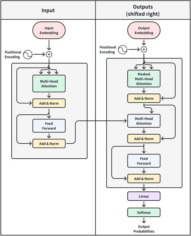
Figure 4. Transformer neural network (Vaswani et al., 2017).
The Transformer utilizes an attention mechanism, defined by Equation 4, where
Equations 5, 6 depict the multi-head attention mechanism within the Transformer architecture, where
The positional encoding in Transformer, added to the input embeddings, is defined by Equation 7:
Where
The feed-forward network (FFN) module in Transformer is represented by Equation 8:
where
The Transformer architecture, as described above, introduces several key hyperparameters that significantly influence its performance and efficiency. These include the number of encoder and decoder layers, the number of attention heads, the dimensionality of the model, the size of the feed-forward network. Additionally, training-specific hyperparameters such as learning rate, batch size, also play crucial roles. The optimal configuration of these hyperparameters can vary depending on the specific task and dataset. With the Transformer’s architecture defined, our focus now shifts to optimizing its performance through hyperparameter tuning. Techniques for neural network hyperparameter optimization will be discussed in Section 2.5.
2.5 Hyperparameter optimization by TPE
For hyperparameter optimization in neural networks, we employ the TPE method (Nguyen et al., 2020). TPE is a Bayesian optimization approach tailored for hyperparameter optimization. It constructs a probabilistic model with a tree-structured framework, iteratively refining the search space to pinpoint the best hyperparameter settings efficiently. The optimization procedure illustrated in Figure 5 involves the following steps:
(1) At the start-up iterations, a random search initializes the distribution by sampling the response surface
(2) Construct probability models
(3) For each hyperparameter set
(4) Iterate step 3, updating
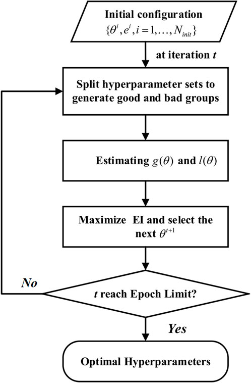
Figure 5. TPE parameter optimization flowchart (Nguyen et al., 2020).
Upon determining the optimal hyperparameters for the Transformer neural network, it will be utilized in the prediction model. The root mean squared error (RMSE) serves as the evaluation metric for assessing the Transformer model’s prediction outcomes.
3 Datasets and pre-processing
3.1 DataSets
In this study, the data we used comes from measurement data during the shutdown of an NPP: the main transformer trips, leading to the loss of the main off-site power, the onsite power automatically switches to the auxiliary power supply, the turbine trips, and the reactor is shut down.
The main event sequence is shown as Table 1. The insertion of control rods leads to the emergency shutdown of the reactor, with the nuclear power decreasing from 8.9%Pn to around 0%Pn. The main feedwater pumps of the secondary loop system stop, and the auxiliary feedwater system is activated. At this time, the coolant temperature drops, causing the pressure in the primary loop to decrease. After 678 s, when the pressurizer pressure drops below 14.6 MPa, the isolation valve acts, causing the pressurizer pressure to rise back to 15.5 MPa, after which the pressurizer pressure and water level again decrease with the drop in coolant temperature. Due to the decrease in feedwater flow rate to the steam generators on the secondary side, the heat absorption of the secondary loop decreases, causing the coolant temperature in the primary loop to rise. After 18,288 s, the heat transfer and heat dissipation in the primary loop gradually reach a dynamic balance, and the core thermal power also increases and stabilizes.
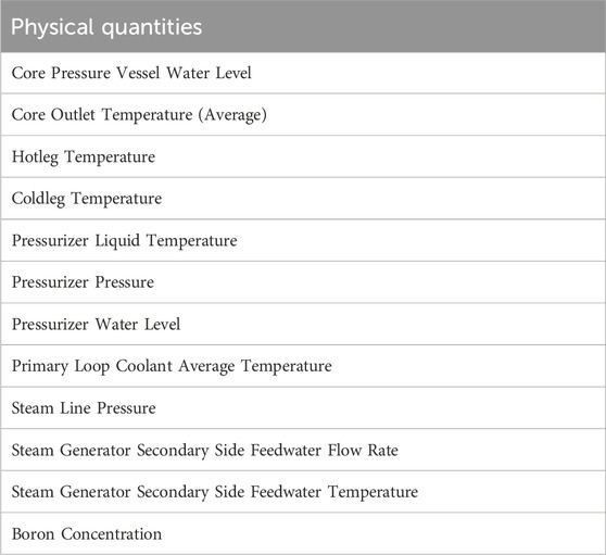
During the process, a total of 12 types of physical quantities, representing 12 features, were collected as listed in Table 2. Each type of data is in a time-series format, with a total of 2,000 time steps. The curves of these data are shown in Figures 6, 7.
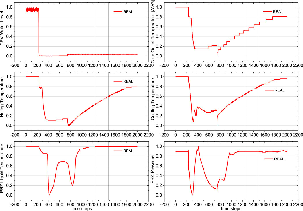
Figure 6. Curves for physical quantities 1–6, with vertical lines indicating the division into training (60%), validation (10%), and test (30%) sets.
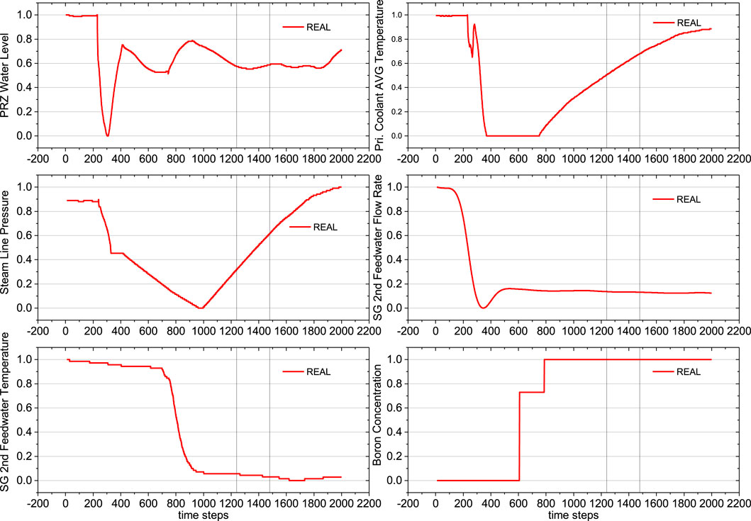
Figure 7. Curves for physical quantities 7–12, with vertical lines indicating the division into training (60%), validation (10%), and test (30%) sets.
To prevent information leakage and ensure unbiased model evaluation, we employ a three-way data split: training, validation, and test sets. The training and validation sets are used for model fitting and hyperparameter optimization, respectively. This approach keeps the test set independent, allowing for an accurate assessment of the model’s performance on unseen data. The dataset is divided into training, validation, and test sets in the ratio of 60%, 10%, and 30% respectively. The two vertical lines in the figures indicate this division.
3.2 Data pre-processing
To ensure that the measurements of different physical quantities are comparable and processed on the same scale, we apply Min-Max Normalization to each physical quantity. This method linearly transforms the data into a specified range, typically between 0 and 1. Specifically, for each physical quantity, the minimum value is mapped to 0, the maximum value is mapped to 1, and the other data points are scaled according to the following formula:
4 Results and discussion
In this Section, we use the aforementioned data to build and apply a prediction model. We first describe the process and results of feature selection in Section 4.1, followed by a description of the modeling process and prediction results of the Transformer model in Section 4.2.
4.1 Feature selection results
The first step involves clustering the 12-dimensional time series data. Based on the silhouette score analysis shown in Figure 8, the optimal number of clusters was found to be 3.
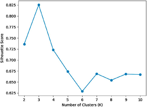
Figure 8. Silhouette score for different number of clusters. A higher Silhouette score indicates a better clustering.
Next, using KMC clustering, we cluster 2000 12-dimensional vectors into 3 groups, labeling them as Group 1, Group 2, and Group 3. Specifically, the visualization of clustering results for the time series is illustrated in Figure 9. Due to the difficulty in directly visualizing the clustering results of 12-dimensional vectors, in Figure 9A, we selected two normalized physical quantities (steam generator secondary side feedwater flow rate and temperature) to visualize the clustering results. With flow rate
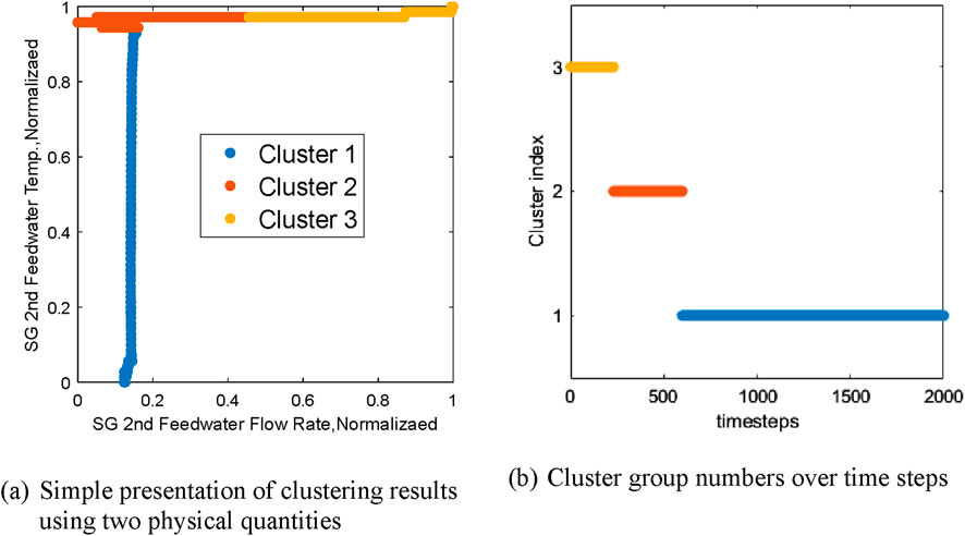
Figure 9. Visualization of clustering results used to generate the state sequence. (A) Simple presentation of clustering results using two physical quantities (B) Cluster group numbers over time steps.
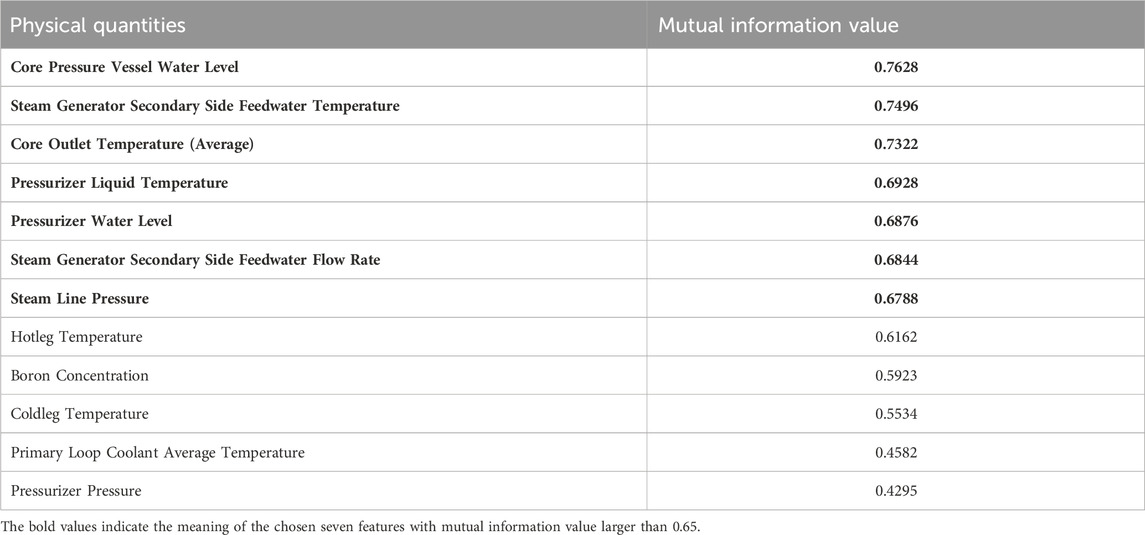
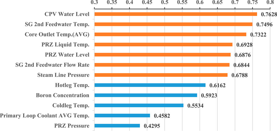
In the dataset of this study, the results were obtained through the calculation of mutual information in Table 3. Mutual information calculations were performed between the time series data of 12 physical quantities and the obtained state sequence, resulting in correlation values between the 12 physical quantities and the state. In this study, physical quantities with mutual information values above 0.65 were selected as important. The Core Pressure Vessel Water Level obtained the highest mutual information value of 0.7628, which may be due to its three distinct phases in the curve, which closely align with the division of time by the k-means clustering results, i.e., the state sequence.
Table 3 presents the mutual information calculations between the time series data of 12 physical quantities and the derived state sequence. These calculations quantify the correlation between each physical quantity and the state. Physical quantities with mutual information values exceeding 0.65 were deemed significant. This threshold was often chosen in correlation studies such as (Peng et al., 2018), which considers correlations above 0.6 as strong. We opted for 0.65 to ensure an even stronger correlation and to achieve better feature distinction, as illustrated in Figure 10. The Core Pressure Vessel Water Level exhibited the highest mutual information value of 0.7628. This strong correlation is likely attributable to its three distinct phases, which closely align with the temporal divisions produced by the k-means clustering in the state sequence.
Following the selection process via the mutual information method, this study has chosen seven types of data as primary for the next phase of prediction, highlighted in bold in Table 3. These include Core Pressure Vessel Water Level, Steam Generator Secondary Side Feedwater Temperature, Core Outlet Temperature (Average), Pressurizer Liquid Temperature, Pressurizer Water Level, Steam Generator Secondary Side Feedwater Flow Rate, and Steam Line Pressure.
4.2 Transformer modelling and prediction
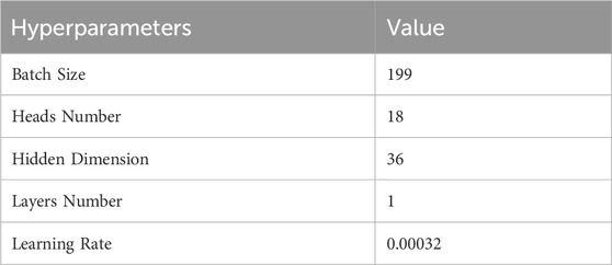
The prediction process employs a single-step forecasting approach. Once the optimal network is obtained through training and validation, it is employed to make single-step predictions on the test set. The performance evaluation involves comparing the predicted values with the actual values. Python is used as the programming language for implementation. The optimization process focuses on determining suitable hyperparameters, including batch size, number of heads, hidden dimension, number of layers, and learning rate. The relevant parameters for the TPE setup are as follows: TPE training generations number is 3,000, TPE iteration cycles number is 10 and model training generations number is 100,000. The optimal hyperparameters are finally found as shown in Table 4.
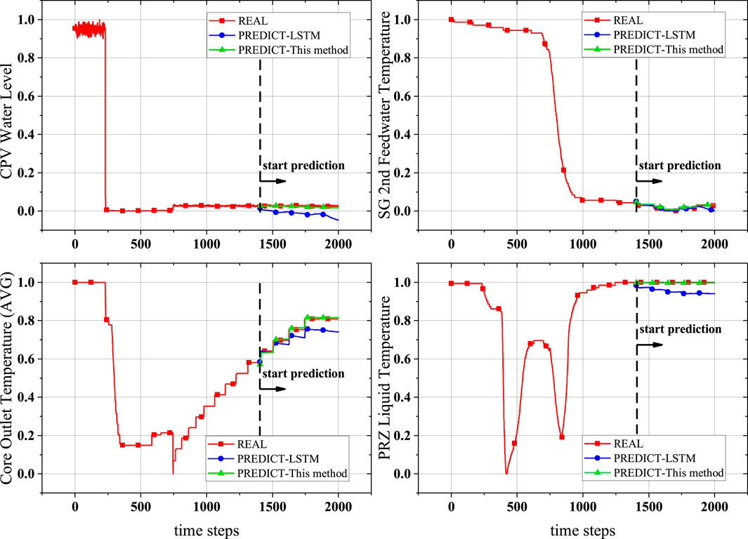
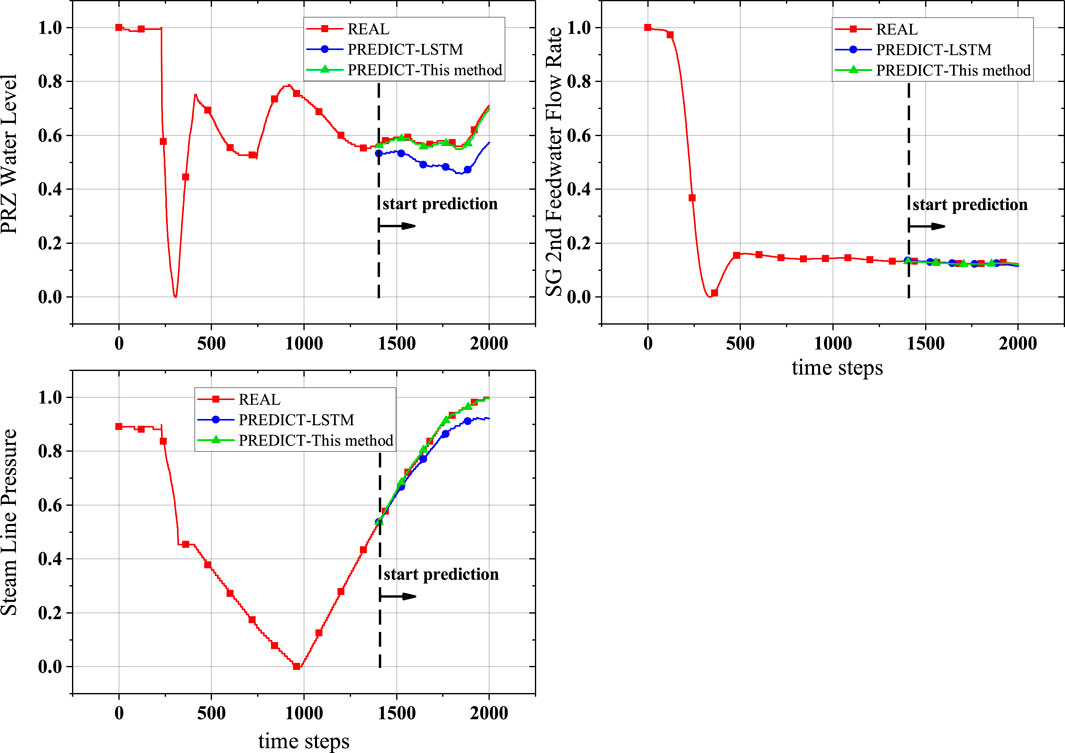
Next, the established neural network model was used for prediction. To evaluate its performance, we compared it with an LSTM model. The LSTM algorithm was selected as a benchmark due to its advanced capabilities in handling sequential data and its widespread use in time series forecasting. After undergoing a similar hyperparameter optimization process, an LSTM prediction model was obtained. This optimized LSTM model utilized a batch size of 187, 16 hidden units, 1 layers, and a learning rate of 0.00035. Its results on the test set were then compared with those of our method. The prediction results in the figures start from the test set (the 1400th time step), as the training and validation sets were used to build the model. The results of training the Transformer model (green lines) and the LSTM prediction results (blue lines) are shown in Figures 11, 12, highlighting significant differences from the actual data.
The comparison of RMSE between the LSTM and Transformer results is presented in Table 5. The data shows that our method’s Transformer prediction model has better predictive performance. It should be noted that the RMSE of normalized results represents the ratio of actual prediction error to the data range. This can be derived from the normalization equation
From Figures 11, 12, we can see that the prediction results of this method for almost every physical quantity align well with the actual data, where the red line represents the actual measured values (normalized) and the green line represents the predictions by the Transformer model. The good prediction results can be attributed to the powerful predictive capability of the Transformer model and possibly also to the single-step prediction mode. Whether the actual data is near-stable, rapidly increasing, or showing a stepwise rise, the Transformer model demonstrates excellent predictive performance. As seen in Table 5, the RMSE values of Transformer model are all below 0.0088, which could be seen as 0.88% of the data range, a very small error.
In the single-step prediction results, we observed significant differences between the Transformer and LSTM models. Although both models perform single-step predictions, their performance differences can be explained by the fundamental mechanisms of the models. LSTM relies on its internal state and the output from the previous time step at each time step. While single-step prediction can reduce cumulative errors, LSTM may still face challenges such as struggling to effectively utilize earlier historical information for long sequences and the gating mechanism not completely mitigating long-term dependency issues in some cases. This error accumulation is most evident in the core outlet temperature and steam pipe pressure. On the other hand, the Transformer utilizes a self-attention mechanism that allows it to fully leverage the entire historical sequence, even in single-step predictions. Its advantages include the ability to directly attend to any part of the input sequence, unrestricted by position; the capability to capture patterns at multiple time scales simultaneously through multi-head attention; and the ability to reassess the importance of the entire historical sequence for each prediction step. In this case, the Transformer demonstrated better prediction accuracy, likely because even in single-step predictions, the Transformer can more effectively leverage long-term historical information. The self-attention mechanism allows the model to dynamically adjust its focus on different historical time points for each prediction, reducing potential errors from sequential processing.
4.3 Further discussion
4.3.1 Clustering methods
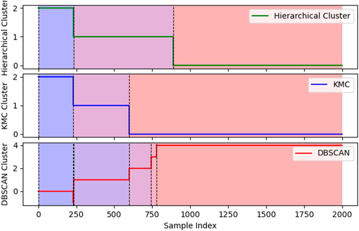
Here we elaborate on the choice of K-means clustering for state sequence generation. While K-means clustering was initially selected for its computational efficiency and ease of implementation, we conducted comparative experiments using other clustering methods, including hierarchical clustering and DBSCAN, to evaluate their relative performance.
4.3.1.1 Hierarchical clustering algorithm
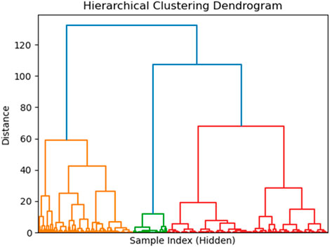
Hierarchical clustering is an agglomerative method that builds a hierarchy of clusters, where each data point starts as its own cluster and pairs of clusters are successively merged based on a linkage criterion. In this analysis, we used Ward’s method, which minimizes the total within-cluster variance, making it well-suited for generating compact clusters. The distance between clusters is represented by the increase in variance when clusters are merged. The dendrogram provides a visual representation (Figure 13) of the clustering process, with the height of the merges indicating the dissimilarity between clusters.
The dataset consists of 2,000 time steps, each described by 12 variables. Before clustering, the data was standardized using Z-score normalization to ensure that each feature contributes equally to the clustering process. The hierarchical clustering was performed using the Ward linkage method, and the dendrogram was constructed based on the resulting linkage matrix.
The dendrogram illustrates these clusters, with each branch representing the hierarchical merging process based on the distances between data points. The significant distance between certain branches suggests that the three clusters are distinct from each other. We chose to cut the dendrogram into three clusters based on the visual identification of a significant jump in the merge distances at a certain height. Note that the X-axis here does not represent time steps; instead, it shows sample indices, which do not necessarily follow any specific order and simply indicate the position of samples in the dataset. The clustering results show that the 2,000 time steps were grouped into three distinct clusters: 1 to 232, 233 to 888, 889 to 2,000.
4.3.1.2 DBSCAN
We also applied the DBSCAN (Density-Based Spatial Clustering of Applications with Noise) algorithm to cluster the dataset. DBSCAN is advantageous as it does not require predefining the number of clusters and can detect noise points (outliers) in the data. DBSCAN is well-suited for identifying clusters of arbitrary shapes and handling datasets with varying densities. The key parameters of DBSCAN are eps and min_samples. The eps defines the neighborhood radius around each point. If there are enough points within this radius (determined by min_samples), the point is considered a core point and forms part of a cluster. The min_samples specifies the minimum number of points required to form a dense region. Points that do not meet this requirement are classified as noise (labeled as −1).
In this experiment, after standardizing the data, DBSCAN identified several clusters, with some points labeled as noise. Clustering results: 1 to 229, 230 to 233 (noisy data), 234 to 598, 599 to 756, 757 to 2000. These noise points are likely isolated or outlier data points that do not belong to any cluster.
4.3.1.3 Comparison of different clustering methods
Figure 14 shows the comparison of three clustering methods. The same color in the chart represents the same cluster. By comparing the results of hierarchical clustering, K-means clustering (KMC), and DBSCAN, we can observe that K-means clustering provides sufficient performance in grouping the data. The first group on the far left is almost identical across all three methods, and all of them cluster the data after index 880 into a single large group. K-means and hierarchical clustering show very similar grouping patterns, both dividing the data into three main clusters. In comparison, the first two groups from the left in DBSCAN are almost perfectly aligned with the K-means results. While DBSCAN reveals more detailed groupings, each boundary point in K-means corresponds closely to a division point in DBSCAN. Furthermore, DBSCAN’s handling of noise (Cluster −1) did not significantly impact the overall structure in this dataset, indicating that K-means provides sufficiently clear clustering.
From a practical standpoint, K-means is an ideal choice for this dataset due to its simplicity and efficiency. It not only captures the main patterns in the data effectively but also avoids the computational complexity of hierarchical clustering and the parameter sensitivity of DBSCAN. Therefore, considering the high consistency of K-means with the other methods and its computational efficiency, K-means is more than adequate for meeting the clustering needs of this dataset.
4.3.2 Parameter selection and impact
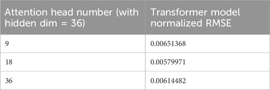
In this section, we discuss the effect of different parameter choices made for the Transformer model. Based on the optimal hyperparameters used in previous sections, we systematically varied two key parameters—training epochs and attention head numbers—to observe their impact on the model’s performance.
Effect of Training Epochs: The impact of training epochs on the performance of the Transformer model is evident in Table 6, where the normalized RMSE progressively decreases as the number of epochs increases. Specifically, after 100 epochs, the model achieves an RMSE of 0.0290. With further training, the RMSE drops significantly to 0.0123 at 500 epochs and continues to decrease to 0.0058 at 1,000 epochs. This consistent reduction in RMSE indicates that the model benefits from extended training, refining its ability to fit the data as the number of epochs increases. The results suggest that longer training enables the Transformer model to capture more intricate patterns in the data, leading to more accurate predictions. Notably, the substantial improvement between 500 and 1,000 epochs highlights the importance of sufficient training time for achieving optimal performance.
Effect of Attention Head Numbers: Table 7 demonstrates how the number of attention heads affects the model’s performance. Based on our previous hyperparameter search, 18 attention heads were identified as the optimal value. When using this number of heads, the model achieves the lowest normalized RMSE (0.0058). In contrast, using fewer attention heads (=9) results in a normalized RMSE of 0.0065, while increasing the number to 36 gives an RMSE of 0.0061. These results confirm that the number of attention heads is a critical hyperparameter in the Transformer model. Too few attention heads limit the model’s ability to capture diverse relationships in the input data, while too many heads introduce redundancy and potential overfitting. The best performance is achieved with 18 attention heads, indicating that this value strikes an ideal balance between model complexity and performance.
In summary, both training epochs and attention head numbers significantly affect the Transformer model’s performance. Increasing the training epochs consistently improves accuracy, while the number of attention heads has a more pronounced effect on the model’s ability to generalize and avoid overfitting. Given the importance of the attention mechanism in the Transformer model, an optimal number of attention heads is crucial for achieving the best prediction results.
5 Conclusion
This paper presents a combined feature selection and Transformer approach for predicting operational parameters of nuclear power plants. The K-means clustering method is employed to identify state sequences from the time series data of the power plant. Mutual information between each physical quantity and the state sequences is then calculated to select the key parameters strongly correlated with the plant’s operation. Based on these key parameters, a single-step prediction model is constructed using a Transformer neural network. The methodology is illustrated using data from a nuclear power plant shutdown caused by the loss of off-site power.
The results demonstrate that the proposed clustering and mutual information-based method provides an effective feature selection strategy that encapsulates operational information of the plant. From twelve physical quantities, seven critical ones highly correlated with the operational state were selected. The Transformer network, built on these selected parameters, achieved high prediction accuracy, with normalized RMSE values below 0.009 for critical physical quantities. This indicates that the RMSE is less than 0.9% of the original data range, reflecting a very small prediction error.
Although our study uses a relatively small number of parameters, it is important to note that the effectiveness of our feature selection method is not dependent on the number of features. The key advantage of our approach lies in its ability to incorporate operational state information of the nuclear power plant into the feature selection process. This method is also effective when dealing with large volumes of operational data that need to be reduced to a manageable size. Future work could explore the application of our method to datasets with a larger number of parameters to further demonstrate its scalability and effectiveness.
Despite the promising results presented in this study, there are several directions for improvement. (1) Feature Selection and Dimensionality Reduction: While the current approach successfully leverages clustering to reduce dimensionality, more advanced feature extraction techniques could be explored to handle increasingly complex and high-dimensional datasets. For instance, methods such as autoencoders or deep mutual information-based feature selection could complement the current approach by providing more robust and automated feature extraction, which may further improve the overall performance of the model on more intricate datasets. (2) Computational Efficiency: Although the clustering step alleviates some of the computational burden associated with training the Transformer model, further optimization is necessary when applying the model to larger datasets or real-time monitoring systems. Future research could explore more efficient Transformer variants, such as using sparse attention, model pruning, or lightweight attention mechanisms, to reduce computational costs while maintaining high prediction accuracy and scalability.
Data availability statement
The original contributions presented in the study are included in the article/supplementary material, further inquiries can be directed to the corresponding author.
Author contributions
YT: Conceptualization, Methodology, Software, Validation, Visualization, Writing–original draft. XL: Conceptualization, Data curation, Resources, Software, Supervision, Writing–original draft, Writing–review and editing.
Funding
The author(s) declare that no financial support was received for the research, authorship, and/or publication of this article.
Conflict of interest
The authors declare that the research was conducted in the absence of any commercial or financial relationships that could be construed as a potential conflict of interest.
The author(s) declared that they were an editorial board member of Frontiers, at the time of submission. This had no impact on the peer review process and the final decision.
Publisher’s note
All claims expressed in this article are solely those of the authors and do not necessarily represent those of their affiliated organizations, or those of the publisher, the editors and the reviewers. Any product that may be evaluated in this article, or claim that may be made by its manufacturer, is not guaranteed or endorsed by the publisher.
References
Ahmed, M., Seraj, R., and Islam, S. M. S. (2020). The k-means algorithm: a comprehensive survey and performance evaluation. Electronics 9, 1295. doi:10.3390/electronics9081295
Aizpurua, J. I., McArthur, S. D. J., Stewart, B. G., Lambert, B., Cross, J. G., and Catterson, V. M. (2019). Adaptive power transformer lifetime predictions through machine learning and uncertainty modeling in nuclear power plants. IEEE Trans. Industrial Electron. 66, 4726–4737. doi:10.1109/TIE.2018.2860532
Bae, J., Kim, G., and Lee, S. J. (2021). Real-time prediction of nuclear power plant parameter trends following operator actions. Expert Syst. Appl. 186, 115848. doi:10.1016/j.eswa.2021.115848
Benmouiza, K., and Cheknane, A. (2013). Forecasting hourly global solar radiation using hybrid k-means and nonlinear autoregressive neural network models. Energy Convers. Manag. 75, 561–569. doi:10.1016/j.enconman.2013.07.003
Cao, K., Zhang, T., and Huang, J. (2024). Advanced hybrid LSTM-transformer architecture for real-time multi-task prediction in engineering systems. Sci. Rep. 14, 4890. doi:10.1038/s41598-024-55483-x
Chen, B., Zheng, H., Luo, G., Chen, C., Bao, A., Liu, T., et al. (2022). Adaptive estimation of multi-regional soil salinization using extreme gradient boosting with Bayesian TPE optimization. Int. J. Remote Sens. 43, 778–811. doi:10.1080/01431161.2021.2009589
Choi, M. K., and Seong, P. H. (2020). A methodology for evaluating human operator’s fitness for duty in nuclear power plants. Nucl. Eng. Technol. 52, 984–994. doi:10.1016/j.net.2019.10.024
He, Y., Yu, H., Yu, R., Song, J., Lian, H., He, J., et al. (2021). A correlation-based feature selection algorithm for operating data of nuclear power plants. Sci. Technol. Nucl. Installations 2021, 1–15. doi:10.1155/2021/9994340
Ircio, J., Lojo, A., Mori, U., and Lozano, J. A. (2020). Mutual information based feature subset selection in multivariate time series classification. Pattern Recognit. 108, 107525. doi:10.1016/j.patcog.2020.107525
Jiang, B.-N., Zhang, Y.-Y., Zhang, Z.-Y., Yang, Y.-L., and Song, H.-L. (2024). Tree-structured parzen estimator optimized-automated machine learning assisted by meta–analysis for predicting biochar–driven N2O mitigation effect in constructed wetlands. J. Environ. Manag. 354, 120335. doi:10.1016/j.jenvman.2024.120335
Jin, K., Cho, J., and Kim, S. (2022). Machine learning-based categorization of source terms for risk assessment of nuclear power plants. Nucl. Eng. Technol. 54, 3336–3346. doi:10.1016/j.net.2022.04.006
Kaminski, M., and Diab, A. (2024). Time-series forecasting of a typical PWR undergoing large break LOCA. Sci. Technol. Nucl. Installations 2024, 1–16. doi:10.1155/2024/6162232
Kim, H., and Kim, J. (2023). Long-term prediction of safety parameters with uncertainty estimation in emergency situations at nuclear power plants. Nucl. Eng. Technol. 55, 1630–1643. doi:10.1016/j.net.2023.01.026
Kraskov, A., Stögbauer, H., and Grassberger, P. (2004). Estimating mutual information. Phys. Rev. E 69, 066138. doi:10.1103/PhysRevE.69.066138
Lei, J., Ren, C., Li, W., Fu, L., Li, Z., Ni, Z., et al. (2022). Prediction of crucial nuclear power plant parameters using long short-term memory neural networks. Intl J Energy Res. 46, 21467–21479. doi:10.1002/er.7873
Li, J., Cheng, K., Wang, S., Morstatter, F., Trevino, R. P., Tang, J., et al. (2017). Feature selection: a data perspective. ACM Comput. Surv. 50 (94), 1–45. doi:10.1145/3136625
Li, X., Cheng, K., Huang, T., Qiu, Z., and Tan, S. (2022a). Research on short term prediction method of thermal hydraulic transient operation parameters based on automated deep learning. Ann. Nucl. Energy 165, 108777. doi:10.1016/j.anucene.2021.108777
Li, X., Cheng, K., Huang, T., and Tan, S. (2022b). Research on false alarm detection algorithm of nuclear power system based on BERT-SAE-iForest combined algorithm. Ann. Nucl. Energy 170, 108985. doi:10.1016/j.anucene.2022.108985
Lim, B., and Zohren, S. (2021). Time series forecasting with deep learning: a survey. Phil. Trans. R. Soc. A 379, 20200209. doi:10.1098/rsta.2020.0209
Lin, J.-K., and Li, H. (2021). A hybrid K-Means-GRA-SVR model based on feature selection for day-ahead prediction of photovoltaic power generation. J. Comput. Commun. null 09, 91–111. doi:10.4236/jcc.2021.911007
Liu, T., Wei, H., Zhang, K., and Guo, W. (2016). “Mutual information based feature selection for multivariate time series forecasting,” in 2016 35th Chinese control conference (CCC), 7110–7114. doi:10.1109/ChiCC.2016.7554480
Liu, Y., Xie, F., Xie, C., Peng, M., Wu, G., and Xia, H. (2015). Prediction of time series of NPP operating parameters using dynamic model based on BP neural network. Ann. Nucl. Energy 85, 566–575. doi:10.1016/j.anucene.2015.06.009
Mazen, F. M. A., Shaker, Y., and Abul Seoud, R. A. (2023). Forecasting of solar power using GRU–temporal fusion transformer model and DILATE loss function. Energies 16, 8105. doi:10.3390/en16248105
Mohamad, T. H., Abbasi, A., Kappaganthu, K., and Nataraj, C. (2023). On extraction, ranking and selection of data-driven and physics-informed features for bearing fault diagnostics. Knowledge-Based Syst. 276, 110744. doi:10.1016/j.knosys.2023.110744
Moshkbar-Bakhshayesh, K. (2019). Comparative study of application of different supervised learning methods in forecasting future states of NPPs operating parameters. Ann. Nucl. Energy 132, 87–99. doi:10.1016/j.anucene.2019.04.031
Nguyen, H.-P., Baraldi, P., and Zio, E. (2021). Ensemble empirical mode decomposition and long short-term memory neural network for multi-step predictions of time series signals in nuclear power plants. Appl. Energy 283, 116346. doi:10.1016/j.apenergy.2020.116346
Nguyen, H.-P., Liu, J., and Zio, E. (2020). A long-term prediction approach based on long short-term memory neural networks with automatic parameter optimization by Tree-structured Parzen Estimator and applied to time-series data of NPP steam generators. Appl. Soft Comput. 89, 106116. doi:10.1016/j.asoc.2020.106116
Peng, B. S., Xia, H., Liu, Y. K., Yang, B., Guo, D., and Zhu, S. M. (2018). Research on intelligent fault diagnosis method for nuclear power plant based on correlation analysis and deep belief network. Prog. Nucl. Energy 108, 419–427. doi:10.1016/j.pnucene.2018.06.003
Ramezani, I., Vosoughi, N., Moshkbar-Bakhshayesh, K., and Ghofrani, M. B. (2023). Evaluation of the performance of different feature selection techniques for identification of NPPs transients using deep learning. Ann. Nucl. Energy 183, 109668. doi:10.1016/j.anucene.2022.109668
Rousseeuw, P. (1987). Silhouettes: a graphical aid to the interpretation and validation of cluster analysis. J. Comput. Appl. Math. 20, 53–65. doi:10.1016/0377-0427(87)90125-7
Shen, L., and Wang, Y. (2022). TCCT: tightly-coupled convolutional transformer on time series forecasting. Neurocomputing 480, 131–145. doi:10.1016/j.neucom.2022.01.039
Song, H., Liu, X., and Song, M. (2023). Comparative study of data-driven and model-driven approaches in prediction of nuclear power plants operating parameters. Appl. Energy 341, 121077. doi:10.1016/j.apenergy.2023.121077
Song, H., Song, M., and Liu, X. (2022). Online autonomous calibration of digital twins using machine learning with application to nuclear power plants. Appl. Energy 326, 119995. doi:10.1016/j.apenergy.2022.119995
Tohver, H., de Oliveira, R., and Jeltsov, M. (2023). Interpretable time series forecasting of NPP parameters in accident scenarios. Nucl. Eng. Des. 403, 112145. doi:10.1016/j.nucengdes.2022.112145
Vaswani, A., Shazeer, N., Parmar, N., Uszkoreit, J., Jones, L., Gomez, A. N., et al. (2017). “Attention is all you need,” in Advances in neural information processing systems. Editor I. Guyon, U. von Luxburg, S. Bengio, H. M. Wallach, R. Fergus, S. V. N. Vishwanathanet al. (Long Beach, CA: Curran Associates, Inc.). Available at: https://proceedings.neurips.cc/paper_files/paper/2017/hash/3f5ee243547dee91fbd053c1c4a845aa-Abstract.html.
Vergara, J. R., and Estévez, P. A. (2014). A review of feature selection methods based on mutual information. Neural Comput. and Applic 24, 175–186. doi:10.1007/s00521-013-1368-0
Wu, H., Xu, J., Wang, J., and Long, M. (2021). “Autoformer: decomposition transformers with auto-correlation for long-term series forecasting,” in Advances in neural information processing systems. Editor M. Ranzato, A. Beygelzimer, Y. N. Dauphin, P. Liang, and J. W. Vaughan (Curran Associates, Inc.), 22419–22430. Available at: https://proceedings.neurips.cc/paper/2021/hash/bcc0d400288793e8bdcd7c19a8ac0c2b-Abstract.html (Accessed April 15, 2024).
Xing, J., Li, W., Deng, S., Duan, P., and Ma, X. (2023). Research on forecasting approach of key parameters of PWR pressurizer water level. J. Phys. Conf. Ser. 2425, 012038. doi:10.1088/1742-6596/2425/1/012038
Yi, S., Zheng, S., Yang, S., Zhou, G., and He, J. (2023). Robust transformer-based anomaly detection for nuclear power data using maximum correntropy criterion. Nucl. Eng. Technol. 56, 1284–1295. doi:10.1016/j.net.2023.11.033
Yu, J., Zheng, W., Xu, L., Meng, F., Li, J., and Zhangzhong, L. (2022). TPE-CatBoost: an adaptive model for soil moisture spatial estimation in the main maize-producing areas of China with multiple environment covariates. J. Hydrology 613, 128465. doi:10.1016/j.jhydrol.2022.128465
Zeng, A., Chen, M., Zhang, L., and Xu, Q. (2023). Are transformers effective for time series forecasting? Proc. AAAI Conf. Artif. Intell. 37, 11121–11128. doi:10.1609/aaai.v37i9.26317
Zha, W., Liu, J., Li, Y., and Liang, Y. (2022). Ultra-short-term power forecast method for the wind farm based on feature selection and temporal convolution network. ISA Trans. 129, 405–414. doi:10.1016/j.isatra.2022.01.024
Keywords: nuclear power plant, prediction, clustering, Transformer, mutual inforamtion
Citation: Tuo Y and Liu X (2024) Predicting nuclear power plant operational parameters using clustering and mutual information for feature selection and Transformer neural network optimized by TPE. Front. Energy Res. 12:1462184. doi: 10.3389/fenrg.2024.1462184
Received: 09 July 2024; Accepted: 27 November 2024;
Published: 13 December 2024.
Edited by:
Turgay Korkut, Sinop University, TürkiyeReviewed by:
Linfei Yin, Guangxi University, ChinaBożena Gajdzik, Silesian University of Technology, Poland
Copyright © 2024 Tuo and Liu. This is an open-access article distributed under the terms of the Creative Commons Attribution License (CC BY). The use, distribution or reproduction in other forums is permitted, provided the original author(s) and the copyright owner(s) are credited and that the original publication in this journal is cited, in accordance with accepted academic practice. No use, distribution or reproduction is permitted which does not comply with these terms.
*Correspondence: Xiaojing Liu, eGlhb2ppbmdsaXVAc2p0dS5lZHUuY24=
 Yanjie Tuo
 Xiaojing Liu