Line-parameter identification of medium-voltage distribution systems based on deep deterministic policy gradients

Accurate line-parameter identification is an important foundation for refined the regulation, protection, and control of distribution systems. Traditional identification models provide accurate modeling, while conventional identification approaches are hindered by the high complexity and low observability of power systems. In this article, a parameter identification method based on the deep deterministic policy gradient is proposed for medium voltage distribution systems. The proposed method starts with objective function constructing, followed by power flow analysis and parameter identification modeling, where the L2 normalization theory is introduced to improve the computation efficiency. On this basis, the parameter identification framework is constructed through designing the Markov decision process of a parameter and using a training mechanism. An adaptive parameter correction method is proposed to improve the accuracy and efficiency of a deep-reinforcement-learning-based agent. The performance of the proposed modal is tested on IEEE 14-node and IEEE 33-node medium-voltage distribution systems. Case simulation results demonstrate that the proposed modal exhibits superior computational capability, while achieving fewer errors compared to traditional methods.

1 Introduction

A medium-voltage distribution network serves as a crucial link within a power system, acting as a pivotal hub that connects the transmission and distribution sides (Gogula and Edward, 2023). Its significance lies in facilitating the efficient flow of electricity between these interconnected components, ensuring reliable power delivery to consumers. With the random access of distributed power sources and flexible loads, the power grid is established as a vertically integrated system (Kumar et al., 2023b; Kumar, 2024). Ensuring accurate modeling of a distribution system is paramount for facilitating dispatching operations and emergency repair commands within a network. This precision is essential for effective distribution system management, enabling swift responses to operational requirements and emergent situations. The line parameters of a distribution system serve as the foundation of computer and modern automation system, including accurate system modeling, facilitating power-flow analysis, state estimation, protection setting and optimized power flow (Kumar et al., 2013; Sukanya Satapathy and Kumar, 2020). However, changes in the system (e.g., due to upgrade) and work environment, among other factors, have led to deviations between the line parameters recorded in existing ledgers and their actual values.

The key to estimating the line parameters of a distribution system lies in establishing the appropriate relationship between measurement data and the line parameters, which are then deduced accordingly. Methods used in previous studies on distribution-network line-parameter estimation are generally categorized into two main types: model-driven methods and data-driven methods.

Model-driven methods commonly entail developing a mathematical model in which line impedance is the parameter to be determined (Pegoraro et al., 2019). The mathematical model establishes a correlation between measured data and line parameters based on a power-flow model. The parameters are then obtained through iterative solutions. In a previous study (Dutta et al., 2021), a scheme based on effective variance-based reweighed nonlinear least squares is proposed for estimating line parameters in distribution networks. To enhance parameter estimation accuracy, phasor measurements are incorporated into the model, along with consideration of system measurement errors (Pegoraro et al., 2019; Srinivas and Wu, 2022). Wu et al. (2022) proposed a two-stage approach. It involves a fixed-step aging parameter iteration as an initial step for parameters, followed by Newton–Raphson iteration for precise correction of the parameters. A multilayer multi-order generalized discrete integrator based adaptive control is proposed to better adapt to extreme dynamic conditions (Kumar et al., 2023a). In addition, two-stage identification is performed but using a mixed-integer linear program model to produce more accurate initial values (Ma et al., 2022). The above methods typically yield accurate estimations under conditions of low noise and complete measurements. However, the numerical differentiation method is impeded by the system’s strong non-linearity, often resulting in a reduced computational speed and potential challenges such as local convergence issues.

With the rapid advancement of artificial intelligence, data-driven methods have been applied for parameter identification of distribution systems in recent years (Satapathy and Kumar, 2019; Lakshminarayana et al., 2021). Compared with model-driven methods, deep learning autonomously combines and extracts input features from data, thus avoiding subjectivity resulting from manual intervention. Model-driven methods related to parameter identification can be categorized into traditional machine learning (Sun et al., 2024; Yang et al., 2022; Yu et al., 2018; Zhang et al., 2020), and physical-information neural networks (Li et al., 2024; Wang and Yu, 2022). Traditional machine-learning methods establish the mapping relationship between input measurements and identification parameters. A supervised algorithm, based on a neural-network mapping model, is employed to learn the relationship between the parameters and the measurement data obtained from two terminals of a feeder (Yang et al., 2022; Sun et al., 2019). Another approach, without prior parameters, involves inferring line impedance through the analysis of power-flow equations and historical measurement data (Zhang et al., 2020; Wang et al., 2024; Zhang et al., 2021). These approaches can acquire line parameters more rapidly. However, the resulting identification outcomes may not adhere to physical constraints (Wang and Yu, 2022). In addition, gaussian harmony search and jumping gene transposition algorithm is proposed for unit commitment problem to deal with complicated non-linear optimization (Kumar et al., 2016). In a previous study (Li et al., 2024), a deep-shallow neural network is proposed by embedding the relationships between buses in the power flow as inputs, achieving physical consistency. While adding structural constraints can enhance the physical characteristics of the model to some extent, high-dimensional nonlinear complex models (Kumar et al., 2020) often exhibit a “one-to-many” mapping relationship between model features and identification parameters, thereby limiting their application.

In comparison to existing model-driven methods, which often struggle with the trade-off between precision and computational complexity, and data-driven approaches, which can sometimes lack physical interpretability, this paper bridges the gap by combining the strengths of both. For instance, model-based methods such as those using nonlinear least squares (Dutta et al., 2021; Wu et al., 2022; Ma et al., 2022; ?) provide high accuracy under low-noise conditions, but they often fail when faced with incomplete measurements or high non-linearity. Coincidentally, purely data-driven methods such as traditional machine learning approaches (Sun et al., 2024; Yang et al., 2022; Wang et al., 2024; Zhang et al., 2021) can rapidly infer parameters but may deviate from the physical constraints of the system. Therefore, it is necessary to propose a hybrid solution that guarantees both high accuracy and physical consistency, especially in real-time applications.

By combining the advantages of both models and data, a method based on deep reinforcement learning (DRL) can automatically generate decision-making information in complex scenarios (Hu et al., 2023). A survey paper (Glavic, 2019) and a vision paper (Li and Du, 2018) comprehensively reviewed and projected reinforcement learning and DRL-based control on power systems, respectively. For instance, a double deep Q-learning is proposed to identify the composition of the western electricity coordinating council composite load model (Wang et al., 2020). Furthermore, Q-learning is used for the parameter identification of the load model (Xie et al., 2021). While methods like deep Q-learning have been used for parameter identification tasks, they typically rely on discrete action spaces and may face challenges with convergence in high-dimensional continuous systems like distribution networks. In the current application of DRL in power systems, it is increasingly common to utilize DRL as a replacement for conventional optimization programming methods (Yan and Xu, 2020; Sun and Qiu, 2021; Zhou et al., 2020; Recht, 2019). Given that the line parameters of a distribution network change minimally over short periods, the situation can be treated as a fixed-value identification problem. Nonetheless, several challenges persist in the modeling process. On the one hand, relying solely on measured data as the observation space may result in issues related to local convergence. On the other hand, the varying lengths of each branch in the distribution network lead to differences in the parameters of each line. Directly identifying these parameters can impact the convergence speed of a model.

This article addresses the challenge of establishing accurate mathematical models for parameter identification in medium-voltage distribution networks. A method is proposed for parameter identification of medium-voltage distribution networks based on the deep deterministic policy gradient (DDPG). First, an objective function is established to minimize the squared difference between nodal measurements and the nodal calculated values from identified parameters after power-flow calculation. Additionally, recognizing the limited impact of line parameter changes on power flow calculation results, the L2 normalization method (L2-Norm) is introduced to enhance the objective function. Subsequently, the parameter identification process in the distribution network is reformulated as a Markov decision process (MDP), and a DRL environment for parameter identification is established. The maximum-minimum normalization method (Max-Min-Norm) is introduced to address the challenge of parameter differentiation between different lines. Thereafter, DDPG is used to estimate the line parameters of a distribution system. The effectiveness of the proposed model is simulated and verified on IEEE 14-node and IEEE 33-node systems.

The remainder of this article is organized as follows. Section 2 presents real measurement-based parameter-identification problem formulation and then proposes the MDP formulation of DRL for parameter identification. Section 3 presents the DDPG algorithm used in distribution-system line-parameter identification and the DDPG model design. Section 4 provides case studies to verify the effectiveness of the proposed parameter identification model. Finally, Section 5 presents the conclusions and future extension of this study.

2 Parameter-identification model of distribution system

2.1 Distribution system model

A distribution system is an important part of an whole power system. In the process of power-flow calculation, unknown variables can be obtained from known variables, so as to obtain power-flow data for an entire distribution network. The variables mainly include $i$-th node active power $P_i$, reactive power $Q_i$, voltage amplitude $V_i$ and phase angle ${\theta }_i$, and the operating state of the system can be described by these power flow variables. For a distribution network with $N$ buses, the operation state of a distribution network can be determined by power flow equation in polar form using any two of the four groups of variables Equations 1–3:

$P_i={\displaystyle \sum _{j=1}^N}{V}_i{V}_j{G}_{ij}\cos {\theta }_{ij}+{\displaystyle \sum _{j=1}^N}{V}_i{V}_j{B}_{ij}\sin {\theta }_{ij}(1)$

$Q_i={\displaystyle \sum _{j=1}^N}{V}_i{V}_j{G}_{ij}\sin {\theta }_{ij}-{\displaystyle \sum _{j=1}^N}{V}_i{V}_j{B}_{ij}\cos {\theta }_{ij}(2)$

$Z_{ij}=R_{ij}+j{X}_{ij}=\frac{G_{ij}}{G_{ij}^2+B_{ij}^2}-j\frac{B_{ij}}{G_{ij}^2+B_{ij}^2}(3)$

where ${\theta }_{ij}$ is the voltage angle difference between the $i$-th node and the $j$-th node; $G_{ij}$ and $B_{ij}$ are the conductance and susceptance between the $i$-th node and $j$-th node, respectively; $Z_{ij}$ is the impedance between node $i$ and node $j$; $R_{ij}$ and $X_{ij}$ are the resistance and reactance parameters of line $i$-$j$, respectively. The first node is a slack bus and the other nodes are P-Q buses ($P_i$ and $Q_i$ are known; $V_i$ and ${\theta }_i$ are unknown) in the actual distribution network. Among them, $P_i$, $Q_i$ and $V_i$ can be obtained from supervisory control and data acquisition (SCADA), and $G_{ij}$ and $B_{ij}$ are unknown and changing owing to line upgrading or the working environment at this time (Wang et al., 2022). According to Equations 1, 2, when $G_{ij}$ and $B_{ij}$ change, $V_i$ will change accordingly when the measurement data obtained by SCADA is used for power-flow calculation. Therefore, distribution-network line-parameter identification can be modeled as searching for a set of optimal line parameters that minimize the square deviation between simulated observations and real measurements. The parameter identification can be formulated as an optimization problem:

$\min F\left({\widehat{\theta }}_R,{\widehat{\theta }}_X\right)={\displaystyle \sum _{t=1}^T}{\left[O_t^s\left({\theta }_R^s,{\theta }_X^s\right)-O_t^c\left({\widehat{\theta }}_R,{\widehat{\theta }}_X\right)\right]}^2(4)$

$s.t.O_{t+1}^c=f_{simul}\left(O_t^s,\left\{{\widehat{\theta }}_R,{\widehat{\theta }}_X\right\}\right),t=\mathrm{0,1},\dots ,T(5)$

${\theta }_{X,\min }\le {\widehat{\theta }}_X\le {\theta }_{X,\max }(6)$

${\theta }_{X,\min }\le {\widehat{\theta }}_X\le {\theta }_{X,\max }(7)$

where ${\theta }_R$ and ${\theta }_X$ represent the set of real resistance and reactance of the distribution system lines, respectively; ${\widehat{\theta }}_R$ and ${\widehat{\theta }}_X$ are the set of estimated resistance and reactance of the lines, respectively; $O_t^s(\cdot |\cdot )$ represents the system measurement under the real line parameters at $t$; $O_t^c(\cdot |\cdot )$ represents the observation calculated by power-flow simulation under the condition of the estimated line parameters at $t$; $f_{\mathit{simu}}(\cdot |\cdot )$ represents the model simulation calculation function used to calculate the observed values; ${\theta }_{R,\min }$ and ${\theta }_{R,\max }$ denote the upper and lower bounds of the resistance parameters, respectively; ${\theta }_{X,\min }$ and ${\theta }_{X,\max }$ are also the respective bounds for the reactance parameters; $T$ is the number of simulations.

Equations 4–7 can be directly solved based on measurement data to obtain the optimal parameter set that minimizes the deviation between the real situation and the simulation. However, for complex and nonlinear power-flow models, different parameter sets can correspond to similar simulation observations, leading to non-convergence when fitting the target parameter (Yu et al., 2020). Meanwhile, there is a fundamental limitation: the influence of line parameters on the node voltage amplitude is limited, so that the deviation between the measured and simulated data is far less than 1. This will lead to an increased computational burden. Therefore, the L2-Norm (Loshchilov and Hutter, 2019) method is proposed to modify the definition of the deviation between the measured and the simulated data, as Equation 8:

$\min F\left({\widehat{\theta }}_R,{\widehat{\theta }}_X\right)=\frac{1}{T}{\displaystyle \sum _{t=1}^T}||O_t^s\left({\theta }_R^s,{\theta }_X^s\right)-O_t^c\left({\widehat{\theta }}_R,{\widehat{\theta }}_X\right)|{|}_2(8)$

where $||O_t^s-O_t^c|{|}^2$ represents the L2-Norm deviation between a real measurement and a calculation.

2.2 MDP for line-parameter identification

According to Equation 5, the parameter identification process in the distribution system solution problem can be transformed into a finite MDP problem. The finite MDP is a sequential decision mathematical model in which an agent perceives the current state of the model and takes action according to the corresponding strategy to change the state of the environment and obtain the corresponding rewards (Hu et al., 2023; Liu et al., 2024).

The finite MDP for the line-parameter identification of a medium-voltage distribution system is not only the key to combining DRL with parameter identification, but also the core part of the identification model based on the DDPG method in this article. The finite MDP for line-parameter identification is described in Figure 1. There are three sections, namely DRL agent interaction, action value processing, and simulation of the computing environment based on decision policy $\pi$.

Figure 1

Figure 1. Finite MDP for the line-parameter identification.

A complete MDP process involves running $K$ steps. It was assumed that for the $k$-th step mainly consists of the following four sub-parts:

$Sub-part1$: A DRL-based agent computes $A_k$ action given state $S_k$, guided by decision policy $\pi$. Furthermore, action $A_k$ is the value of parameter correction.

$Sub-part2$: The action An generated by the DRL-based agent calculation is integrated into parameters ${\widehat{\theta }}_R$ and ${\widehat{\theta }}_X$ to determine the ($k$+1)-th parameter. Additionally, the new parameters satisfy the constraint rules.

$Sub-part3$: State $S_{k+1}$ is updated according to the new parameters obtained from $Sub-part2$, and the state is input into the simulation calculation module to calculate the measurement $O_{k+1}^s$. Thereafter, state $S_{k+1}$ is input to the next step to make a new round of decisions.

$Sub-part4$: This component is based on the observed simulated measurement $O_{k+1}^c$ obtained in the simulation calculation module of state $S_k+1$, and the measurement data at the ($k$+1)-th step. The ($k$+1)-th step reward Rn is obtained by comparing the deviation from Equation 4.

In the above MDP process, the DRL-based agent first takes decision actions according to the state including the simulation calculation results. It then inputs the actions into the simulation calculation module to obtain the reward. In this way, the agent repeatedly updates the state to ensure the maximum cumulative reward while minimizing the objective function Equation 4. However, considering only the line parameters in the state model will result in decreasing in the efficiency of the model solution. Therefore, the augmented state space is proposed to add the observation deviation of the current state and the simulation calculation results of the current state into the original state space. Model perception ability improves after using an augmented state space.

2.3 Design of each module in MDP

In the finite MDP for line-parameter identification shown in Figure 1, the DRL-based agent interacts with the simulation calculation module in Equations 1, 2 through a sequence of state, action, and reward. A reasonable DRL-based agent design will vastly affect the performance of line-parameter identification.

State design: According to proposed augmented state space, the distribution line parameters ${\widehat{\theta }}_R$, ${\widehat{\theta }}_X$, the simulation calculation results $O_k^c$ under the line parameters ${\theta }_R$, ${\theta }_X$ at the $k$-th step, and the observation deviation $O_k^s-O_k^c$ at the $k$-th step are combined to form state space $S_k$. The specific expression of the augmented space state is shown as Equation 9:

$S_k=\left\{{\widehat{\theta }}_{R,k},{\widehat{\theta }}_{X,k},O_k^c,O_k^s-O_k^c\right\}(9)$

Action design: The action set $A_k$ made by the DRL-based agent according to current state $S_k$, which is the output of strategy $\pi$ at the $k$-th step, is the adjustment of the parameters of each line in the distribution system. It should be noted that for a medium-voltage distribution network with $N$ nodes, there are $N-1$ lines. There are $N-1$ actions that need to be given according to the strategy $\pi$ for the parameter R and parameter X, respectively. The action set is represented according to Equations 10, 11:

$\mathrm{\Delta }{\theta }_{R,k}={\pi }_k\left({\widehat{\theta }}_{R,k}\right)(10)$

$\mathrm{\Delta }{\theta }_{X,k}={\pi }_k\left({\widehat{\theta }}_{X,k}\right)(11)$

Combined with transform and inverse-transform the line parameters Figure 1, the next state $S_{k+1}$ is determined by the action An made by the agent according to current state $S_n$, as follows:

${\widehat{\theta }}_{R,k+1}={\widehat{\theta }}_{R,k}+\mathrm{\Delta }{\theta }_{R,k}(12)$

${\widehat{\theta }}_{X,k+1}={\widehat{\theta }}_{X,k}+\mathrm{\Delta }{\theta }_{X,k}(13)$

The distribution network line parameters are usually distributed in a continuous space. However, owing to the range between the different lines, the parameter range of resistance and reactance in a line is not consistent. In addition, singular samples are not conducive to model learning, which leads to an issue whereby the model is difficult to converge. In order to facilitate the line-parameter identification, the Max-Min-Norm be applied to transform and inverse-transform the line parameters ${\widehat{\theta }}_R$, ${\widehat{\theta }}_X$ to [0, 1] (Chang et al., 2023) as Equations 14–17.

${\bar{\theta }}_{R_i,k}=\frac{{\widehat{\theta }}_{R_i,k}-{\theta }_{R_i,\max }}{{\theta }_{R_i,\max }-{\theta }_{R_i,\min }},{\bar{\theta }}_{R_i,k}\in \left[\mathrm{0,1}\right](14)$

${\bar{\theta }}_{X_i,k}=\frac{{\theta }_{X_i,k}-{\theta }_{X_i,\max }}{{\theta }_{X_i,\max }-{\theta }_{X_i,\min }},{\bar{\theta }}_{X_i,k}\in \left[\mathrm{0,1}\right](15)$

${\widehat{\theta }}_{R_i,k}=\left({\theta }_{R_i,\max }-{\theta }_{R_i,\min }\right){\bar{\theta }}_{R_i,k}+{\theta }_{R_i,\min }(16)$

${\widehat{\theta }}_{X_i,k}=\left({\theta }_{X_i,\max }-{\theta }_{X_i,\min }\right){\bar{\theta }}_{X_i,k}+{\theta }_{X_i,\min }(17)$

where ${\bar{\theta }}_{R_i,k}$ and ${\bar{\theta }}_{X_i,k}$ represent the normalized line parameters using Max-Min-Norm at the $k$-th state of the $i$-th line, respectively. It should be noted that when the DRL-based agent makes action $A_n$ according to current state $S_n$, the range of the parameter correction value ${\bar{\theta }}_{R_i,k+1}$, ${\bar{\theta }}_{X_i,k+1}$ should be within [0, 1] (Zhou et al., 2021). During the process of parameter correction with Equations 12, 13, a parameter may exceed the boundary [0, 1]. To constrain any out-of-bounds line parameters within [0, 1], an adaptive parameter correction methods have been proposed as follows:

${\bar{\theta }}_{i,k+1}=\left\{\begin{array}{c}\frac{{\lambda }_c}{1+{\lambda }_c}\left(\left({\bar{\theta }}_{i,k}+\mathrm{\Delta }{\theta }_{i,k}\right)+1\right),\left({\bar{\theta }}_{i,k}+\mathrm{\Delta }{\theta }_{i,k}\right)<{\lambda }_c\hfill \\ 1-\frac{{\lambda }_c}{1+{\lambda }_c}\left(2-\left({\bar{\theta }}_{i,k}+\mathrm{\Delta }{\theta }_{i,k}\right)\right),\left({\bar{\theta }}_{i,k}+\mathrm{\Delta }{\theta }_{i,k}\right)>1-{\lambda }_c\hfill \\ {\bar{\theta }}_{i,k}+\mathrm{\Delta }{\theta }_{i,k},otherwise\hfill \end{array}\right.(18)$

where ${\lambda }_c$ is the correction factor. The correction factor ${\lambda }_c$ is crucial for balancing the speed and stability of parameter updates during the correction process. According to experience, correction factor ${\lambda }_c$ was set to 0.005 to ensure that corrections are neither too aggressive, which could lead to instability, nor too conservative, which could slow down the convergence.

Reward design: The quality of the reward function will directly affect the agent decision and the outcome. In this study, in order to superior guide the model learning, the reward function is designed at $k$-th step and includes three parts, that is, the observation deviation reward, $r_{o,k}$, the parameter state reward, $r_{\theta ,k}$, and the action reward, $r_{a,k}$:

$R_k=-\left({\lambda }_o{r}_{o,k}+{\lambda }_{\theta }{r}_{\theta ,k}+{\lambda }_a{r}_{a,k}\right)(19)$

where ${\lambda }_o$, ${\lambda }_{\theta }$, and ${\lambda }_k$ are the corresponding reward weights.

The observation deviation reward $r_{o,k}$ is the deviation between the system measurement and the simulation calculation result. When the deviation is small, the agent obtains a positive reward. Otherwise, the agent is penalized. In this paper, the observation deviation reward $r_{o,k}$ value at the $k$-th step is obtained according to Equation 4, as follows:

$r_{o,k}=||O_k^s\left({\theta }_R^s,{\theta }_X^s\right)-O_k^c\left({\widehat{\theta }}_R,{\widehat{\theta }}_X\right)|{|}_2(20)$

The parameter state reward $r_{\theta ,k}$ is used to penalize for out-of-bounds line parameters. When the line parameters are out of [0, 1], the agent is penalized. It should be noted that $r_{\theta ,k}$ is calculated before calculating Equation 18.

$r_{\theta ,k}^i=\left\{\begin{array}{c}1-\frac{{\lambda }_c}{1+{\lambda }_c}\left(\left({\bar{\theta }}_{i,k}+\mathrm{\Delta }{\theta }_{i,k}\right)+1\right),\left({\bar{\theta }}_{i,k}+\mathrm{\Delta }{\theta }_{i,k}\right)<{\lambda }_c\hfill \\ 1-\frac{{\lambda }_c}{1+{\lambda }_c}\left(2-\left({\bar{\theta }}_{i,k}+\mathrm{\Delta }{\theta }_{i,k}\right)\right),\left({\bar{\theta }}_{i,k}+\mathrm{\Delta }{\theta }_{i,k}\right)>1-{\lambda }_c\hfill \\ \frac{{\lambda }_c}{1+{\lambda }_c}\left({\bar{\theta }}_{i,k}+\mathrm{\Delta }{\theta }_{i,k}\right),otherwise\hfill \end{array}\right.(21)$

$r_{\theta }=\frac{1}{L}{\displaystyle \sum _{i=1}^L}{r}_{\theta ,k}^i(22)$

where $L$ is to make the observation species maintain $r_{\theta }$ consistent in different scenarios. The action reward $r_{a,k}$ is used to penalize with excessive action and unnecessary corrections, as follows:

$r_a=\frac{1}{2L}{\displaystyle \sum _{\theta \in \left(R,X\right)}}{\displaystyle \sum _{i=1}^L}\left(\mathrm{\Delta }{\theta }_{{\theta }_i,k}^i\right)(23)$

3 Deep deterministic policy gradients for line-parameter identification

3.1 DDPG model design

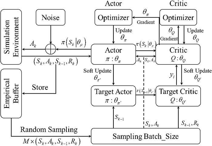
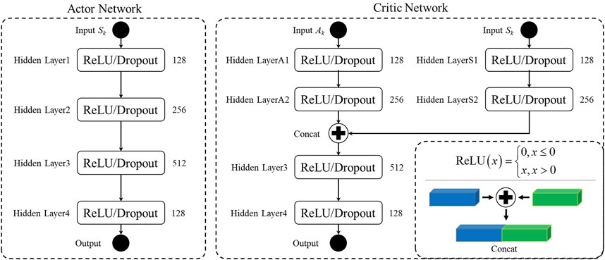
The DDPG model is an improvement of the deep Q-learning network and is combined with the idea of the deterministic policy gradient algorithm, which is a model-free DRL algorithm. The Actor-Critic (AC) architecture is applied to the DDPG model as its algorithm basic framework (Gopalakrishnan et al., 2016). Moreover, neural network is introduced as the approximation of its policy network and value network. The DDPG algorithm structure is shown in Figure 2.

Figure 2

Figure 2. Diagram of the DDPG model structure.

Each part of the AC architecture for the DDPG model uses two neural-network structures to form four neural networks in total, that is, the Actor network, Target Actor network, Critic network, and target Critic network. The Actor network is used for executing the policy, and the Critic network is used to evaluate the executed policy. Additionally, the DDPG model adopts deterministic policy gradient to update the model parameters. In the process of training, the Actor network calculate an action according to current state $S_k$ based on $\pi (S_k|{\theta }_{\mu })$. The Gaussian noise is added into the generated action $A_k$ to sufficiently explore the simulation environment. Subsequently, action $A_k$ is input into the simulation environment to generate the next state $S_{k+1}$ and obtain the corresponding reward $R_k$. After a step, current state $S_k$, action $A_k$, next state $S_k+1$, and reward $R_k$ are combined to form a quadruple ($S_k$, $A_k$, $S_k+1$, $R_k$) and stored in the empirical buffer for batch training of the model.

After $Nu$ samples of the Actor network training, the $M$ samples, that is, the quadruple ($S_k$, $A_k$, $S_{k+1}$, $R_k$) are randomly obtained from the empirical buffer to calculate target $y_i$ with discount rate $\gamma$ and each Critic network loss function. The calculation is expressed as Equation 24:

$\left\{\begin{array}{c}{y}_i=R_i+\gamma \min Q\left({S^{\prime }}_i,{A^{\prime }}_i\left|{\theta }_{Q^{\prime }}\right.\right)\hfill \\ {A^{\prime }}_i={\pi }_c\left({S^{\prime }}_i\left|{\theta }_{{\pi }^{\prime }}\right.\right)\hfill \\ L_Q\left({\theta }_Q\right)=\frac{1}{M}{\displaystyle \sum _{i=1}^M}{\left(y_i-Q\left(S_i,A_i\left|{\theta }_Q\right.\right)\right)}^2\hfill \\ i=\mathrm{1,2},\dots ,M\hfill \end{array}\right.(24)$

The parameter ${\theta }_{\pi }$ in the policy network is updated through the policy gradient based on the $M$ samples. The update goal is to maximize the Q network critic value as follows:

$\begin{array}{c}{\mathrm{\nabla }}_{{\theta }_{\pi }}J\left({\theta }_{\pi }\right)=\frac{1}{M}{\displaystyle \sum _{i=1}^M}{\mathrm{\nabla }}_{A}Q\left(S_i,A\left|{\theta }_Q\right.\right){|}_{A={\pi }_c\left(S_i\left|{\theta }_{\pi }\right.\right)}\hfill \\ {\mathrm{\nabla }}_{{\theta }_{\pi }}{\pi }_c\left(S_i\left|{\theta }_{\pi }\right.\right)\hfill \end{array}(25)$

where ${\pi }_c(S_i^{\prime }|{\theta }_{{\pi }^{\prime }})$ represents the Target Actor network; $Q(S_i,A|{\theta }_Q)$ represents the Target Critic network. The Target Actor network has the same network structure as the Actor network, and the Target Critic network has the same network structure as the Critic network. The Actor network and the Critic network structures are shown in Figure 3.

Figure 3

Figure 3. Structure of the Actor network and the Critic network based on DDPG.

The model parameters are updated using the soft update strategy as follows:

${\theta }_{Q^{\prime }}\leftarrow \tau {\theta }_Q+\left(1-\tau \right){\theta }_{Q^{\prime }}(26)$

${\theta }_{{\pi }^{\prime }}\leftarrow \tau {\theta }_{\pi }+\left(1-\tau \right){\theta }_{{\pi }^{\prime }}(27)$

where $\tau$ represents the momentum of the model parameter update, $\tau \in [\mathrm{0,1}]$, which is set to 0.005 in this study. The training of the DRL-based agent based on DDPG is depicted as Algorithm 1.

Algorithm 1

Algorithm 1. Training process of DDPG for line-parameter identification.

3.2 Line-aging assessment based on the line-parameter identification

Actual line parameters are identified using the proposed DDPG model. However, line aging seriously affects the transmission quality of power systems. Therefore, line aging should be roughly estimated based on line-parameter identification results. The line-aging indexes, namely ${\omega }_R^i$ and ${\omega }_X^i$, are expressed by calculating the degree of deviation of identified line parameters from theoretical line parameters according to Equation 28:

$\left\{\begin{array}{c}{\omega }_R^i=\left|{\widehat{\theta }}_R^i-{\theta }_R^{\mathit{true,i}}\right|/{\theta }_R^{\mathit{true,i}}\hfill \\ {\omega }_X^i=\left|{\widehat{\theta }}_X^i-{\theta }_X^{\mathit{true,i}}\right|/{\theta }_X^{\mathit{true,i}}\hfill \end{array}\right.(28)$

where ${\theta }_R^{\mathit{true,i}}$ and ${\theta }_X^{\mathit{true,i}}$ represent the standard resistance and reactance parameters of the $i$-th line, respectively. These parameters are set according to the factory specifications of the line.

The line-aging risk level of each line is calculated as the sum of ${\omega }_R^i$ and ${\omega }_X^i$ over a period of time, as follows:

$A_i=\frac{1}{T}{\displaystyle \sum _{t=1}^T}\left({\omega }_{R,t}^i+{\omega }_{X,t}^i\right)(29)$

4 Case studies

4.1 Case description and experimental setup

In this section, the proposed DDPG-based model performance is validated on IEEE 14-node and IEEE 33-node test systems. Details regarding the two test systems are as follows:

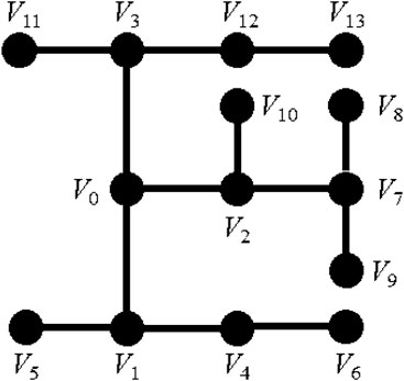
Case 1: The modified IEEE 14-node medium-voltage distribution system is used as the basic case, named IEEE14-M. IEEE14-M (shown in Figure 4) is a 23 kV medium-voltage distribution system, with 14 nodes and 13 transmission lines. The datas of each node, that is, the nodal active power, reactive power, and voltage magnitude, is simulated using the pandapower Python package (Thurner et al., 2018) to simulate the measurement data collected by SCADA. The numerical nodal injected active powers are generated using the Monte Carlo method in the range of [0.8$P_s$, 1.2$P_s$], where $P_s$ represents the standard active power of each node, and the reactive power $Q_s$ is calculated using the power factor. In practice, the power factor is between 0.8 and 0.95. The corresponding nodal voltage is obtained by executing power-flow function of the pandapower.

Figure 4

Figure 4. IEEE14-M medium-voltage distribution system.

Case 2: The IEEE 33-node medium-voltage distribution system is defined as IEEE33. The IEEE33 is a 12.66 kV distribution system, with 32 transmission lines (Zhao et al., 2020). The simulated measurement data are generated in the same manner as IEEE14-M.

All experiments are performed on a computer with i1-9700 @3.00 GHz CPU, 64 RAM, and GeForce GTX 1080Ti GPU. In addition, the software environment configuration is Python v3.10, Pytorch v2.1.0-cuda, and pandapower v2.11.0. A total of 10,000 episodes is carried out.

To demonstrate the performance of the proposed DDPG model, the DDPG model is compared with the proximal policy optimization (PPO) algorithm, soft actor-critic (SAC) algorithm and the weighted least square (WLS) algorithm, a classical method of parameter identification. In the DDPG model, the agent makes decision with Gaussian noise, which has a standard deviation 0.01. The learning rates of the Actor network and the Critic network are 0.002 and 0.001, respectively (Gopalakrishnan et al., 2016). The discount rate $\gamma$ is set to 0.9. The batch size is 32. The observation deviation reflects the gap between the model output and the real observation, which directly affects the accuracy of parameter identification. The observation deviation reward weights ${\lambda }_o$ is set to 0.6 to highlight that the model needs to reduce the observation deviation as the main optimization direction and ensure that the identified parameters can accurately reflect the actual system state. In addition, the parameter state reward and action reward are to encourage the model to gradually adjust and optimize toward the correct parameter state, avoiding frequent and unreasonable adjustments. Therefore, the corresponding reward weights, ${\lambda }_{\theta }$ and ${\lambda }_a$, are set to 0.2 to balance the exploration of suitable sitting and the maintenance of stable output. In the PPO model, the training process is set as previously described (Schulman et al., 2017).

4.2 Training performance

Reward values can provide a rough estimate of the line-parameter fitting accuracy. According to Equation 19, it can be seen that the calculation results identified using line parameters is closer to the measurement data, and the reward value is smaller. This means that, when the reward value is close to 0, the line-parameter identification accuracy is better. Figure 5 (red line) presents the average reward curve for the DDPG model in training. It can be seen that the DDPG can exhibit fast convergence, and the reward value is −0.31 at the end-step, showing that the correction strategy can reduce the simulated observation error corresponding to the correction parameter to the parameter observation error level. Additionally, the reward curve of the DDPG model is stable during training process owing to the AC strategy and the state design. Figure 5 (blue line) shows the average reward curve during the PPO training. As can be seen from Figure 5, the convergence and stability of the PPO algorithm are inferior to those of the DDPG model, and the final reward is −0.92. This is primarily due to the lower sampling efficiency of the PPO algorithm during policy training, leading to less accurate parameter identification than the DDPG model. Figure 5 (green line) shows the average reward curve during the SAC trining. It can be seen that the convergence of SAC is more stable, but the convergence speed is slow, and the final identification reward is −0.98. In general, compared with the SAC model, the PPO model converges faster in line-parameter identification, but the effect is unstable. However, the DDPG model not only shows higher stability in the training process, but also achieves significantly better final reward value. The results show that the DDPG model can more accurately realize the parameter adjustment and optimization strategy of distribution network line-parameter identification.

Figure 5

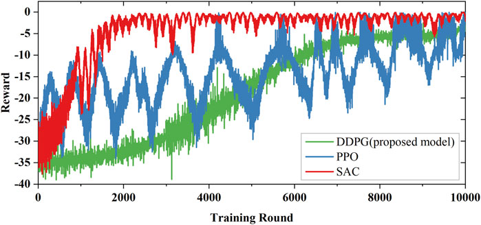
Figure 5. Average reward during training in IEEE14-M: red line is DDPG model training; blue line is PPO model training.

4.3 Test performance

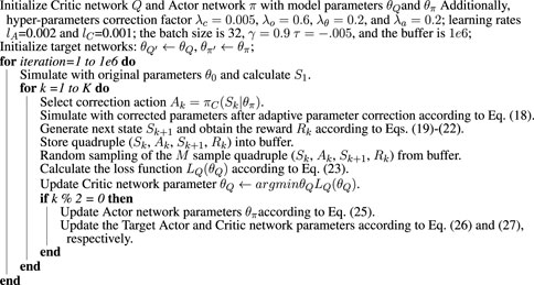
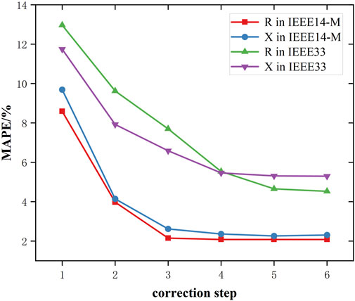
After the training is completed (the proposed DDPG model in Algorithm 1), the medium-voltage distribution network line-parameter identification strategy are loaded into the online strategy to realize the online line-parameter identification, and the test is carried out in 100 test scenarios. Subsequently, for all 100 test scenarios, the MAPE of the observed values are calculated at each step corresponding to the typical parameters, as shown in Figure 6. After the first correction, the average MAPE decreases by 59.16% for IEEE14-M and 39.59% for IEEE33. In addition, For the IEEE14-M system, the MAPE of parameters R and X decreases to 2.08% and 2.36% after averaging three steps of correction, respectively. For the IEEE33 system, the MAPE of parameters R and X decreases to 4.65% and 5.31% after averaging five steps of correction, respectively. It indicates that the corrective action of the line parameter identification strategy is basically completed. It can be seen that in the online implementation, appropriate identification parameters can be obtained by averaging 3 correction steps for the IEEE14-M system and 5 correction steps for the IEEE33 system.

Figure 6

Figure 6. Observation MAPE results of different correction steps.

4.4 Case 1 line-parameter identification and line-aging assessment

The proposed DDPG model can effectively identify the parameters of IEEE14-M lines, shown in Figure 7 When nodal voltage magnitude $V_i$ contains 1% Gaussian noise during the simulation of measurement data, the deviation of the 7-th line (from the 2-nd bus to 7-th bus) in the $R$ identification results is largest shown as Figure 5, and the deviation is 3.82%. The first line (from 0-th bus to 1-st bus) has the largest deviation from the actual value of line reactance, and the deviation is 4.37%. Combined with Figure 5, it can be seen that the voltage magnitude deviation of 2-nd bus is the largest, which is caused by the deviation of the $X$ parameter identification result of the first line. However, the measurement of voltage magnitude has 1% Gaussian noise. Moreover, part of the action design adds Gaussian noise with $s$ = 0.02, so that there is a certain deviation when fitting the objective function. The deviation of the voltage magnitude is 0.39%, which is within the acceptable range. Additionally, Figure 5 shows the identification deviation of the line parameters, that is, $R$, and $X$, which showed values of 2.244% and 2.372% compared with actual line parameters at single time slice. This demonstrates that the proposed DDPG model is effective in the case of a large difference degree of line parameters. Moreover, the parameter adaptive correction and Max-Min-Norm can effectively suppress the influence of the difference degree.

Figure 7

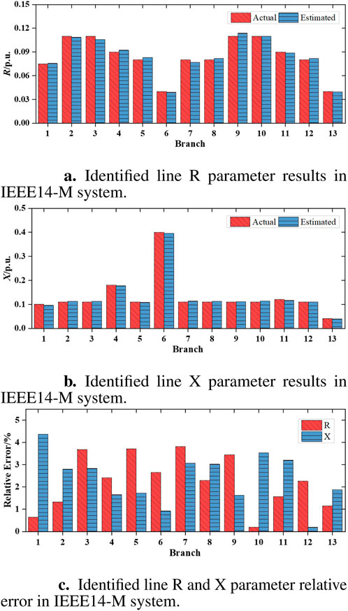
Figure 7. Line R and X parameter identification results and relative error in IEEE14-M system. (A) Identified line R parameter results. (B) Identified line X parameter results. (C) Identified line R and X parameter relative error.

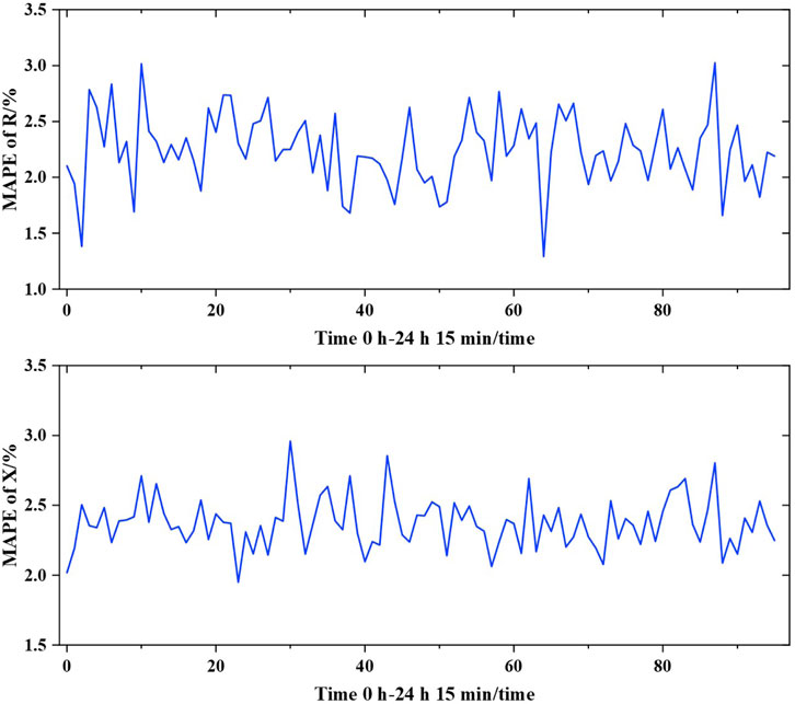
Since the nodal injected power of each node changes with time, single identification results are not sufficient to reflect the identification accuracy. Therefore, multi-temporal cross-section experiments are conducted using the proposed DDPG model from 01:00 to 00:00. In this study, pandapower is used for simulating the measurement data collected by SCADA within 1 day, and the sampling frequency is 15min/time. A period of measurement data are input into the proposed model for sequence verification, and the errors of the $R$ and $X$ over a period of time are shown in Figure 8. The line parameters $R$ and $X$’s mean absolute percentage error (MAPE) are 2.45% and 2.52% respectively, for all lines records. This low error rate highlights the model’s robustness in handling dynamic conditions, where injected power fluctuates throughout the day. A key advantage of the DDPG model is its capacity for real-time adaptation, providing consistent accuracy across various time slices. The model’s ability to capture these temporal variations ensures a high level of precision in parameter identification, even under changing system dynamics. This makes it particularly suitable for practical distribution network applications, where operational conditions are in constant flux. Furthermore, the high identification accuracy allows distribution network operators to rely on the model for continuous system monitoring and aging assessment, ensuring system stability and reliability. This demonstrates the model’s advantage in providing accurate, real-time parameter estimation with low computational complexity.

Figure 8

Figure 8. Line R and X parameter identification MAPE during a period of time.

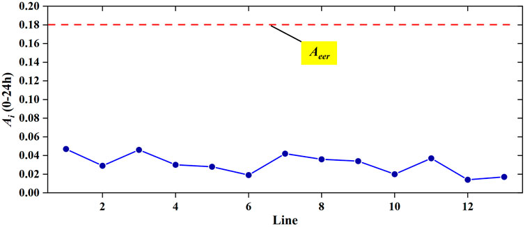
The result of the line-aging assessment is shown in Figure 9. Usually, according to the actual situation, a distribution-network operator can set the aging warning coefficient $A_{\mathit{err}}$. According to Wu et al. (2022), the $V_{\mathit{err}}$ is set to 0.18, and as presented in Figure 8, all lines in the IEEE14-M are in the normal state. It should be noted that the line-aging risk level of each line is calculated over a period of time, according to Equation 29.

Figure 9

Figure 9. Results of line aging assessment of IEEE14-M.

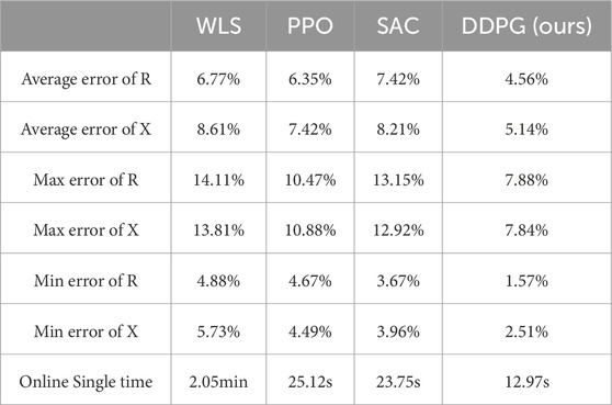
In order to verify the performance of the proposed method, the proposed DDPG model is compared with WLS, SAC and PPO model. Table 1 summarizes the results for different algorithms. The average identification deviation of line parameters R and X under the WLS, SAC and PPO method are 5.8% (WLS-R), 7.12% (WLS-X), 6.12% (SAC-R), 6.54% (SAC-X), 4.2% (PPO-R) and 5.44% (PPO-X). The identification accuracy of the proposed DDPG method is better than that of the other methods. This underlines the superior performance and accuracy of the proposed DDPG model in line-parameter identification and aging assessment tasks. The superior performance of the DDPG model stems from its actor-critic structure, which enables efficient and stable policy updates, and its ability to handle continuous action spaces, providing precise control over line parameters in medium-voltage systems. Compared to PPO and SAC model, DDPG model offers better sample efficiency and focused optimization, reducing parameter deviation. Its deterministic policy gradient minimizes errors between observed and predicted parameters, while noise injection ensures stable exploration. Additionally, the DDPG model demonstrates a lower computational time complexity, requiring less time to converge compared to SAC, making it more suitable for real-time applications. These factors make DDPG more accurate and stable for real-time line-parameter identification and aging assessments, with lower computational overhead, ideal for distribution networks.

Table 1

Table 1. Summary of identification with different methods.

4.5 Case 2 line-parameter identification and line-aging assessment

In the test case, the line parameters of the IEEE33 medium-voltage distribution system are identified using the proposed DDPG model. The test is based on the same sampling frequency, that is, 15-min. Similarly, a 1% Gaussian noise is added to the measurement data $\left(V_i\right)$. The identification results are shown in Figure 10. It can be seen that the proposed DDPG method can exactly identify the line parameters of each branch, namely $R$ (shown as Figure 5) and $X$ (shown as Figure 5). Moreover, the corresponding average relative errors are 4.56% and 5.15%, respectively. It is reflected in both cases that the deviation of the line resistance identification results is smaller compared with that of the line reactance. If the possible measurement error is taken into account, the identification results meet the requirement. The minimum identification error of line parameters, $R$ and $X$, as shown in Figure 5 are 1.56% and 2.51% respectively, and the corresponding maximum identification errors are 7.88% and 7.83%, respectively. The results indicate that the identification of line resistance tends to be more accurate than that of line reactance, and all identification errors fall within acceptable ranges, demonstrating the model’s robustness to measurement errors.

Figure 10

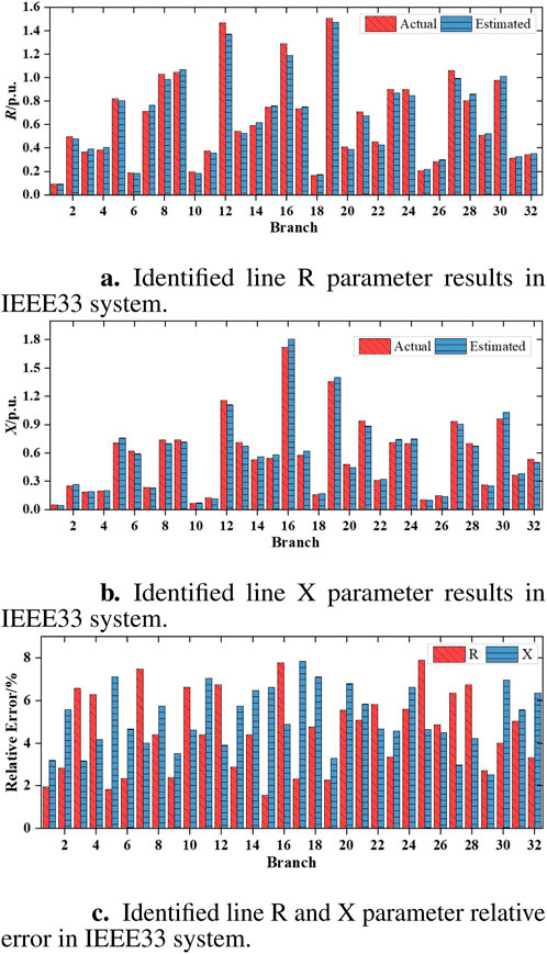
Figure 10. Line R and X parameter identification results and relative error in IEEE33 system. (A) Identified line R parameter results. (B) Identified line X parameter results. (C) Identified line R and X parameter relative error.

In order to sufficiently reflect the identification accuracy, multi-temporal cross-section experiments are conducted within 1 day from 01:00 to 00:00. Similar to Case 1, pandapower is used to simulating the SCADA measurement data and the sampling frequency is also 15-min/time. The errors of $R$ and $X$ over a period of time are shown in Figure 11. The MAPEs of line parameters $R$ and $X$ are 4.72% and 5.45%, respectively, for all lines records. And the stability and reliability of the proposed DDPG model over time in a dynamic operating environment. This demonstrates that the identification result accuracy is independent of the nodal injection power fluctuation over a period of time (from 01:00 to 00:00 of a day). This consistency in accuracy, regardless of nodal injection power fluctuations, highlights the DDPG model’s resilience and stability in a real-world operating environment. Unlike traditional methods, the DDPG algorithm excels in environments with temporal variability, maintaining its precision across different time slices and system conditions. The model’s robustness ensures it is well-suited for dynamic distribution networks, where power flow and operational conditions continuously change. This high level of adaptability makes it a reliable tool for real-time monitoring and line-parameter identification in practical applications, offering operators confidence in its stability over time. The relatively low computational complexity also makes it feasible for deployment in large-scale systems, where speed and accuracy are critical.

Figure 11

Figure 11. Line $R$ and $X$ parameter identification MAPE of IEEE33 system during a period of time.

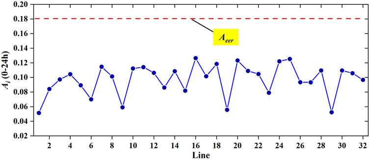
The result of line-aging assessment of IEEE33 system is shown in Figure 12. The line parameters in the IEEE33 system are maintained at normal level, but they are very close to the aging warning coefficient $A_{\mathit{eer}}$ (set to 0.18 in 4.3). Regarding the lines parameter identification results of the IEEE33 system, the lines close to the aging warning coefficient are the 16-th, 20-th, 24-th, and 25-th line, and the $A_i$ of the above lines exceeds 0.12. The average aging risk level of all lines in the IEEE33 system is 0.097, and all lines are in the normal state at present.

Figure 12

Figure 12. Result of line aging assessment of IEEE33 system.

The proposed DDPG model is compared with WLS, SAC and PPO algorithms to verify the effectiveness of DDPG, and the comparison results are shown in Table 2. The average identification deviation of line parameters R and X under the different methods are 6.77% (WLS-R), 8.61% (WLS-X), 6.35% (PPO-R), 7.42% (PPO-X), 7.42% (SAC-R), 8.21% (SAC-X), 4.56% (DDPG-R ours), and 5.14% (DDPG-X ours), respectively. This superior performance is due to DDPG’s efficient policy optimization and ability to operate in continuous action spaces, ensuring better accuracy in parameter identification, even in noisy conditions. In terms of computational complexity, although computationally more intensive than WLS or PPO model, ensures better convergence and stability. On average, DDPG completes parameter identification for the IEEE33 system within 12.97 s, faster than SAC (23.75 s) due to DDPG’s deterministic policy updates and more focused exploration. This makes DDPG well-suited for real-time applications in large-scale modern smart grid application.

Table 2

Table 2. Summary of identification with different methods.

5 Conclusion

Accurate identification of line parameters in distribution systems is crucial for improving their security and reliability, given their direct connection to end-users. This study proposes a DDPG-based method for line-parameter identification in medium-voltage distribution systems, validated on IEEE14-M and IEEE33 systems. By transforming the problem into a MDP and constructing an agent with a fitting objective function, the proposed method provides a novel approach compared to traditional methods. The results show that the DDPG method achieves lower identification deviations—2.24% and 2.37% in IEEE14-M, and 4.56% and 5.14% in IEEE33 compared to the WLS and PPO methods. Additionally, the DDPG approach only requires nodal measurements of injected active power, reactive power, and voltage magnitude, simplifying the process without sacrificing accuracy. With advancements in smart grids, data-driven deep learning methods will further enhance parameter identification for distribution systems. Future research will focus on extending this method to broader line parameters, addressing challenges like limited sample data and adaptive topology.

Data availability statement

The raw data supporting the conclusions of this article will be made available by the authors, without undue reservation.

Author contributions

XJ: Formal Analysis, Methodology, Resources, Writing–original draft. LF: Conceptualization, Resources, Visualization, Writing–original draft. CZ: Software, Validation, Writing–original draft. KC: Data curation, Investigation, Writing–review and editing. YX: Project administration, Writing–review and editing. BW: Supervision, Writing–review and editing.

Funding

The author(s) declare financial support was received for the research, authorship, and/or publication of this article. $•$ Science and Technology Project of State Grid Corporation (No. J2023018).

Conflict of interest

Authors XJ, LF, CZ, KC, YX and BW were employed by State Grid Jiangsu Electric Power Co., Ltd.

Publisher’s note

All claims expressed in this article are solely those of the authors and do not necessarily represent those of their affiliated organizations, or those of the publisher, the editors and the reviewers. Any product that may be evaluated in this article, or claim that may be made by its manufacturer, is not guaranteed or endorsed by the publisher.

References

Chang, C., Tao, C., Wang, S., Zhang, R., Tian, A., and Jiang, J. (2023). A fault diagnosis method for lithium batteries based on optimal variational modal decomposition and dimensionless feature parameters. J. Electrochem. Energy Convers. Storage 20, 031004. doi:10.1115/1.4055536

CrossRef Full Text | Google Scholar

Dutta, R., Patel, V. S., Chakrabarti, S., Sharma, A., Das, R. K., and Mondal, S. (2021). Parameter estimation of distribution lines using scada measurements. IEEE Trans. Instrum. Meas. 70, 1–11. doi:10.1109/TIM.2020.3026116

PubMed Abstract | CrossRef Full Text | Google Scholar

Glavic, M. (2019). (deep) reinforcement learning for electric power system control and related problems: a short review and perspectives. Annu. Rev. Control 48, 22–35. doi:10.1016/j.arcontrol.2019.09.008

CrossRef Full Text | Google Scholar

Gogula, V., and Edward, B. (2023). Fault detection in a distribution network using a combination of a discrete wavelet transform and a neural network’s radial basis function algorithm to detect high-impedance faults. Front. Energy Res. 11, 1101049. doi:10.3389/fenrg.2023.1101049

CrossRef Full Text | Google Scholar

Gopalakrishnan, R., Goutam, S., Miguel Oliveira, L., Timmermans, J.-M., Omar, N., Messagie, M., et al. (2016). A comprehensive study on rechargeable energy storage technologies. J. Electrochem. Energy Convers. Storage 13, 040801. doi:10.1115/1.4036000

CrossRef Full Text | Google Scholar

Hu, J., Wang, Q., Ye, Y., and Tang, Y. (2023). Toward online power system model identification: a deep reinforcement learning approach. IEEE Trans. Power Syst. 38, 2580–2593. doi:10.1109/TPWRS.2022.3180415

CrossRef Full Text | Google Scholar

Kumar, N. (2024). Ev charging adapter to operate with isolated pillar top solar panels in remote locations. IEEE Trans. Energy Convers. 39, 29–36. doi:10.1109/tec.2023.3298817

CrossRef Full Text | Google Scholar

Kumar, N., Mulo, T., and Verma, V. P. (2013). “Application of computer and modern automation system for protection and optimum use of high voltage power transformer,” in 2013 international conference on computer communication and informatics, Coimbatore, India, 04-06 January 2013 (IEEE) 1–5.

CrossRef Full Text | Google Scholar

Kumar, N., Panigrahi, B. K., and Singh, B. (2016). A solution to the ramp rate and prohibited operating zone constrained unit commitment by ghs-jgt evolutionary algorithm. Int. J. Electr. Power and Energy Syst. 81, 193–203. doi:10.1016/j.ijepes.2016.02.024

CrossRef Full Text | Google Scholar

Kumar, N., Saxena, V., Singh, B., and Panigrahi, B. K. (2020). Intuitive control technique for grid connected partially shaded solar pv-based distributed generating system. IET Renew. Power Gener. 14, 600–607. doi:10.1049/iet-rpg.2018.6034

CrossRef Full Text | Google Scholar

Kumar, N., Saxena, V., Singh, B., and Panigrahi, B. K. (2023a). Power quality improved grid-interfaced pv-assisted onboard ev charging infrastructure for smart households consumers. IEEE Trans. Consumer Electron. 69, 1091–1100. doi:10.1109/tce.2023.3296480

CrossRef Full Text | Google Scholar

Kumar, N., Singh, H. K., and Niwareeba, R. (2023b). Adaptive control technique for portable solar powered ev charging adapter to operate in remote location. IEEE Open J. Circuits Syst. 4, 115–125. doi:10.1109/ojcas.2023.3247573

CrossRef Full Text | Google Scholar

Lakshminarayana, S., Sthapit, S., and Maple, C. (2021). A comparison of data-driven techniques for power grid parameter estimation. arXiv. doi:10.48550/arXiv.2107.03762

CrossRef Full Text | Google Scholar

Li, F., and Du, Y. (2018). From alphago to power system ai: what engineers can learn from solving the most complex board game. IEEE Power Energy Mag. 16, 76–84. doi:10.1109/MPE.2017.2779554

CrossRef Full Text | Google Scholar

Li, H., Weng, Y., Vittal, V., and Blasch, E. (2024). Distribution grid topology and parameter estimation using deep-shallow neural network with physical consistency. IEEE Trans. Smart Grid 15, 655–666. doi:10.1109/TSG.2023.3278702

CrossRef Full Text | Google Scholar

Liu, W., Gao, S., and Yan, W. (2024). Comparison-transfer learning based state-of-health estimation for lithium-ion battery. J. Electrochem. Energy Convers. Storage 21, 1–34. doi:10.1115/1.4064656

CrossRef Full Text | Google Scholar

Loshchilov, I., and Hutter, F. (2019). Decoupled weight decay regularization. arXiv. https://arxiv.org/abs/1711.05101.

Google Scholar

Ma, L., Wu, L., Liu, N., and Pei, W. (2022). A two-step approach for multi-topology identification and parameter estimation of power distribution networks. CSEE J. Power Energy Syst., 1–10doi. doi:10.17775/CSEEJPES.2021.08180

CrossRef Full Text | Google Scholar

Pegoraro, P. A., Brady, K., Castello, P., Muscas, C., and von Meier, A. (2019). Line impedance estimation based on synchrophasor measurements for power distribution systems. IEEE Trans. Instrum. Meas. 68, 1002–1013. doi:10.1109/TIM.2018.2861058

CrossRef Full Text | Google Scholar

Recht, B. (2019). A tour of reinforcement learning: the view from continuous control. Annu. Rev. Control, Robotics, Aut. Syst. 2, 253–279. doi:10.1146/annurev-control-053018-023825

CrossRef Full Text | Google Scholar

Satapathy, S. S., and Kumar, N. (2019). “Modulated perturb and observe maximum power point tracking algorithm for solar pv energy conversion system,” in 2019 3rd international conference on recent developments in control, automation power engineering (RDCAPE), Noida, India, 10-11 October 2019, (IEEE) 345–350.

CrossRef Full Text | Google Scholar

Schulman, J., Wolski, F., Dhariwal, P., Radford, A., and Klimov, O. (2017). Proximal policy optimization algorithms. arXiv. https://arxiv.org/abs/1707.06347

Google Scholar

Srinivas, V. L., and Wu, J. (2022). Topology and parameter identification of distribution network using smart meter and µPMU measurements. IEEE Trans. Instrum. Meas. 71, 1–14. doi:10.1109/TIM.2022.3175043

CrossRef Full Text | Google Scholar

Sukanya Satapathy, S., and Kumar, N. (2020). Framework of maximum power point tracking for solar pv panel using wsps technique. IET Renew. Power Gener. 14, 1668–1676. doi:10.1049/iet-rpg.2019.1132

CrossRef Full Text | Google Scholar

Sun, J., Chen, Q., and Xia, M. (2024). Data-driven detection and identification of line parameters with pmu and unsynchronized scada measurements in distribution grids. CSEE J. Power Energy Syst. 10, 261–271. doi:10.17775/CSEEJPES.2020.06860

CrossRef Full Text | Google Scholar

Sun, J., Xia, M., and Chen, Q. (2019). A classification identification method based on phasor measurement for distribution line parameter identification under insufficient measurements conditions. IEEE Access 7, 158732–158743. doi:10.1109/ACCESS.2019.2950461

CrossRef Full Text | Google Scholar

Sun, X., and Qiu, J. (2021). Two-stage volt/var control in active distribution networks with multi-agent deep reinforcement learning method. IEEE Trans. Smart Grid 12, 2903–2912. doi:10.1109/TSG.2021.3052998

CrossRef Full Text | Google Scholar

Thurner, L., Scheidler, A., Schäfer, F., Menke, J.-H., Dollichon, J., Meier, F., et al. (2018). Pandapower—an open-source python tool for convenient modeling, analysis, and optimization of electric power systems. IEEE Trans. Power Syst. 33, 6510–6521. doi:10.1109/TPWRS.2018.2829021

CrossRef Full Text | Google Scholar

Wang, W., and Yu, N. (2022). Estimate three-phase distribution line parameters with physics-informed graphical learning method. IEEE Trans. Power Syst. 37, 3577–3591. doi:10.1109/TPWRS.2021.3134952

CrossRef Full Text | Google Scholar

Wang, X., Wang, Y., Shi, D., Wang, J., and Wang, Z. (2020). Two-stage wecc composite load modeling: a double deep q-learning networks approach. IEEE Trans. Smart Grid 11, 4331–4344. doi:10.1109/TSG.2020.2988171

CrossRef Full Text | Google Scholar

Wang, X., Zhao, Y., and Zhou, Y. (2024). A data-driven topology and parameter joint estimation method in non-pmu distribution networks. IEEE Trans. Power Syst. 39, 1681–1692. doi:10.1109/TPWRS.2023.3242458

CrossRef Full Text | Google Scholar

Wang, Y., Xia, M., Yang, Q., Song, Y., Chen, Q., and Chen, Y. (2022). Augmented state estimation of line parameters in active power distribution systems with phasor measurement units. IEEE Trans. Power Deliv. 37, 3835–3845. doi:10.1109/TPWRD.2021.3138165

CrossRef Full Text | Google Scholar

Wu, Z., Long, H., and Chen, C. (2022). Line aging assessment in distribution network based on topology verification and parameter estimation. J. Mod. Power Syst. Clean Energy 10, 1658–1668. doi:10.35833/MPCE.2021.000165

CrossRef Full Text | Google Scholar

Xie, J., Ma, Z., Dehghanpour, K., Wang, Z., Wang, Y., Diao, R., et al. (2021). Imitation and transfer q-learning-based parameter identification for composite load modeling. IEEE Trans. Smart Grid 12, 1674–1684. doi:10.1109/TSG.2020.3025509

CrossRef Full Text | Google Scholar

Yan, Z., and Xu, Y. (2020). Real-time optimal power flow: a Lagrangian based deep reinforcement learning approach. IEEE Trans. Power Syst. 35, 3270–3273. doi:10.1109/TPWRS.2020.2987292

CrossRef Full Text | Google Scholar

Yang, N.-C., Huang, R., and Guo, M.-F. (2022). Distribution feeder parameter estimation without synchronized phasor measurement by using radial basis function neural networks and multi-run optimization method. IEEE Access 10, 2869–2879. doi:10.1109/ACCESS.2021.3140123

CrossRef Full Text | Google Scholar

Yu, J., Weng, Y., and Rajagopal, R. (2018). Patopa: a data-driven parameter and topology joint estimation framework in distribution grids. IEEE Trans. Power Syst. 33, 4335–4347. doi:10.1109/TPWRS.2017.2778194

CrossRef Full Text | Google Scholar

Yu, X., Fernando, B., Hartley, R., and Porikli, F. (2020). Semantic face hallucination: super-resolving very low-resolution face images with supplementary attributes. IEEE Trans. Pattern Analysis Mach. Intell. 42, 2926–2943. doi:10.1109/TPAMI.2019.2916881

CrossRef Full Text | Google Scholar

Zhang, J., Wang, P., and Zhang, N. (2021). Distribution network admittance matrix estimation with linear regression. IEEE Trans. Power Syst. 36, 4896–4899. doi:10.1109/TPWRS.2021.3090250

CrossRef Full Text | Google Scholar

Zhang, J., Wang, Y., Weng, Y., and Zhang, N. (2020). Topology identification and line parameter estimation for non-pmu distribution network: a numerical method. IEEE Trans. Smart Grid 11, 4440–4453. doi:10.1109/TSG.2020.2979368

CrossRef Full Text | Google Scholar

Zhao, J., Li, L., Xu, Z., Wang, X., Wang, H., and Shao, X. (2020). Full-scale distribution system topology identification using markov random field. IEEE Trans. Smart Grid 11, 4714–4726. doi:10.1109/tsg.2020.2995164

CrossRef Full Text | Google Scholar

Zhou, Q., Wang, C., Sun, Z., Li, J., Williams, H., and Xu, H. (2021). Human-knowledge-augmented Gaussian process regression for state-of-health prediction of lithium-ion batteries with charging curves. J. Electrochem. Energy Convers. Storage 18, 030907. doi:10.1115/1.4050798

CrossRef Full Text | Google Scholar

Zhou, X., Wang, S., Diao, R., Bian, D., Duan, J., and Shi, D. (2020). Rethink ai-based power grid control: diving into algorithm design. arXiv.

Google Scholar