Electricity consumption forecasting using a novel homogeneous and heterogeneous ensemble learning

In today’s world, a country’s economy is one of the most crucial foundations. However, industries’ financial operations depend on their ability to meet their electricity demands. Thus, forecasting electricity consumption is vital for properly planning and managing energy resources. In this context, a new approach based on ensemble learning has been developed to predict monthly electricity consumption. The method divides electricity consumption time series into deterministic and stochastic components. The deterministic component, which consists of a secular long-term trend and an annual seasonality, is estimated using a multiple regression model. In contrast, the stochastic part considers the short-run random fluctuations of the consumption time series. It is forecasted by four different time series, four machine learning models, and three novel proposed ensemble models: the time series homogeneous ensemble model, the machine learning ensemble model, and the heterogeneous ensemble model. The study analyzed data on Pakistan’s monthly electricity consumption from 1991-January to 2022-December. The evaluation of the forecasting models is based on three criteria: accuracy metrics (including the mean absolute percent error (MAPE), the mean absolute error (MAE), the root mean squared error (RMSE), and the root relative squared error (RRSE)); an equality forecast statistical test (the Diebold and Mariano’s test); and a graphical assessment. The heterogeneous ensemble model’s forecasting results show lower error values compared to the homogeneous ensemble models and the singles models, with accuracy metrics measured by MAPE, MAE, RMSE, and RRSE at 5.0027, 460.4800, 614.5276, and 0.2933, respectively. Additionally, the heterogeneous ensemble model is statistically significant (p $<$ 0.05) and superior to the rest of the models. Also, the heterogeneous ensemble model demonstrates considerable performance with the least mean error, which is comparatively better than the individual and best models reported in the literature and are considered baseline models. Further, the forecast values’ monthly behavior depicts that electricity consumption is higher during the summer season, and this demand will be highest in June and July. The forecast model and graph reveal that electricity consumption rapidly increases with time. This indirectly indicates that the government of Pakistan must take adequate steps to improve electricity production through different energy sources to restore the country’s economic status by meeting the country’s electricity demand. Despite several studies conducted from various perspectives, no analysis has been undertaken using an ensemble learning approach to forecast monthly electricity consumption for Pakistan.

1 Introduction

Electricity cannot be efficiently stored. Thus, it must be utilized as it is generated. As a result, it is critical to use only what is necessary. The distribution subsidiary orders electricity from the generating subsidiary and then delivers it to clients. Overproduction, or energy created but not delivered, is deemed a dead loss by the corporation. Thus, a greater forecast of consumer demand lowers mistakes in manufacturing orders, minimizing losses due to overproduction (Hu et al., 2024; Iftikhar, 2018; Wang et al., 2024; Hou et al., 2017).

At the distribution subsidiary level, there are also electricity losses that can have a significant impact. Losses can be classified into two types: technical and nontechnical. Non-technical losses include meter failures, fraudulent customer conduct, and management problems (Shah et al., 2019; Li et al., 2021; Lei et al., 2023). Technical losses are caused by electrical networks and equipment. Electricity losses may be calculated by summing technical and non-technical losses (Iftikhar et al., 2024c; Shirkhani et al., 2023; Ju et al., 2022). As a result, power suppliers established a yearly piloting system with a monthly verification point to monitor losses and implement operational changes to maintain a normative loss rate. Accurate monthly customer projections are critical to preventing outcomes from deviating from expectations (Duan et al., 2023; Wang et al., 2017; Iftikhar et al., 2024a). Therefore, the proposed high-accuracy forecasting method aims to improve the electricity suppliers’ piloting system.

Monthly electricity consumption forecasting has been extensively studied over the last four decades. Researchers have developed various techniques to forecast monthly electricity consumption, broadly classified into four categories: statistical methods, machine learning models, decomposition-combination techniques, and hybrid approaches (Shah et al., 2022; Gonzales et al., 2024). Statistical models, such as autoregressive-based models, exponential-smoothing models, and linear and nonlinear regression methods, are simple mathematical functional forms that are easy to apply (Elsaraiti et al., 2021; Omogoroye et al., 2023; Krstev et al., 2023). For instance, a study Shah et al. (2020) conducted in Pakistan used a component-wise forecasting approach to predict electric power consumption 1 month in advance, dividing the data into the deterministic component and the stochastic component. To model and forecast the first component (the deterministic), linear (parametric) and nonlinear (nonparametric) regression methods were used, while the second component (the stochastic) was modeled by four various time series models. The study found that linear and nonlinear regression approaches had the highest accuracy and efficacy with the combination of the autoregressive moving average model. Similarly, a study (Hussain et al., 2016) utilized the Holt-Winter and the ARIMA time series models to model and analyze secondary data from 1980 to 2011 to forecast Pakistan’s total electric power consumption and its individual components. The findings indicated that the Holt-Winter time series model was the most appropriate for this forecasting analysis. Furthermore, the research work projected an increase in electric power consumption, leading to a wider gap between consumption and production. The research recommended several strategies to mitigate the demand-supply disparity and ensure a consistent supply of electric power to various sectors of the economy.

In contrast, machine learning algorithms address the most complex nonlinear time series forecasting problems (Pham et al., 2020; Khalil et al., 2022; Gonzalez-Briones et al., 2019; Meng et al., 2024). For example, in a study Leite Coelho da Silva et al. (2022) conducted in Brazil, various time-series and machine-learning forecasting models were applied to the industrial electricity consumption dataset to forecast 1 month ahead. The findings showed that the multi-layer perceptron model had the best forecasting performance compared to all the other competitor models. In the decomposition-combination technique, the original time series data is divided into sub-series to improve performance by creating a more reliable form (Iftikhar et al., 2023c; Carbo-Bustinza et al., 2023; Feng et al., 2024). For instance, a study Iftikhar et al. (2023d) analyzing monthly electricity consumption in Pakistan decomposed the original electric power consumption series into three new subsequent: a secular long-term trend sub-series, a seasonal sub-series, and a stochastic sub-series. When applied to Pakistan’s monthly electric power consumption dataset, which ranges from 1990 to 2020, the proposed framework provided highly accurate and efficient gains, outperforming benchmark approaches and improving the performance of the final aggregate model forecasts. On the other hand, many researchers have also introduced hybrid models by merging the specific features of two or more models to build new models (Fan et al., 2020; Ding et al., 2022; Iftikhar et al., 2024b; Hajirahimi and Khashei, 2023). For example, a study Pełka (2023) proposed a method for mid-term load forecasting using hybrid statistical models that employ input data representing a load time series’ normalized annual seasonal cycle with filtered trend and unified variance. The proposed approach avoids the need to understand the complex time series and has several advantages over an alternative method that does not involve forecasting coding variables. The proposal tested mid-term load forecasting issues for thirty-five European countries and outperformed predecessors Prophet, ETS, and ARIMA by about 13.7%, 17.4%, and 25% in the case of MAPE error. The author claims the proposal can be used for short-term electric power demand forecasting.

As seen in the previous works on Pakistan’s electricity consumption (Hussain et al., 2016; Shah et al., 2020; Yasmeen and Sharif, 2014; Iftikhar et al., 2023a). The researchers have done their effects to achieve an accurate and efficient monthly forecast of electric power consumption in Pakistan. They used different forecasting models and methods in this context. However, there is a research gap among these studies; there is no reachable available to model and forecast the electric power consumption for Pakistan using the ensemble learning approach. Specifically to investigate the ensemble-based technique in the context of component-based forecasting. Thus, this work proposes three novel ensemble models based on various time-series and machine-learning models to implement and boost the forecasting accuracy of monthly electricity consumption in Pakistan. To do this, the electricity consumption time series is separated into two parts: the deterministic and the stochastic. The deterministic component, which includes a secular long-term trend and yearly seasonality, is modeled and forecast by a multiple regression model. However, the stochastic part considers the short-run fluctuations of the consumption time series. To model and forecast the stochastic part using four time-series models, four machine-learning models, and three novel proposed ensemble models: the time-series homogeneous ensemble model, the machine-learning ensemble model, and the heterogeneous ensemble model. The trials gathered data on Pakistan’s monthly power usage from 1991-January to 2022-December.

However, in Pakistan, energy consumption does not often provide any inferential analysis to examine variations in prediction accuracy amongst the models under consideration. Thus, this research’s primary contribution is to investigate the ensemble-based technique in the context of component-based forecasting. Furthermore, the forecasting ability is assessed over 6 years, and the importance of variations in prediction accuracy is studied. In addition, the introduced ensemble learning can capture the deterministic properties (secular long-term trend and yearly seasonality) of the power consumption time series, resulting in improved forecasting accuracy.

On the other hand, the critical differences among the past studies on the electric consumption of Pakistan are the following: a) the estimation of the deterministic part was parametric and nonparametric regression models. Conversely, some authors directly treated the deterministic part in a single forecasting model. While the current work only uses the multiple regression model. b) The stochastic component was modeled using four single time series models. In contrast, the current research work uses eleven different forecasting models, such as four different time series, four machine learning models, and three novel proposed ensemble models: the time series homogeneous ensemble model, the machine learning ensemble model, and the heterogeneous ensemble model to model and forecast the stochastic components. In this sense, despite several studies conducted from different perspectives, no analysis has been undertaken using an ensemble learning approach to forecast monthly electricity consumption for Pakistan.

The rest of the paper is organized in the following manner: In Section 2, the proposed ensemble-based forecasting methodology and its general procedure are described. Section 3 demonstrates an empirical application of the proposed ensemble forecasting methodology using Pakistan’s monthly electricity consumption data. Section 4 is a comparative discussion about the best ensemble model of this work versus the best models available in the literature and some well-known baseline models. Finally, Section 5 concludes the paper with remarks and future research directions.

2 The general procedure of the developed ensemble learning

This section describes the proposed ensemble forecasting approach for one-month-ahead power consumption forecasts. The electric power consumption time series has complicated properties. These properties are expected to include a secular long-run trend, pronounced seasonality, high volatility, non-normality, and non-stationarity. For instance, see Figure 1A for the monthly electric power consumption time series from 1991-January to 2022-December surprised with long-run linear secular trend components. In addition, It can show an increasing secular trend component in the electric power consumption time series. Figure 1B shows yearly consumption data for the past 32 years (1991–2022), which shows a continuously increasing trend in electric power consumption till 2008, while a slight decline in 2009 and again increasing in the consumption of electric power and attained a peak in 2019. However, it can also be observed that during the 2020 years, there was lower consumption, which was the leading cause of the COVID-19 pandemic. Figure 1C shows the average monthly electricity consumption over the past 32 years; it is confirmed from this figure that the consumption of electric power is lower during January, February, and March, while moderate during April, November, and December. However, higher electric power consumption was observed during the summary winter (May, June, July, and August). In the same way, September and October have higher consumption than the other months without the summary months. Figure 1D illustrates the monthly consumption for three consecutive years and confirms an annual seasonal effect. Figure 1E for the autocorrelation plot of the original electric power consumption at sixty lags, and Figure 1F for the partial autocorrelation plot of original electric power at sixty lags. These figures clearly illustrate a discernible nonlinear long-run trend and an annual seasonality. Furthermore, non-normality and non-stationarity are also evident from these visual representations. Thus, adding these patterns into the predictive model considerably improves forecast accuracy. The power consumption time series is divided into deterministic and stochastic to do this. The deterministic component, which includes a secular long-term trend and yearly seasonality, is calculated by a multiple regression model. However, the stochastic portion considers the short-run random changes in the consumption time series. It is predicted by four distinct time series, four machine learning models, and three new suggested ensemble models: the time series homogeneous ensemble model, the machine learning ensemble model, and the heterogeneous ensemble model. After estimating both sections individually, the estimates of the deterministic and stochastic components are combined to provide the final projections.

Figure 1

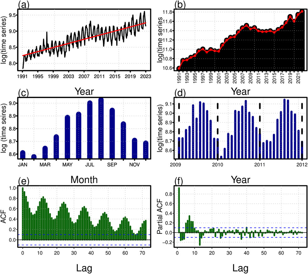
Figure 1. Characterization of Pakistan electric power consumption (kWh) (1991–2022): monthly electric power consumption time series plot (A); Yearly electric power consumption bar plot (B), displays average monthly electric power consumption over the past 32 years (C); monthly electric power consumption line plot for over the 3 years (D), autocorrelation function plot (E), partial autocorrelation function plot (F).

Let $(\text{log}({\mathfrak{E}}_{\mathfrak{n}}))$ be consumption time series of electric power for ${\text{n}}^{\text{th}}$ month. To model the features of the electric power consumption time series, the $(\text{log}({\mathfrak{E}}_{\mathfrak{n}}))$ might be as follows:

$\text{log}\left({\mathfrak{E}}_{\mathfrak{n}}\right)={\mathfrak{d}}_{\mathfrak{n}}+{\mathfrak{s}}_{\mathfrak{n}}(1)$

In the above Equation 1, the electric power consumption time series ${\mathfrak{E}}_{\mathfrak{n}}$ includes two significant components: ${\mathfrak{d}}_{\mathfrak{n}}$, which is deterministic, and ${\mathfrak{s}}_{\mathfrak{n}}$, which is stochastic. The deterministic component comprises secular trends and annual cycles. The mathematical definition of ${\mathfrak{d}}_{\mathfrak{n}}$ is:

${\mathfrak{d}}_{\mathfrak{n}}={\mathfrak{t}}_{\mathfrak{n}}+{\mathfrak{a}}_{\mathfrak{n}}(2)$

In Equation 2, ${\mathfrak{t}}_{\mathfrak{n}}$ represents the secular trend (long-term), and ${\mathfrak{a}}_{\mathfrak{n}}$ represents the annual periodicity. In contrast, ${\mathfrak{s}}_{\mathfrak{n}}$ is a stochastic component (residuals) that determines the short-term dynamics. Multiple regression calculates the deterministic component ${\mathfrak{d}}_{\mathfrak{n}}$. However, for stochastic component estimation, this work considers eleven different forecasting models, including four different time-series models: the AutoRegressive Moving Average (ARMA) model, the simple exponential smoothing (SES) model, the Nonparametric AutoRegressive (NPAR) model, and the Theta model; four different machine-learning models: the Artificial Autoregressive Neural Network (AANN) model, the Support Vector Regression (SVR) model, the Random Forest (RF) model, and the Decision Tree (DT) model; and there are three novel proposed ensemble models: the time series homogeneous ensemble model, the machine learning ensemble model, and the heterogeneous ensemble model. Hence, three of the eleven forecasting models are used for comparison purposes, eight are single-base models, and three are the ensemble models within the proposed forecasting technique.

2.1 Modeling and forecasting the deterministic component

This section outlines the process of modeling and estimating the deterministic part using a multiple regression method. In this context, the response variable, denoted as ${\mathfrak{d}}_{\mathfrak{n}}$, is modeled by estimating the secular trend component, denoted as ${\mathfrak{t}}_{\mathfrak{n}}$, which is a function of the series $(\mathrm{1,2,3},\dots ,\mathit{\text{n}})$ and it estimated by the fourth-degree polynomial regression model. The mathematical model of ${\mathfrak{t}}_{\mathfrak{n}}$ is:

${\mathfrak{t}}_{\mathfrak{n}}={\mathrm{\Phi }}_0{\mathfrak{t}}_{\mathfrak{n}}+{\mathrm{\Phi }}_1{\mathfrak{t}}_{\mathfrak{n}}^2+{\mathrm{\Phi }}_2{\mathfrak{t}}_{\mathfrak{n}}^3+{\mathrm{\Phi }}_3{\mathfrak{t}}_{\mathfrak{n}}^4$

However, the yearly periodicity is described using dummies represented as

${\mathfrak{a}}_{\mathfrak{n}}={\displaystyle \sum _{i=1}^{12}}{\mathrm{\Phi }}_i{\text{I}}_{i,n}$

where I_i,n = 1 if n refers to the ith month of the year and 0 otherwise. However, the regression coefficients (Φ_i) for the deterministic part are computed using the ordinary least squares approach. Thus, once all regression coefficients have been determined, the resulting equation may be expressed as:

$\widehat{{\mathfrak{d}}_{\mathfrak{n}}}={\displaystyle \sum _{h=0}^4}\widehat{{\mathrm{\Phi }}_h}{\mathfrak{t}}_{\mathfrak{n}}^{\mathfrak{h}}+{\displaystyle \sum _{i=4}^{15}}\widehat{{\mathrm{\Phi }}_i}{\text{I}}_{i,n}(3)$

Once the deterministic component is estimated by using Equation 3, the random (stochastic) part can be obtained:

${\mathfrak{s}}_{\mathfrak{n}}=\text{log}\left({\mathfrak{E}}_{\mathfrak{n}}\right)-\left(\widehat{{\mathfrak{t}}_{\mathfrak{n}}}-\widehat{{\mathfrak{a}}_{\mathfrak{n}}}\right)(4)$

2.2 Modeling and forecasting the stochastic component

After estimating the deterministic component using the multiple regression technique, we obtain the remaining part, which is considered as a stochastic component was obtained through Equation 4. To model and forecast the stochastic part, this work explores four different univariate time series models: the ARMA model, the SES model, the NPAR model, and the Theta model. Additionally, we explore four different univariate machine learning models: the AANN model, the SVR model, the RF model, and the DT model. On the other hand, three novel ensemble models have been proposed: the time series homogeneous ensemble model, the machine learning ensemble model, and the heterogeneous ensemble model. Details about these models are given below.

2.2.1 Autoregressive moving average model

The autoregressive moving average (ARMA) model is a strong strategy that considers the target variable’s previous values and integrates pertinent information using moving average terms. The ARMA model describes the behavior of the current study variable, ${\mathfrak{s}}_{\mathfrak{n}}$, using the preceding $r$ terms and the delayed residual values. By considering both the AR and the MA process, the ARMA model provides a comprehensive framework for describing the dynamics of the variable in question. The model may be expressed as follows:

${\mathfrak{s}}_{\mathfrak{n}}=u+{\displaystyle \sum _{l=1}^v}{\beta }_l{\mathfrak{s}}_{\mathfrak{n}-1}+{\displaystyle \sum _{o=1}^r}{\eta }_o{e}_{n-o}+e_n(5)$

In Equation 5, $u$ denotes the intercept, ${\beta }_l(l=\mathrm{1,2},\dots ,v)$ and ${\eta }_o(o=\mathrm{1,2},\dots ,r)$ are the parameters of the AR and the MA components, respectively, and $e_n$ is the white noise process, having zero mean $(\mu =0)$ and variance ${\sigma }_e^2$. Based on the visual investigation (autocorrelation and partial autocorrelation plots) and the theoretical analysis (the AIC and BIC measures), the ARMA(3,2) model is the best model for the stochastic series of the eclectic power consumption $({\mathfrak{s}}_{\mathfrak{n}})$ forecasting.

2.2.2 The Simple Exponential Smoothing Model

The Simple Exponential Smoothing Model (SES) is a group of forecasting models that apply exponentially decreasing weights to previous observations. It is a time-series forecasting model that uses a weighted average of past observations to predict the future value of a variable. The ES model assumes that a variable’s future value depends on its past values, with greater emphasis placed on recent values than on older ones. The SES model can be expressed as follows:

${\mathfrak{s}}_{\mathfrak{n}+1}=\alpha \cdot {\mathfrak{s}}_{\mathfrak{n}}+\left(1-\alpha \right)\cdot {\mathfrak{s}}_{\mathfrak{n}-1}(6)$

In the given Equation 6, ${\mathfrak{s}}_{\mathfrak{n}+1}$, ${\mathfrak{s}}_{\mathfrak{n}}$, and ${\mathfrak{s}}_{\mathfrak{n}-1}$ are the actual values of the stochastic component time series at times n+1, n, and n-1. At the same time, $\alpha$ is the smoothing parameter determining the weight assigned to the most recent observation.

2.2.3 The Theta Model

The Theta Model is a forecasting method that predicts future values based on the average change in the time series data. It involves calculating the average change between consecutive time points and extrapolating it into the future. The equation for the Theta Model is given by:

${\mathfrak{s}}_{\mathfrak{n}+1}=\frac{1}{N}\left({\mathfrak{s}}_{\mathfrak{n}}+{\mathfrak{s}}_{\mathfrak{n}-1}+\cdots +{\mathfrak{s}}_{\mathfrak{N}-\mathfrak{n}+1}\right)(7)$

In the above Equation 7, ${\mathfrak{s}}_{\mathfrak{n}+1}$, ${\mathfrak{s}}_{\mathfrak{n}}$, ${\mathfrak{s}}_{\mathfrak{n}-1}$, and ${\mathfrak{s}}_{\mathfrak{N}-\mathfrak{n}+1}$ are the actual values of the stochastic series of electric power consumption time series at times n + 1, n, n − 1, and N − n + 1. Here, n denotes the number of past values used in the average.

2.2.4 The nonparametric autoregressive model

The nonparametric autoregressive model (NPAR) presents an alternative to the conventional parametric AR model, departing from the latter’s reliance on specific mathematical equations to elucidate the relationship between past and future values. In contrast, NPAR models employ flexible and adaptive techniques, such as kernel regression or spline functions, to capture dynamic patterns in the data without explicit parameter estimation. These models are distinguished by their flexibility, absence of predefined parameters, emphasis on local relationships, and reliance on data-driven structures to address intricate and nonlinear dependencies within time series data. In this model, the relationship between the variable ${\mathfrak{s}}_{\mathfrak{n}}$ and its previous values is not restricted to a specific parametric form, thereby allowing for the possibility of nonlinear associations.

${\mathfrak{s}}_{\mathfrak{n}}=u_1\left({\mathfrak{s}}_{\mathfrak{n}-1}\right)+u_2\left({\mathfrak{s}}_{\mathfrak{n}-2}\right)+\cdots +u_m\left({\mathfrak{s}}_{\mathfrak{n}-\mathfrak{m}}\right)+{\epsilon }_n(8)$

In the above Equation 8, the relationship is represented as a series of smoothing functions, denoted as $u_j$ $(j=\mathrm{1,2},\dots ,m)$, which describe the association between ${\mathfrak{s}}_{\mathfrak{n}}$ and its previous values. This study uses cubic regression splines to represent the smoothing functions, and the model employs the first three lags for Nonparametric Additive Regression modeling.

2.2.5 The Artificial Autoregressive Neural Network model

The Artificial Autoregressive Neural Network (AANN) model is a machine learning approach that uses past observations to predict future values in a time series. This is done by analyzing a mathematical function that considers the previous values, denoted by ${\mathfrak{s}}_{\mathfrak{n}-1},{\mathfrak{s}}_{\mathfrak{n}-2},\dots ,{\mathfrak{s}}_{\mathfrak{n}-\mathfrak{m}}$, where m is the time delay parameter. During training, the backpropagation and steepest descent approaches minimize the difference between predicted and actual values. When forecasting, the autoregression order is determined, which indicates the number of previous values needed to predict the current value of the time series. The AANN is then trained using a dataset that reflects the autoregression order, and the number of input nodes is determined based on this order. These input nodes represent past lagged observations in univariate time series forecasting. The AANN’s output provides predicted values. However, choosing the number of hidden nodes often requires trial and error and lacks a theoretical basis. Careful consideration is necessary to prevent overfitting when selecting the number of iterations. In this study, an NNA design of (4, 2) is utilized, expressed as ${\mathfrak{s}}_{\mathfrak{n}}=f({\mathfrak{s}}_{\mathfrak{n}-1})$, where ${\mathfrak{s}}_{\mathfrak{n}}=({\mathfrak{s}}_{\mathfrak{n}-1},{\mathfrak{s}}_{\mathfrak{n}-2},{\mathfrak{s}}_{\mathfrak{n}-3},{\mathfrak{s}}_{\mathfrak{n}-4})$ represents past values of the monthly stochastic electric power consumption time series $({\mathfrak{s}}_{\mathfrak{n}})$, and f denotes a neural network with four hidden nodes in a single layer.

2.2.6 Random Forest model

Random Forest (RF) is a machine learning technique that combines the predictive strength of many decision trees with randomization to reduce overfitting. It generates a series of decision trees and uses bootstrapping to train each tree on a different subset of the training data. The final classification or prediction is determined by combining individual tree outputs, which can be achieved using majority voting for classification tasks or averaging for regression tasks. RF is powerful, as it can average or combine the outputs of several trees, improving model resilience and generalization capacity.

2.2.7 Support Vector Regression model

Support Vector Regression (SVR) models are powerful tools for classifying linear and nonlinear data. They map data points into a multi-dimensional space and use a hyperplane to separate data into two classes. The goal is to maximize the margin between classes while minimizing classification errors. SVR uses kernel functions like radial, Bessel, Laplacian, and linear kernels to modify input data and achieve linear separation in higher-dimensional spaces.

2.2.8 Decision Tree

A decision tree (DT) is a structure that resembles a tree, with nodes representing characteristics, branches representing decision rules, and leaves representing results. DTs create a tree for a dataset, each leaf handling a specific outcome. It divides data into branches to enhance prediction accuracy, identify variables, and segment observations. DTs are non-parametric, and modifying hyperparameters control overfitting. The mathematical equation for decision tree splitting involves dividing the dataset into subsets based on a feature and cutoff value. The goal is to find the feature and cutoff value that optimize the splitting criterion, typically aiming to maximize information gain or minimize impurity. The choice of splitting criterion depends on the decision tree algorithm and problem type.

2.2.9 The proposed homogeneous and heterogeneous ensemble models

At its core, an ensemble technique integrates outcomes from various models, each meticulously calibrated before unity. This approach capitalizes on the inherent strengths of individual models while compensating for their inherent limitations. Within the scope of this study, ensemble techniques are initially employed to compute weights for the results derived from individual models. The weight assignment is based on training data set average accuracy errors (see Table 1). The model allocates greater weight to the ensemble model for training and validation datasets with lower mean accuracy errors, while models exhibiting higher mean accuracy errors contribute comparatively less importance to the ensemble. Notably, the model weights assume small positive values, and their accumulation equates to one, signifying the percentage of reliance or anticipated performance on each model. Thus, three novel proposed ensemble models are the following: the time series homogeneous ensemble (${\mathrm{E}\mathrm{n}\mathrm{s}\mathrm{e}\mathrm{m}\mathrm{b}\mathrm{l}\mathrm{e}}^{TS}$) model, the machine learning ensemble (${\mathrm{E}\mathrm{n}\mathrm{s}\mathrm{e}\mathrm{m}\mathrm{b}\mathrm{l}\mathrm{e}}^{ML}$) model, and the heterogeneous ensemble (${\mathrm{E}\mathrm{n}\mathrm{s}\mathrm{e}\mathrm{m}\mathrm{b}\mathrm{l}\mathrm{e}}^{TM}$) model based on the combining the time series and the machine learning models.

Table 1

Table 1. Mean accuracy metrics.

Thus, after estimating the secular trend component and annual periodicity using the multiple regression model discussed above, the next step is forecasting the remaining part $(d_n)$ using eight single (four time series and four machine learning models) and three proposed ensemble models (${\mathrm{E}\mathrm{n}\mathrm{s}\mathrm{e}\mathrm{m}\mathrm{b}\mathrm{l}\mathrm{e}}^{TS}$, ${\mathrm{E}\mathrm{n}\mathrm{s}\mathrm{e}\mathrm{m}\mathrm{b}\mathrm{l}\mathrm{e}}^{ML}$, and ${\mathrm{E}\mathrm{n}\mathrm{s}\mathrm{e}\mathrm{m}\mathrm{b}\mathrm{l}\mathrm{e}}^{TM}$). Thus, this work can obtain the monthly electric power consumption for the next month’s forecast as follows:

${\widehat{\mathfrak{E}}}_{n+1}=\text{exp}\left(\widehat{{\mathfrak{t}}_{\mathfrak{n}}}+\widehat{{\mathfrak{a}}_{\mathfrak{n}}}+\widehat{{\mathfrak{s}}_{\mathfrak{n}}}\right)(9)$

2.3 Accuracy measures

This study evaluates the performance of eleven different forecasting models, which consist of eight single base models (four univariate time series models and four univariate machine learning models) and three novel proposed ensemble models (the time series homogeneous ensemble model, the machine learning ensemble model, and the heterogeneous ensemble model). The evaluation is based on three criteria: accuracy metrics (including the mean absolute percent error (MAPE), the mean absolute error (MAE), the root mean squared error (RMSE), the root relative squared error (RRSE), the person correlation coefficient (CCP)); an equality forecast statistical test (the Diebold and Mariano’s test); and a graphical assessment (dot plot, bar plot, correlogram plot, and line plot). The accuracy metrics, including their names, formulas, and notations, are listed in Table 1. In the given table, ${\mathfrak{E}}_n$ denotes observed values, while ${\widehat{\mathfrak{E}}}_n$ represents forecasted electric power consumption for the $n$th observation $(n=\mathrm{1,2},\dots ,72=N)$. Consequently, diminishing values for MAPE, MAE, RMSE, and RRSE generally signify heightened predictive accuracy of the model.

On the other evaluation criteria, the equal forecast statistical test, including Diebold and Mariano’s (DM) test, assesses the importance of differences in the model’s forecast performance Diebold and Mariano (1995). The DM test is frequently applied in the literature as a statistical test for evaluating predictions from various forecasting models. See (Iftikhar et al., 2023e; a,b) for further information on the application of time series and machine learning forecasting models. Likewise, the graphic assessment uses line plots, dot plots, and correlograms (autocorrelation and partial autocorrelation functions).

To complete this section, the main steps, including the developed Heterogeneous and Homogeneous ensemble learning approach, are shown in the visual representation of the procedural flow provided in Figure 2.

Figure 2

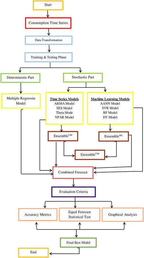
Figure 2. Pakistan electric power consumption (kWh): The developed Heterogeneous and Homogeneous Ensemble Learning Approach Layout.

3 Empirical application of the proposed ensemble technique

This study utilizes monthly averages of Pakistan’s electrical power consumption (kWh) from 1991-January to 2022-December (a total of 384 months). The statistics were acquired from the Pakistan Bureau of Statistics. To develop a dependable and effective forecasting data model, the dataset was separated into two sections: training for the model estimate and testing for an out-of-sample forecast. The training portion made use of 312 observations made between 1991-January and 2016-December. Model testing included the period from 2017-January to 2022-December, with 72 observations.

To analyze the electric power consumption time series database, this work computes the descriptive statistics (smallest, first quartile, median, arithmetic mean, mode, variance, standard deviation, third quartile, and highest values) listed in Table 2. In Table 2, the first column contains the name of each statistic; the second column in this table contains information about the original electric power consumption without any treatment; and the third column contains the natural log of the original electric power consumption time series. It is seen that after taking the natural log, the variance and standard deviation are stabilized. On the other hand, normality is also achieved, as confirmed by the mean, median, and mode, which have approximately the same values. In addition, after capturing the deterministic part (the secular long-run trend and the yearly seasonality components), the remaining series $({\mathfrak{s}}_n)$ have no evidence of seasonality, and the nonstationarity concentres. To model the stochastic component $({\mathfrak{s}}_n)$, this work used eleven different forecasting models, including four different univariate time series: the ARMA model, the SES model, the NPAR model, and the Theta model; four different univariate machine learning models: the AANN model, the SVR model, the RF model, and the DT model; and there are three novel proposed ensemble models: the time series homogeneous ensemble model, the machine learning ensemble model, and the heterogeneous ensemble model. Finally, combining the forecasting results from the deterministic and the stochastic components using Equation 9, three are eleven final forecasting models for comparison, eight are single base models, and three are the ensemble models within the proposed forecasting technique. Therefore, this study evaluates the performance of these models based on three criteria: a) accuracy metrics, b) an equal forecast statistical test, and c) a graphical assessment.Within the developed one-month-ahead electric power consumption forecasting, there are three key possibilities for comparison among the eleven forecasting models: compare the performance of eight single models, compare the performance of the proposed three ensemble models, and compare single versus the proposed ensemble models. Table 3 shows the 1-month forecast accuracy measures (MAPE, MAE, RMSE, RRSE, and CCP). Table 3 demonstrates that the ${\mathrm{E}\mathrm{n}\mathrm{s}\mathrm{e}\mathrm{m}\mathrm{b}\mathrm{l}\mathrm{e}}^{TM}$ model outperformed all other competing models, single base models, and the suggested ensemble models in terms of forecast accuracy. ${\mathrm{E}\mathrm{n}\mathrm{s}\mathrm{e}\mathrm{m}\mathrm{b}\mathrm{l}\mathrm{e}}^{TM}$ is the most effective forecasting model, with results of 5.0027, 460.4800, 614.5276, 0.2933, and 0.9560 for MAPE, MAE, RMSE, RRSE, and CCP. The ${\mathrm{E}\mathrm{n}\mathrm{s}\mathrm{e}\mathrm{m}\mathrm{b}\mathrm{l}\mathrm{e}}^{TS}$, SVR, and ARMA models achieved the second, third, and fourth-best results. However, when all single models were compared, the SVR model had the highest predicting accuracy, with the ARMA model coming in second. Among all eleven forecasting models, the ${\mathrm{E}\mathrm{n}\mathrm{s}\mathrm{e}\mathrm{m}\mathrm{b}\mathrm{l}\mathrm{e}}^{TM}$ produces more accurate forecasts than rivals’ single base models or the proposed ensemble models.

Table 2

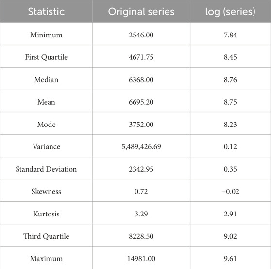
Table 2. Descriptive statistics.

Table 3

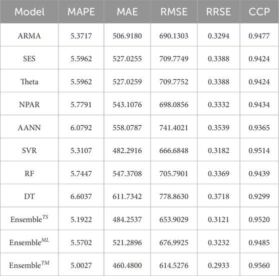
Table 3. Pakistan electric power consumption (kWh): One month ahead forecasting accuracy metrics for all eleven forecasting models within the proposed forecasting technique.

After calculating the performance metrics (MAPE, MAE, RMSE, RRSE, and CCP), we used the Diebold-Mariano (DM) test to statistically assess the superiority of models within the proposed ensemble technique (see Table 4 for p-values). Our analysis indicates a 5% significance level—the performance of eleven forecasting models, including eight base models and three proposed ensemble models. Statistical analysis (the DM test) revealed that the ${\mathrm{E}\mathrm{n}\mathrm{s}\mathrm{e}\mathrm{m}\mathrm{b}\mathrm{l}\mathrm{e}}^{TM}$ model achieved statistically superior performance across all models. Notably, the ${\mathrm{E}\mathrm{n}\mathrm{s}\mathrm{e}\mathrm{m}\mathrm{b}\mathrm{l}\mathrm{e}}^{TM}$ model also showed strong results, outperforming ten other models. Thus, these findings confirm ${\mathrm{E}\mathrm{n}\mathrm{s}\mathrm{e}\mathrm{m}\mathrm{b}\mathrm{l}\mathrm{e}}^{TM}$’s accuracy as the most reliable model for one-month-ahead electric power consumption forecasting within the scope of this study.

Table 4

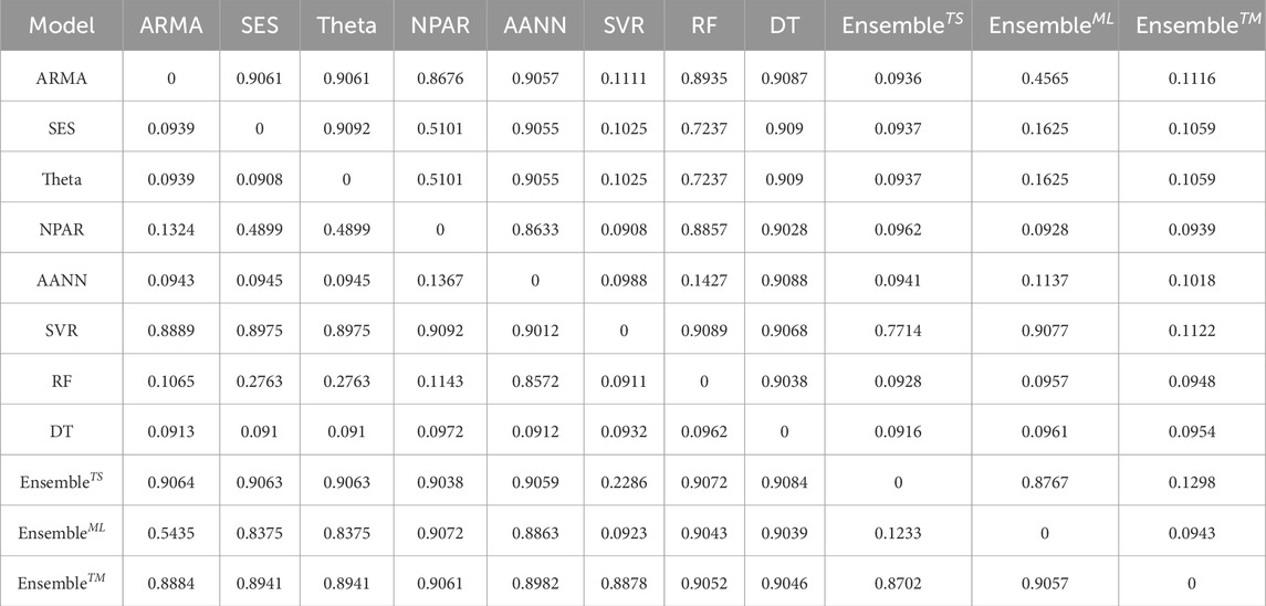
Table 4. Pakistan electric power consumption (kWh): The outcomes(p-values) of the DM test using the squared loss function for all considered forecasting models.

In addition to the above performance criteria, this comparative analysis also performed a graphical analysis to validate the current work proposed ${\mathrm{E}\mathrm{n}\mathrm{s}\mathrm{e}\mathrm{m}\mathrm{b}\mathrm{l}\mathrm{e}}^{TM}$ model’s superiority further. Figure 3 displays graphical representations of performance measurements (MAPE, MAE, RMSE, and RRSE) for all 11 models (a–d). The suggested ${\mathrm{E}\mathrm{n}\mathrm{s}\mathrm{e}\mathrm{m}\mathrm{b}\mathrm{l}\mathrm{e}}^{TM}$ model outperforms the evaluated single base and ensemble models in terms of accuracy (MAPE, MAE, RMSE, and RRSE), as shown in the figures. Additionally, the authors examined the correlogram plots (autocorrelation and partial autocorrelation) of the residuals for these three models (Figure 4). The absence of significant autocorrelation in the residuals of all models indicates that they have been sufficiently whitened, signaling satisfactory model performance. Finally, Figure 5 visually compares the actual and forecasted electric power demand for the top three models: the ${\mathrm{E}\mathrm{n}\mathrm{s}\mathrm{e}\mathrm{m}\mathrm{b}\mathrm{l}\mathrm{e}}^{TM}$ model, the ${\mathrm{E}\mathrm{n}\mathrm{s}\mathrm{e}\mathrm{m}\mathrm{b}\mathrm{l}\mathrm{e}}^{TS}$ model, and the SVR model. The ${\mathrm{E}\mathrm{n}\mathrm{s}\mathrm{e}\mathrm{m}\mathrm{b}\mathrm{l}\mathrm{e}}^{TM}$ model’s forecasts closely track the actual consumption, demonstrating its exceptional accuracy.

Figure 3

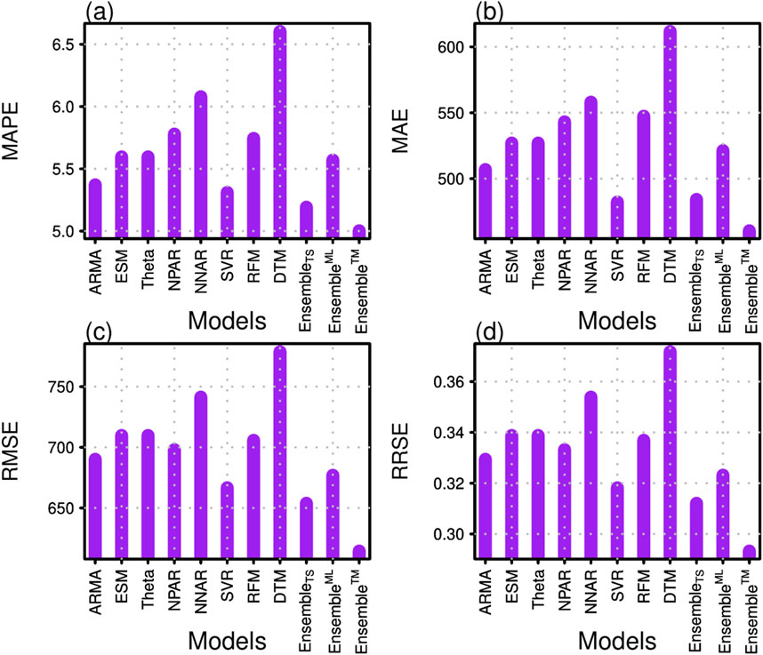
Figure 3. Accuracy metrics: (A) the MAPE, (B) the MAE, (C) RMSE, and (D) RRSE for all considered eleven forecasting models.

Figure 4

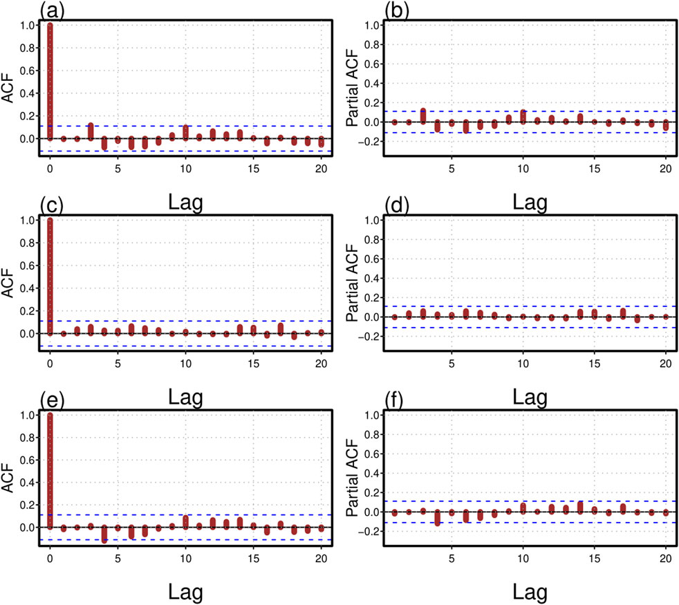
Figure 4. Autocorrelation function and partial autocorrelation plots for the three best models among all nine considered models: the ${\mathrm{E}\mathrm{n}\mathrm{s}\mathrm{e}\mathrm{m}\mathrm{b}\mathrm{l}\mathrm{e}}^{TM}$ model (A, B), the ${\mathrm{E}\mathrm{n}\mathrm{s}\mathrm{e}\mathrm{m}\mathrm{b}\mathrm{l}\mathrm{e}}^{TS}$ model (C, D), and the SVR model (E, F).

Figure 5

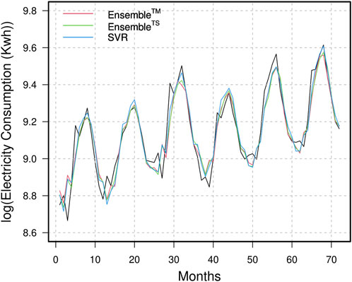
Figure 5. Comparison of Original and Forecasted Pakistan’s Electric Power consumption: the ${\mathrm{E}\mathrm{n}\mathrm{s}\mathrm{e}\mathrm{m}\mathrm{b}\mathrm{l}\mathrm{e}}^{TM}$, the ${\mathrm{E}\mathrm{n}\mathrm{s}\mathrm{e}\mathrm{m}\mathrm{b}\mathrm{l}\mathrm{e}}^{TM}$, and the SVR Models (72 Months).

Therefore, the forecasting accuracy metrics, an equal forecast statistical test, and a graphical assessment show that the proposed one-month-ahead electric power consumption forecasting technique is highly accurate and efficient. Specifically, the ${\mathrm{E}\mathrm{n}\mathrm{s}\mathrm{e}\mathrm{m}\mathrm{b}\mathrm{l}\mathrm{e}}^{TM}$ model consistently generates the most precise forecasts compared to this study’s other single and the proposed ensemble models.

4 Comparative analysis

The best model (${\mathrm{E}\mathrm{n}\mathrm{s}\mathrm{e}\mathrm{m}\mathrm{b}\mathrm{l}\mathrm{e}}^{TM}$) was selected among eleven forecasting models based on three assessment criteria: 1. accuracy average errors (MAPE, MAE, RMSE, RRSE, and CCP); 2. an equal forecast accuracy test (the DM test); and 3. graphical evaluation (line-plot, bar-plot, dot-plot, and correlogram plots). This section compares our study’s best model, ${\mathrm{E}\mathrm{n}\mathrm{s}\mathrm{e}\mathrm{m}\mathrm{b}\mathrm{l}\mathrm{e}}^{TM}$, to the best models offered in the literature as standard benchmark models. The current study discovered that this work is the best model to be highly comparable with the literature’s best proposal and the widely accepted standard benchmark techniques.

Table 5 provides a numerical comparison, while Figure 6 presents a graphical comparison of our model with other models proposed in the literature and the baseline models. Our study applied the best model proposed by Krstev et al. (2023), the neural network artificial autoregressive model (NNAR), to our dataset and calculated their average accuracy errors. The accuracy average error values reported by Krstev et al. (2023) for their best model were higher than the average error values of our best model, ${\mathrm{E}\mathrm{n}\mathrm{s}\mathrm{e}\mathrm{m}\mathrm{b}\mathrm{l}\mathrm{e}}^{TM}$. However, another study proposed a final best model (Proposed M1) Meng et al. (2011), and the authors computed their prediction accuracy average errors, which also exceeded our ${\mathrm{E}\mathrm{n}\mathrm{s}\mathrm{e}\mathrm{m}\mathrm{b}\mathrm{l}\mathrm{e}}^{TM}$ model’s average forecasting errors. Similarly, the best-proposed model (DR-SFGM) in reference Ding et al. (2022), the proposed best model (MLP) in Leite Coelho da Silva et al. (2022), and the best-proposed model (GSM) in reference Zhou et al. (2023) were comparatively worse than our best model (${\mathrm{E}\mathrm{n}\mathrm{s}\mathrm{e}\mathrm{m}\mathrm{b}\mathrm{l}\mathrm{e}}^{TM}$).

Table 5

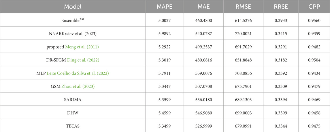
Table 5. Pakistan electric power consumption (kWh): accuracy metrics of the proposed versus the literature best and the standard baseline forecasting models.

Figure 6

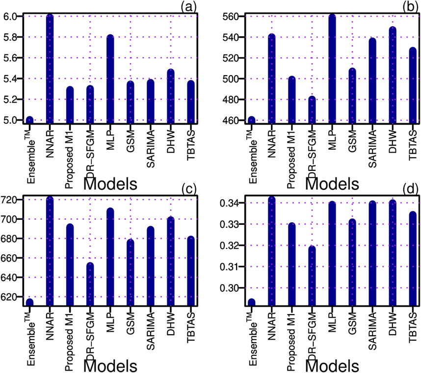
Figure 6. Accuracy performance metrics: the proposed heterogeneous ensemble model () versus the literature best models. (A) MAPE; (B) MAE; (C) RMSE, and (D) RRSE.

Additionally, we compared our best ensemble model (${\mathrm{E}\mathrm{n}\mathrm{s}\mathrm{e}\mathrm{m}\mathrm{b}\mathrm{l}\mathrm{e}}^{TM}$) with different standard benchmark models, including SARIMA, DHW, and TBATS. The comparison shows that our best model (${\mathrm{E}\mathrm{n}\mathrm{s}\mathrm{e}\mathrm{m}\mathrm{b}\mathrm{l}\mathrm{e}}^{TM}$) produces significantly more accurate and efficient outcomes than the other models. For instance, the SARIMA model produces higher mean errors and lower person correlation coefficients when compared to our heterogeneous ensemble model (${\mathrm{E}\mathrm{n}\mathrm{s}\mathrm{e}\mathrm{m}\mathrm{b}\mathrm{l}\mathrm{e}}^{TM}$). Similarly, the best outcomes are obtained by the DHW and TBTAS models, but they still show significantly worse results compared to our best forecasting model. In summary, our best heterogeneous model obtained high accuracy and efficiency compared to all competitive models, both the literature best and the baseline models, as presented in Table 5 and Figure 6.

Thus, significantly accurate and efficient monthly electric power consumption forecasting offers numerous benefits, including practical short- and medium-term strategic forecasting for lower operational and maintenance costs, improved stock and demand management, increased system reliability, and future reserves. Furthermore, monthly demand forecasting helps to reduce risks and make sound economic decisions that effect return margins, revenue, supply allocation, growth planning, inventory accounting, operating expenditures, personnel, and overall disbursement.

5 Conclusion

Understanding electricity consumption is vital for making informed decisions regarding infrastructure investment, demand planning, pricing strategies, and system reliability. Historical data analysis is essential for forecasting studies that offer insights into trends, seasonality, and peak consumption periods. This study aims to uncover the evolution of electric power consumption, which provides a foundation for accurate forecasting and assists private sector entities, regulatory bodies, and stakeholders in making informed decisions. By understanding electric power consumption evolution, authorities and private entities can take measures to ensure a stable electricity demand, supply, and system reliability. To accomplish this, the study introduces a novel approach based on ensemble learning to forecast monthly electricity consumption. The electricity consumption time series is divided into deterministic and stochastic components. The deterministic component, including a secular long-term trend and an annual seasonality, is modeled and estimated using a multiple regression model. On the other hand, the stochastic part considers the short-run random fluctuations of the consumption time series. It is modeled and forecasted by four different time-series models, four machine-learning models, and three novel proposed ensemble models: the time-series homogeneous ensemble model, the machine-learning ensemble model, and the heterogeneous ensemble model. The data used in the experiments were monthly electricity consumption data from Pakistan from 1991-January to 2022-December. The results show that the proposed ensemble models perform better than individual models, the best models reported in the literature, and are standard baseline forecasting models.

However, It was observed that the monthly pattern in our projected values shows that electricity usage is higher during the summer, with the peak demand expected in June and July. The forecast model and graph indicate a rapid increase in electricity consumption over time. This suggests that Pakistan’s government needs to enhance electricity production through various energy sources to improve the country’s economic status by meeting the electricity demand. Additionally, energy forecasting for all types of fuels and electricity by the financial sector in Pakistan can help policymakers understand future energy consumption trends and ensure a balance between energy supply and demand.

On the other hand, it should be noted that the study only focuses on Pakistan’s electric power consumption. In the future, the approach of the current research study should be extended to other countries. Additionally, the current study proposal relies on only time-series and machine-learning models and may use different models, like deep learning, in future projects within the current proposal.

Data availability statement

The data analyzed in this study is subject to the following licenses/restrictions: Data will be available on request from the corresponding author. Requests to access these datasets should be directed to hasnain@stat.qau.edu.pk.

Author contributions

HI: Conceptualization, Data curation, Formal Analysis, Funding acquisition, Investigation, Methodology, Project administration, Resources, Software, Supervision, Validation, Visualization, Writing–original draft, Writing–review and editing. JZ: Funding acquisition, Investigation, Project administration, Resources, Supervision, Writing–review and editing. Jl-G: Investigation, Project administration, Resources, Supervision, Writing–review and editing.OA: Investigation, Resources, Supervision, Writing–review and editing.

Funding

The author(s) declare that no financial support was received for the research, authorship, and/or publication of this article.

Conflict of interest

The authors declare that the research was conducted in the absence of any commercial or financial relationships that could be construed as a potential conflict of interest.

Publisher’s note

All claims expressed in this article are solely those of the authors and do not necessarily represent those of their affiliated organizations, or those of the publisher, the editors and the reviewers. Any product that may be evaluated in this article, or claim that may be made by its manufacturer, is not guaranteed or endorsed by the publisher.

References

Carbo-Bustinza, N., Iftikhar, H., Belmonte, M., Cabello-Torres, R. J., De La Cruz, A. R. H., and López-Gonzales, J. L. (2023). Short-term forecasting of ozone concentration in metropolitan lima using hybrid combinations of time series models. Appl. Sci. 13, 10514. doi:10.3390/app131810514

CrossRef Full Text | Google Scholar

Diebold, F., and Mariano, R. (1995). Comparing predictive accuracy. J. Bus. Econ. Statistics 13, 253–263. doi:10.1080/07350015.1995.10524599

CrossRef Full Text | Google Scholar

Ding, S., Tao, Z., Li, R., and Qin, X. (2022). A novel seasonal adaptive grey model with the data-restacking technique for monthly renewable energy consumption forecasting. Expert Syst. Appl. 208, 118115. doi:10.1016/j.eswa.2022.118115

CrossRef Full Text | Google Scholar

Duan, Y., Zhao, Y., and Hu, J. (2023). An initialization-free distributed algorithm for dynamic economic dispatch problems in microgrid: modeling, optimization and analysis. Sustain. Energy, Grids Netw. 34, 101004. doi:10.1016/j.segan.2023.101004

CrossRef Full Text | Google Scholar

Elsaraiti, M., Ali, G., Musbah, H., Merabet, A., and Little, T. (2021). “Time series analysis of electricity consumption forecasting using arima model,” in 2021 IEEE Green technologies conference (GreenTech) (IEEE), 259–262.

CrossRef Full Text | Google Scholar

Fan, G.-F., Wei, X., Li, Y.-T., and Hong, W.-C. (2020). Forecasting electricity consumption using a novel hybrid model. Sustain. Cities Soc. 61, 102320. doi:10.1016/j.scs.2020.102320

CrossRef Full Text | Google Scholar

Feng, J., Yao, Y., Liu, Z., and Liu, Z. (2024). Electric vehicle charging stations’ installing strategies: considering government subsidies. Appl. Energy 370, 123552. doi:10.1016/j.apenergy.2024.123552

CrossRef Full Text | Google Scholar

Gonzales, S. M., Iftikhar, H., and López-Gonzales, J. L. (2024). Analysis and forecasting of electricity prices using an improved time series ensemble approach: an application to the peruvian electricity market. AIMS Math. 9, 21952–21971. doi:10.3934/math.20241067

CrossRef Full Text | Google Scholar

Gonzalez-Briones, A., Hernandez, G., Corchado, J. M., Omatu, S., and Mohamad, M. S. (2019). “Machine learning models for electricity consumption forecasting: a review,” in 2019 2nd international conference on computer applications and information security (ICCAIS) (IEEE), 1–6.

CrossRef Full Text | Google Scholar

Hajirahimi, Z., and Khashei, M. (2023). Hybridization of hybrid structures for time series forecasting: a review. Artif. Intell. Rev. 56, 1201–1261. doi:10.1007/s10462-022-10199-0

CrossRef Full Text | Google Scholar

Hou, M., Zhao, Y., and Ge, X. (2017). Optimal scheduling of the plug-in electric vehicles aggregator energy and regulation services based on grid to vehicle. Int. Trans. Electr. Energy Syst. 27, e2364. doi:10.1002/etep.2364

CrossRef Full Text | Google Scholar

Hu, J., Zou, Y., and Soltanov, N. (2024). A multilevel optimization approach for daily scheduling of combined heat and power units with integrated electrical and thermal storage. Expert Syst. Appl. 250, 123729. doi:10.1016/j.eswa.2024.123729

CrossRef Full Text | Google Scholar

Hussain, A., Rahman, M., and Memon, J. A. (2016). Forecasting electricity consumption in Pakistan: the way forward. Energy Policy 90, 73–80. doi:10.1016/j.enpol.2015.11.028

CrossRef Full Text | Google Scholar

Iftikhar, H. (2018). Modeling and forecasting complex time series: a case of electricity demand. Pakistan: Master’s thesis, Quaid-i-Azam University Islamabad.

Google Scholar

Iftikhar, H., Bibi, N., Canas Rodrigues, P., and López-Gonzales, J. L. (2023a). Multiple novel decomposition techniques for time series forecasting: application to monthly forecasting of electricity consumption in Pakistan. Energies 16, 2579. doi:10.3390/en16062579

CrossRef Full Text | Google Scholar

Iftikhar, H., Gonzales, S. M., Zywiołek, J., and López-Gonzales, J. L. (2024a). Electricity demand forecasting using a novel time series ensemble technique. IEEE Access 12, 88963–88975. doi:10.1109/access.2024.3419551

CrossRef Full Text | Google Scholar

Iftikhar, H., Khan, M., Khan, M. S., and Khan, M. (2023b). Short-term forecasting of monkeypox cases using a novel filtering and combining technique. Diagnostics 13, 1923. doi:10.3390/diagnostics13111923

PubMed Abstract | CrossRef Full Text | Google Scholar

Iftikhar, H., Khan, M., Żywiołek, J., Khan, M., and López-Gonzales, J. L. (2024b). Modeling and forecasting carbon dioxide emission in Pakistan using a hybrid combination of regression and time series models. Heliyon 10, e33148. doi:10.1016/j.heliyon.2024.e33148

CrossRef Full Text | Google Scholar

Iftikhar, H., Khan, N., Raza, M. A., Abbas, G., Khan, M., Aoudia, M., et al. (2024c). Electricity theft detection in smart grid using machine learning. Front. Energy Res. 12, 1383090. doi:10.3389/fenrg.2024.1383090

CrossRef Full Text | Google Scholar

Iftikhar, H., Turpo-Chaparro, J. E., Canas Rodrigues, P., and López-Gonzales, J. L. (2023c). Day-ahead electricity demand forecasting using a novel decomposition combination method. Energies 16, 6675. doi:10.3390/en16186675

CrossRef Full Text | Google Scholar

Iftikhar, H., Turpo-Chaparro, J. E., Canas Rodrigues, P., and López-Gonzales, J. L. (2023d). Forecasting day-ahead electricity prices for the Italian electricity market using a new decomposition—combination technique. Energies 16, 6669. doi:10.3390/en16186669

CrossRef Full Text | Google Scholar

Iftikhar, H., Zafar, A., Turpo-Chaparro, J. E., Canas Rodrigues, P., and López-Gonzales, J. L. (2023e). Forecasting day-ahead brent crude oil prices using hybrid combinations of time series models. Mathematics 11, 3548. doi:10.3390/math11163548

CrossRef Full Text | Google Scholar

Ju, Y., Liu, W., Zhang, Z., and Zhang, R. (2022). Distributed three-phase power flow for ac/dc hybrid networked microgrids considering converter limiting constraints. IEEE Trans. Smart Grid 13, 1691–1708. doi:10.1109/tsg.2022.3140212

CrossRef Full Text | Google Scholar

Khalil, M., McGough, A. S., Pourmirza, Z., Pazhoohesh, M., and Walker, S. (2022). Machine learning, deep learning and statistical analysis for forecasting building energy consumption—a systematic review. Eng. Appl. Artif. Intell. 115, 105287. doi:10.1016/j.engappai.2022.105287

CrossRef Full Text | Google Scholar

Krstev, S., Forcan, J., and Krneta, D. (2023). An overview of forecasting methods for monthly electricity consumption. Teh. Vjesn. 30, 993–1001. doi:10.17559/TV-20220430111309

CrossRef Full Text | Google Scholar

Lei, Y., Yanrong, C., Hai, T., Ren, G., and Wenhuan, W. (2023). Dgnet: an adaptive lightweight defect detection model for new energy vehicle battery current collector. IEEE Sensors J. 23, 29815–29830. doi:10.1109/jsen.2023.3324441

CrossRef Full Text | Google Scholar

Leite Coelho da Silva, F., da Costa, K., Canas Rodrigues, P., Salas, R., and López-Gonzales, J. L. (2022). Statistical and artificial neural networks models for electricity consumption forecasting in the brazilian industrial sector. Energies 15, 588. doi:10.3390/en15020588

CrossRef Full Text | Google Scholar

Li, P., Hu, J., Qiu, L., Zhao, Y., and Ghosh, B. K. (2021). A distributed economic dispatch strategy for power–water networks. IEEE Trans. Control Netw. Syst. 9, 356–366. doi:10.1109/tcns.2021.3104103

CrossRef Full Text | Google Scholar

Meng, M., Niu, D., and Sun, W. (2011). Forecasting monthly electric energy consumption using feature extraction. Energies 4, 1495–1507. doi:10.3390/en4101495

CrossRef Full Text | Google Scholar

Meng, Q., Jin, X., Luo, F., Wang, Z., and Hussain, S. (2024). Distributionally robust scheduling for benefit allocation in regional integrated energy system with multiple stakeholders. J. Mod. Power Syst. Clean Energy. doi:10.35833/MPCE.2023.000661

CrossRef Full Text | Google Scholar

Omogoroye, O. O., Olaniyi, O. O., Adebiyi, O. O., Oladoyinbo, T. O., and Olaniyi, F. G. (2023). Electricity consumption (kw) forecast for a building of interest based on a time series nonlinear regression model. Asian J. Econ. Bus. Account. 23, 197–207. doi:10.9734/ajeba/2023/v23i211127

CrossRef Full Text | Google Scholar

Pełka, P. (2023). Analysis and forecasting of monthly electricity demand time series using pattern-based statistical methods. Energies 16, 827. doi:10.3390/en16020827

CrossRef Full Text | Google Scholar

Pham, A.-D., Ngo, N.-T., Truong, T. T. H., Huynh, N.-T., and Truong, N.-S. (2020). Predicting energy consumption in multiple buildings using machine learning for improving energy efficiency and sustainability. J. Clean. Prod. 260, 121082. doi:10.1016/j.jclepro.2020.121082

CrossRef Full Text | Google Scholar

Shah, I., Iftikhar, H., and Ali, S. (2020). Modeling and forecasting medium-term electricity consumption using component estimation technique. Forecasting 2, 163–179. doi:10.3390/forecast2020009

CrossRef Full Text | Google Scholar

Shah, I., Iftikhar, H., and Ali, S. (2022). Modeling and forecasting electricity demand and prices: a comparison of alternative approaches. J. Math. 2022. doi:10.1155/2022/3581037

CrossRef Full Text | Google Scholar

Shah, I., Iftikhar, H., Ali, S., and Wang, D. (2019). Short-term electricity demand forecasting using components estimation technique. Energies 12, 2532. doi:10.3390/en12132532

CrossRef Full Text | Google Scholar

Shirkhani, M., Tavoosi, J., Danyali, S., Sarvenoee, A. K., Abdali, A., Mohammadzadeh, A., et al. (2023). A review on microgrid decentralized energy/voltage control structures and methods. Energy Rep. 10, 368–380. doi:10.1016/j.egyr.2023.06.022

CrossRef Full Text | Google Scholar

Wang, C., Wang, Y., Wang, K., Dong, Y., Yang, Y., et al. (2017). An improved hybrid algorithm based on biogeography/complex and metropolis for many-objective optimization. Math. Problems Eng. 2017. doi:10.1155/2017/2462891

CrossRef Full Text | Google Scholar

Wang, R., Gu, Q., Lu, S., Tian, J., Yin, Z., Yin, L., et al. (2024). Fi-npi: exploring optimal control in parallel platform systems. Electronics 13, 1168. doi:10.3390/electronics13071168

CrossRef Full Text | Google Scholar

Yasmeen, F., and Sharif, M. (2014). Forecasting electricity consumption for Pakistan. Int. J. Emerg. Technol. Adv. Eng. 4, 496–503.

Google Scholar

Zhou, W., Tao, H., Chang, J., Jiang, H., and Chen, L. (2023). Forecasting Chinese electricity consumption based on grey seasonal model with new information priority. Sustainability 15, 3521. doi:10.3390/su15043521

CrossRef Full Text | Google Scholar