Dynamic balancing method of power distribution and consumption tasks based on state iterative prediction and resource peaking shifting

In the context of the new power system, the widespread access to massive distributed new energy sources has led to the power distribution and consumption tasks characterized by multiple time scales, wide random distribution, and large demand differences, resulting in unpredictable resource peaks in the tasks computing resource demand curve. In view of this situation, a method of forecasting and dynamic balancing of computing resource demand for power distribution and consumption tasks based on state iteration was proposed: firstly, the tasks computing resource demand model was established under the analysis of the attributes and parameter demand of the power distribution and consumption tasks scenario. Secondly, on the basis of the short-term effectiveness prediction of the traditional Markov model, the first-order difference of the state is used for data training to track the state fluctuation, and the historical state and the predicted state are used for state iteration, so as to avoid the convergence of long-term prediction. Finally, a dynamic balancing model is established according to the time-scale characteristics of cyclical and non-cyclical tasks, and the optimal configuration of load imbalance is achieved through the identification and adjustment of historical data and burst data. The simulation results show that the improved Markov model based on first-order difference and state iteration has the short-term accuracy of the traditional model and the long-term traceability of data fluctuations. The dynamic balancing model can combine the characteristics of historical data and burst data to effectively reduce the imbalance of resource demand, and show good ability to cope with resource imbalance deviation.

1 Introduction

The new power system is a modern power system that is efficient, flexible, and intelligent, with new energy as the main body. While developing in the future, new power systems are also facing some problems. The widespread access to new energy sources such as photovoltaics and wind power that are different from traditional energy structures has led to the power distribution and consumption tasks are characterized by multiple time scales, wide random distribution, and large demand differences (Küfeoğlu et al., 2019; Infield et al., 2020), a situation that has been led to by the widespread access to massive distributed new energy sources. Consequently, new features such as randomness and occasional demand for computing resources are presented (Xiao et al., 2023; Xiao et al., 2024). Unpredictable resource peaks in the tasks computing resource demand curve are directly led to by the characteristics of new elements, which affect the balanced relationship between resource supply and tasks demand (Cao et al., 2020; Kumar et al., 2023), making it difficult for the system to be predicted and responded to in advance (Dong et al., 2022). To reconstruct the power distribution and consumption task processing framework under the new power system, it is crucial to develop an urgent prediction solution that incorporates data mining and data reuse. Building upon this foundation, a novel solution suitable for dynamically balancing task differentiation can be explored, which fully promotes the development of distribution network automation in the new power system. (Kumar et al., 2021).

The orientation of traditional computing resource demand forecasting is towards the deconstruction and application of historical data. A cloud virtual machine resource hotspot classification mechanism is established in literature (Liu et al., 2017) to provide migration objects and targets for load prediction and dynamic scheduling. The proposal in literature (Wang et al., 2016) is to migrate high-load physical node tasks to low-load physical nodes while predicting cloud virtual machine historical data. The proposition of literature (Wang et al., 2022) is to conduct coupling dependency analysis on timing characteristics under multi-time scale tasks disassembly and fusion, thereby achieving long-term resource load prediction. Subsequent prediction based on container historical data and a large neural network model is realized in literature (Ma, 2020), which holds certain reference value for realizing dynamic prediction and resource scheduling flexibility. However, with the widespread access to massive new energy sources, traditional prediction solutions that rely solely on historical data are difficult to support, knowledge-driven ideas that take into account historical data mining and prediction data reuse have become an important driving force to improve the accuracy of demand forecasting.

The orientation of research on computing resource demand balance is towards the analysis and modeling of tasks characteristics. In terms of tasks characteristics, the feasibility of dynamically allocating processing units based on tasks characteristics is discussed in literature (Baital et al., 2020). The traditional first-come, first-served queue scheduling is changed based on tasks time characteristics in literature (Huang et al., 2018). The coupling of tasks characteristics for cluster division is considered in literature (Abbasi et al., 2021), where an affinity-based tasks scheduling algorithm is proposed. However, the identification of tasks characteristics is lacking in literature (Huang et al., 2018; Baital et al., 2020; Abbasi et al., 2021), resulting in the balanced solution not reflecting the differentiated processing process. On the topic of tasks computing resource demand modeling, tasks sequence demand is modeled based on cyclicity and similarity in literature (Alam et al., 2018). An assessment and modeling of computing resource demand for the tasks of smart distribution stations is conducted in literature (Cen et al., 2022). A deployment plan after resource assessment based on tasks characteristics and logical composition is established in literature (Zhou et al., 2022), based on (Cen et al., 2022). Although the proposal to model tasks needs is made in literature (Alam et al., 2018; Cen et al., 2022; Zhou et al., 2022), their solutions still remain at the passive assessment level and lack differentiated solution construction driven by different task perspectives.

In response to the challenges of predicting and balancing the demand curve for computing resources in power distribution and consumption tasks, a method for predicting and dynamically balancing the demand for computing resources in power distribution and consumption tasks based on state iteration is proposed in this paper. Firstly, this paper innovatively constructs a unified computing resource demand model based on the scenario attributes and parameter requirements of power distribution and consumption tasks. Secondly, this paper constructs a first-order difference model through state iteration based on the traditional Markov model. It creatively establishes a connection between historical states and predicted states, enabling continuous updates for state sequences. Finally, a dynamic balancing model is established based on the time scale characteristics of cyclical and non-cyclical tasks, and the optimal configuration of load imbalance is achieved by identifying and adjusting historical data and burst data. This paper proposes a coherent set of prediction and balancing solutions, with the goal of providing analytical tools and a foundation for equitable load balancing of computing resources in the power distribution and consumption tasks.

2 Computing resource demand model and characteristic analysis of power distribution and consumption tasks

2.1 Key issues in building computing resource demand model

Against the background of the new energy wave and digitalization wave in the power system, the demand for computing resource in the power distribution and consumption tasks has always maintained a high growth trend. However, there is often a certain lag in the configuration of terminal computing resource, which creates bottleneck constraint between computing resource demand and configuration. At the same time, due to the differences in parameter attributes of the power distribution and consumption tasks, its computing resource demand are bound to show “resource peaks” and “resource troughs” in different time periods. Therefore, it is very necessary to establish a reasonable computing resource demand model. It can not only provide mathematical model for improving the supply and demand of computing resource, but also meet the needs for flexible adjustment of resource allocation.

Drawing upon the aforementioned analysis, this chapter initiates an examination of the diverse scenario types within the power distribution and consumption tasks. Subsequently, it delves into the intricacies of the power distribution and consumption tasks’ characteristics and underscores the imperative of constructing a demand model for computing resources. Finally, from the vantage point of time, resources, and complexity, the calculation of the resource demand model for the power distribution and consumption tasks occurs across three dimensions, thereby establishing the groundwork for subsequent state prediction. The problem-solving process is depicted in Figure 1.

Figure 1

Figure 1. Flow chart of computing resource demand and characteristics analysis of power distribution and consumption tasks.

2.2 Power distribution and consumption tasks scenarios and types

The provision of a variety of services to users within the scope of the distribution network, including power supply, power quality, comprehensive energy, energy efficiency management, and market transactions, is referred to as the power distribution and consumption tasks (Chen et al., 2016). The connection of massive new energy sources such as photovoltaics, wind turbines, energy storage, and electric vehicles to the distribution network has been facilitated by the advancement of new power system transformation (Cheng, 2022). The power distribution and consumption tasks is characterized by the explosive growth of heterogeneous multi-source tasks data, resulting in large volume and variety. The typical power distribution and consumption tasks can currently be divided into two dimensions: data sensing and data applications in the entire chain utilization of power information. Data sensing, which includes online monitoring, states sensing, etc., functions to collect information from users and equipment in distribution network scenarios. Data applications, which include metering operation and maintenance, power trading, etc., can realize functions such as market transactions and rapid control.

2.3 Analysis of power distribution and consumption tasks characteristics

The power distribution and consumption tasks, which serves as an effective carrier of system informatization, automation, and intelligent upgrading and transformation, faces challenges due to its complex task characteristics, particularly in facilitating the development of distribution network interconnection. These characteristics include multiple time scales, wide random distribution, large demand differences, and parameters that are difficult to define. Owing to these characteristics, the computing resource demand curve, which is comprehensively generated by multiple types of power distribution and consumption tasks, will exhibit random and sporadic resource demand peaks. In order to proactively respond to this imbalanced state, it is urgently required to construct a multi-dimensional and fine-grained computing resource demand model from the perspective of power distribution and consumption task characteristics is urgently required.

2.4 Computing resource demand model for power distribution and consumption tasks

This section establishes a computing resource demand model based on the analysis of power distribution and consumption task characteristics. The model is expanded to include three dimensions: time, resources, and complexity: (1) Time parameters: tasks that recur at certain time intervals and tasks that do not recur at time intervals are included in power distribution and consumption tasks. The full life cycle process of these tasks encompasses arrival time, execution time, end time, and delay cycle. (2) Resource parameters: A wide range of resource demand is presented by the power distribution and consumption tasks, due to the diversification of service objects and the differentiation of processing data. (3) Complexity parameters: The degree of change in computing resource demand is referred to as the complexity of power distribution and consumption tasks, and its parameters are described by tasks sensitivity and unit scale. The task interval response time demand is referred to as its sensitivity, which is a key parameter for the dynamic and balanced deployment of tasks; The unit scale serves as a dimension for classifying task types and task needs, and is responsible for the differentiated expression of power distribution and consumption tasks.

On the basis of the definition of three types of parameter dimensions, the power distribution and consumption tasks is described in this section as a cyclical tasks model and a non-cyclical tasks model: The cyclical tasks is characterized by its fixed sampling cycle. In the power distribution scenario, to ensure the balance of “two-way power flow”, the output of distributed new energy sources needs to be quickly adjusted by the distribution network control system to deal with disturbances. These operations typically requires fixed sampling at the millisecond-level. To ensure the optimal match between electricity prices in the electricity market and real-time electricity information, rapid processing is required by the electricity market. Transaction data should be allocated reasonably to supply and demand, and this allocation usually requires fixed sampling at the second-level. In combination with parameter definition, the tasks model with a fixed sampling cycle that has been built is described as follows:

$\left\{\begin{array}{l}P{E}_{cal}^{ms}={\sum }_i{\sum }_{{\alpha }_1}P{E}_i^{cal}\left[\epsilon \left(t-{\alpha }_1{T}_i\right)-\epsilon \left(t-{\alpha }_1{T}_i-{\tau }_i\right)\right]\\ P{E}_{cal}^s={\sum }_j{\sum }_{{\alpha }_2}P{E}_j^{cal}\left[\epsilon \left(t-{\alpha }_2{T}_j\right)-\epsilon \left(t-{\alpha }_2{T}_j-{\tau }_j\right)\right]\end{array}\right.(1)$

In the formula: $P{E}_{cal}^{ms},P{E}_{cal}^s$ represent the total computing resource demand curves of millisecond-level and second-level cyclical tasks respectively. $i,j$ represent the number of millisecond-level and second-level cyclical tasks respectively. ${\alpha }_1,{\alpha }_2$ respectively represent the total number of steps in the time segment for millisecond-level cyclical tasks $i$ and second-level cyclical tasks $j$ . $P{E}_i^{cal},P{E}_j^{cal}$ respectively represent the computing resource demand of millisecond-level cyclical tasks $i$ and second-level cyclical tasks $j$ . $T_i,T_j$ respectively represent the execution cycle of millisecond-level cyclical tasks $i$ and second-level cyclical tasks $j$ . ${\tau }_i,{\tau }_j$ respectively represent the execution time of millisecond-level cyclical tasks $i$ and second-level cyclical tasks $j$.

Non-cyclical tasks are characterised by their lack of a fixed sampling cycle and their sudden nature. They often involve scenarios such as load forecasting for distribution stations and fault protection actions. The arrival time of such tasks is uncertain and the execution time is relatively long. Combined with the parameter definition, The non-cyclical tasks model constructed in this article using arrive time $t_{ar}\mathrm{,}$ execution time ${\tau }_k$ and completion time $t_{ddl}$ is described as follows:

$A{C}_k=\left(t_{ar},{\tau }_k,t_{ddl},A{C}_k^{cal}\right)(2)$

In the formula: $A{C}_k$ is used to describe the non-cyclical tasks. $A{C}_k^{cal}$ is used to describe the computing resource demand of non-cyclical tasks $k$. Based on the construction of cyclical tasks and non-cyclical tasks models, a segment division model is established for subsequent resource demand forecasting and dynamic balancing:

$\left\{\begin{array}{l}{S}_{cal}=P{E}_{cal}^{ms}+P{E}_{cal}^s+{\sum }_{k}A{C}_k^{cal}\\ S_{cal}^{ave}=\frac{{\int }_t{S}_{cal}}{t}\end{array}\right.(3)$

In the formula: $S_{cal}$ represents the multi-tasks comprehensive computing resource demand curve. $S_{cal}^{ave}$ represents the average computing resource demand. For the division of the multi-tasks comprehensive demand model into segments and the realization of the resource demand prediction, the division boundary between the resource imbalance decreasing segment and the resource imbalance increasing segment is defined by the change amount of the standard deviation of the computing resource demand and the average computing resource demand. Thus, the division judgment mechanism is thus defined:

$\left\{\begin{array}{l}{\eta }_{ba}=\sqrt{{\sum }_{\Delta t}{R}_S^{diff}{\left(S_{cal}-S_{cal}^{ave}\right)}^2}\\ \Delta {\eta }_{ba}=\sqrt{{\sum }_{\Delta t}{\left(S_{cal}-S_{cal}^{ave}\right)}^2}-\sqrt{{\sum }_{\Delta t-1}{\left(S_{cal}-S_{cal}^{ave}\right)}^2}\\ M_{cond}=\left\{\begin{array}{l}1,\Delta {\eta }_{ba}<\Delta {\eta }_{ba}^{thre}\\ 2,\Delta {\eta }_{ba}\ge \Delta {\eta }_{ba}^{thre}\end{array}\right.\end{array}\right.(4)$

In the formula: ${\eta }_{ba}$ represents the standard deviation between the computing resource demand and the average computing resource demand in $\Delta t$ . $R_S^{diff}$ represents the proportion of each value of the computing resource demand curve in $\Delta t$. $\Delta {\eta }_{ba}$ represents the change in the standard deviation of computing resource demand and average computing resource demand during $\Delta t$ . $\Delta {\eta }_{ba}^{thre}$ represents the boundary threshold that divides the resource imbalance decreasing segment and the resource imbalance increasing segment. $M_{cond}$ represents the resource imbalance state matrix. $M_{cond}=1,2$ respectively represent the decreasing resource imbalance segment and the increasing resource imbalance segment.

3 State iterative prediction model and dynamic load balancing model

3.1 Key issues in state iterative prediction model and dynamic load balancing model

Building upon the computing resource demand model for power distribution and consumption tasks, this chapter introduces an improved Markov model based on first-order differences, following the segment division framework. By incorporating first-order differences and state iteration, this approach addresses the limitations of traditional prediction models, such as insufficient posteriority and stochasticity. Furthermore, a dynamic balancing model is developed for increasing resource imbalance segment, leveraging predictive insights. This model effectively tackles the imbalance in computing resource consumption by differentially adjusting cyclical and non-cyclical tasks.

3.2 Resource demand states prediction model of power distribution and consumption tasks

To predict occasional peaks in computing resource demand, the computing resource demand curve of the power distribution and consumption tasks can be statistically constructed into a trendy and random state sequence from a statistical perspective. The Markov chain can be utilized as the applicable prediction model for the nature of this sequence. The characteristics of the traditional Markov prediction model are analysed in this chapter, and an improved Markov model based on first-order difference and sequence iterative update is proposed to ensure the accuracy and effectiveness of resource demand states prediction for the power distribution and consumption tasks.

3.2.1 Traditional Markov prediction model

The Markov prediction model is a probabilistic prediction method about the occurrence of an event. It predicts the states of the event at various times in the future based on the current states of the event. In each step of the Markov prediction model, the system can realize mutual migration between states according to the probability distribution of state transitions. This section provides an overview of the steps included in the traditional Markov prediction model. Suppose a certain system state sequence:

$X=\left\{x_1,x_2,\cdots x_n\right\}(5)$

The Markov prediction model emphasizes that the predicted state is only related to the previous state, so the transition probability between any states can be obtained based on this principle, that is, the one-step state transition matrix can be obtained:

$P^1=\left\{\begin{array}{cccc}{p}_{11}& p_{12}& \cdots & p_{1n}\\ p_{21}& p_{22}& \cdots & p_{2n}\\ ⋮& ⋮& \ddots & ⋮\\ p_{n1}& p_{n2}& \cdots & p_{nn}\end{array}\right\}(6)$

According to the current state $x_n$ of the state sequence and the one-step state transition matrix, the next state $P^1$ can be predicted:

$x_{n+1}=x_n{P}^1(7)$

Based on this, the prediction of the next stage of state can be obtained. According to the traditional Markov prediction model, the subsequent prediction is described by the k-step state transition matrix.

$x_{n+k}=x_n{P}^k=x_1{P}^{n+k}(8)$

The basic steps of the traditional Markov prediction model can be obtained from comprehensive formulas (5-8). Certain limitations are inherent in the traditional Markov model. When the curve change rate experiences sudden changes and the numerical value undergoes violent fluctuations, the complex changes that occur in the prediction process cannot be handled by a single state transition matrix. The traditional Markov model, which predicts based solely on the current state, is directly led to an inability to have aftereffects. The state value of the model will pass through the same state interval multiple times, causing the model to enter a stationary distribution and rendering it incapable of making effective predictions. In other words, the convergence of subsequent prediction data is excessively strong.

3.2.2 Improved Markov model based on first order difference and sequence iterative update

As noted in section 3.2.1, the traditional Markov model, on one hand, exhibits poor sensitivity to rate mutations and data fluctuations, and is incapable of handling complex changes that occur in the prediction process. On the other hand, its data training is based solely on historical data and lacks the reuse of prediction data, limiting the number of steps that can be accurately predicted to three to five steps. This directly results in the state prediction falling into a stationary distribution. In light of the shortcomings of the traditional Markov model, the proposal in this section is to perform first-order difference processing on the state sequence based on the accurate prediction in the previous stage of the traditional Markov model and update the prediction data to the original sequence for iteration. The first-order difference value is able to reflect not only of reflecting data fluctuations, but also of reflecting the changes in the sequence, thereby preventing the sequence prediction from developing to extremes. The scheme is depicted in Figure 2.

Figure 2

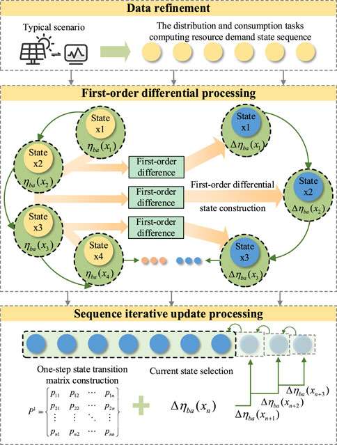
Figure 2. Improved markov prediction flowchart based on first-order differencing and iterative sequence updating.

As can be seen from Figure 2, the improved Markov model based on first-order difference and sequence iterative update includes three steps.

(1) First, the numerical sequence of power distribution and consumption tasks resource demand is constructed as:

${\eta }_{ba}\left(X\right)=\left\{{\eta }_{ba}\left(x_1\right),{\eta }_{ba}\left(x_2\right),\cdots {\eta }_{ba}\left(x_n\right)\right\}(9)$

(2) Then perform first-order difference processing on the numerical sequence of power distribution and consumption tasks resource demand, and combined with Equation 10:

$\Delta {\eta }_{ba}\left(X\right)=\left\{\Delta {\eta }_{ba}\left(x_1\right),\Delta {\eta }_{ba}\left(x_2\right),\cdots \Delta {\eta }_{ba}\left(x_{n-1}\right)\right\}(10)$

According to the resource imbalance state matrix and Equation 10, the one-step state transition matrix can be obtained by Table 1.

Table 1

Table 1. State transfer probability matrix.

In the table: $p_{11},p_{12}$ respectively represent the number of transitions from state $M_{cond}=1$ to state $M_{cond}=1,M_{cond}=2$. $p_{21},p_{22}$ respectively represent the number of transitions from state $M_{cond}=2$ to state $M_{cond}=1,M_{cond}=2$ . $P_1,P_2$ respectively represent the number of each state in the resource imbalance state matrix $M_{cond}$. In order to facilitate the calculation of subsequent state transition matrices, the initial value of the current unbalanced state $\Delta {\eta }_{ba}\left(x_n\right)$ is described by matrix $\Delta {\eta }_{ba}\left(x^{\left(n\right)}\right)$, where $\Delta {\eta }_{ba}\left(x^{\left(n\right)}\right)$ is a 1 × 2 boolean matrix, as follows:

$\left\{\begin{array}{l}\Delta {\eta }_{ba}\left(x^{\left(n\right)}\right)=\left(1,0\right),M_{cond}\left(\Delta {\eta }_{ba}\left(x_n\right)\right)=1\\ \Delta {\eta }_{ba}\left(x^{\left(n\right)}\right)=\left(0,1\right),M_{cond}\left(\Delta {\eta }_{ba}\left(x_n\right)\right)=2\end{array}\right.(11)$

In the formula: $\Delta {\eta }_{ba}\left(x^{\left(n\right)}\right)=\left(1,0\right),\Delta {\eta }_{ba}\left(x^{\left(n\right)}\right)=\left(0,1\right)$ respectively indicate that the current states is a decreasing resource imbalance segment or a increasing resource imbalance segment. According to the one-step state transition matrix $P_{cond}^1$ and the current imbalance state $\Delta {\eta }_{ba}\left(x^{\left(n\right)}\right)$ obtained in Table 1, the next stage state prediction value $\Delta {\eta }_{ba}\left(x_n\right)$ can be calculated:

$\Delta {\eta }_{ba}\left(x_{n+1}\right)=\Delta {\eta }_{ba}\left(x^{\left(n\right)}\right)P_{cond}^1(12)$

After the state transition prediction calculation, $\Delta {\eta }_{ba}\left(x_{n+1}\right)$ is a non-Boolean matrix. For subsequent calculations, $\Delta {\eta }_{ba}\left(x_{n+1}\right)$ needs to be converted into a 1 × 2 Boolean matrix:

$\left\{\begin{array}{l}\Delta {\eta }_{ba}\left(x^{\left(n+1\right)}\right)=\left(1,0\right),\mathit{max}\left(\Delta {\eta }_{ba}\left(x_{n+1}\right)\right)=\Delta {\eta }_{ba}\left(x_{n+1}\right)\left(1\right)\\ \Delta {\eta }_{ba}\left(x^{\left(n+1\right)}\right)=\left(0,1\right),\mathit{max}\left(\Delta {\eta }_{ba}\left(x_{n+1}\right)\right)=\Delta {\eta }_{ba}\left(x_{n+1}\right)\left(2\right)\end{array}\right.(13)$

According to Eq. 13, the predicted state probability can be equivalent to the segment in which the current predicted state is in resource imbalance.

(3) Finally, the predicted state is added to the original state sequence to form a new state sequence. According to the one-step state transition matrix $P_{cond}^2$ updated in Table 1 and equations (11-13), a continuous iterative prediction of the power distribution and consumption tasks resource demand state is formed:

$\left\{\begin{array}{c}\Delta {\eta }_{ba}\left(x_{n+2}\right)=\Delta {\eta }_{ba}\left(x^{\left(n+1\right)}\right)P_{cond}^2\\ ⋮\\ \Delta {\eta }_{ba}\left(x_{n+k}\right)=\Delta {\eta }_{ba}\left(x^{\left(n+k-1\right)}\right)P_{cond}^k\end{array}\right.(14)$

In the formula: $\Delta {\eta }_{ba}\left(x_{n+k}\right)$ represents the predicted state at step k. $\Delta {\eta }_{ba}\left(x^{\left(n+k-1\right)}\right)$ represents the Boolean matrix at step k-1. $P_{cond}^k$ represents the one-step state transition matrix after k updates.

Eventually, the number of steps accurately predicted by the traditional Markov front stage covers the iterative prediction sequence. In this case, accurate coverage is achieved in 3 steps. The improved Markov prediction, which is based on first-order difference and iterative sequence updating, combines the short-term accurate prediction characteristics of traditional models with the data-sensitive identification characteristics of existing models. Concurrently, the convergence of the traditional k-step state transition matrix in prediction is overcome by the addition of state iterative updates and the iteration based on a state transition matrix.

3.3 Dynamic load balancing model of power distribution and consumption tasks

Based on the prediction of computing resource demand states of power distribution and consumption tasks, reducing the peak demand for resource is an urgent issue that needs to be solved in the next step. This section considers establishing a load balancing model for the increasing resource imbalance segment. On the one hand, based on the prediction of the increasing resource imbalance segment, a dynamic balancing model for cyclical tasks based on historical data can be established; On the other hand, based on the burst characteristics of non-cyclical tasks, a non-cyclical task dynamic balancing model considering current data is established.

3.3.1 Cyclical tasks dynamic balancing model

The unbalanced increasing segment of the resource curve is attributed to the overlap of cyclical tasks, resulting in a significant gap between the resource demand curve and the average resource demand in that time cycle. In order to ensure the optimal balance of resource demand, this section combines the characteristics of cyclical tasks with fixed-interval sampling, and performs iterative updates for cyclical tasks to minimize resource imbalance based on the principle of peaking shifting. Despite the different time scales of millisecond-level cyclical tasks and second-level cyclical tasks, the adjustment ideas and principles are unified. The adjustment of second-level cyclical tasks is taken as an example for analysis in this context. The process is depicted in Figure 3.

Figure 3

Figure 3. Schematic diagram of cyclical task dynamic balancing.

As can be seen from Figure 3, this section divides the adjustment of second-level cyclical tasks into six steps:

(1) The first step is to define the first time point with the lowest resource demand of all second-level cyclical tasks in the increasing resource imbalance segment as $t_{low}^{s\_1}$.

(2) The second step is sort all second-level cyclical tasks in the increasing resource imbalance segment according to resource demand, defined as $P{E}_j^{rank}=\left\{P{E}_j^{cal\_\mathit{max}},\cdots ,P{E}_j^{cal\_\mathit{min}}\right\}$.

(3) The third step is to move the second-level cyclical task $P{E}_j^{cal\_\mathit{max}}$ to time $t_{low}^{s\_1}$ and start execution. Cyclical tasks with peaking shifting need to meet the cycle response time limit

a. When $t_{low}^{s\_1}$ is less than the cyclical response time of the task:

$P{E}_{cal}^{s\_1}={\sum }_j{\sum }_{{\alpha }_2}P{E}_j^{cal\_\mathit{max}}\left[\epsilon \left(t-t_{low}^{s\_1}-{\alpha }_2{T}_j\right)-\epsilon \left(t-t_{low}^{s\_1}-{\alpha }_2{T}_j-{\tau }_j\right)\right](15)$

In the formula: $P{E}_{cal}^{s\_1}$ represents the total resource demand of all second-level cyclical tasks after the first peaking shifting.

b. When ${\mathrm{t}}_{\text{low}}^{\mathrm{s}\_1}$ is greater than the cyclical response time of the task, the latest response time in each cycle is used as the target point for peaking shifting:

$P{E}_{cal}^{s\_1}={\sum }_j{\sum }_{{\alpha }_2}P{E}_j^{cal\_\mathit{max}}\left\{\epsilon \left[t-t_{M=2}-\left(T_j-{\tau }_j\right)-{\alpha }_2{T}_j\right]-\epsilon \left[t-t_{M=2}-\left(T_j-{\tau }_j\right)-{\alpha }_2{T}_j-{\tau }_j\right]\right.\}(16)$

In the formula: $t_{M=2}$ represents the starting point of the resource imbalance increasing segment.

(4) The fourth step involves redefining the first time point with the lowest resource demand, following the procedure outlined in step (1) and utilizing Eqs 15 and 16. Following this logic, the minimum resource demand time point sequence $t_{low}^{s\_m}$ can be obtained one after another.

(5) The fifth step involves performing the mth peaking shifting, as outlined in step (3), based on the resource demand time point sequence $t_{low}^{s\_m}$.

$P{E}_{cal}^{s\_m}={\sum }_j{\sum }_{{\alpha }_2}P{E}_j^{cal}\left[\epsilon \left(t-t_{low}^{s\_m}-{\alpha }_2{T}_j\right)-\epsilon \left(t-t_{low}^{s\_m}-{\alpha }_2{T}_j-{\tau }_j\right)\right](17)$

In the formula: $P{E}_{cal}^{s\_m}$ represents the total computing resource demand curve of second-level cyclical tasks after adjustment in the mth step.

(6) The sixth step is to define minimizing the imbalance degree as the objective optimization function and corresponding constraints:

$\mathit{min}{\eta }_{ba}^s=\sum {\omega }_t^s{\left(P{E}_{cal}^{s\_m}-P{E}_{cal}^{s\_ave}\right)}^2(18)$

s.t.

$\begin{array}{l}{C}_1:\mathit{max}\left(P{E}_{cal}^{s\_m}\right)\le C_{\text{cal}}\\ C_2:t_{low}^{s\_m}=\left\{\begin{array}{l}{t}_{low}^{s\_m},t_{low}^{s\_m}\le {\alpha }_2{T}_j\\ T_j-{\tau }_j,t_{low}^{s\_m}>{\alpha }_2{T}_j\end{array}\right.\end{array}(19)$

In the formula: ${\eta }_{ba}^s$ represents the sum of squares of the difference between the computing resource demand of all second-level cyclical tasks in the segment and the average computing resource demand. ${\omega }_t^s$ represents the time proportion of each resource value. $P{E}_{cal}^{s\_ave}$ represents the average computing resource demand of all second-level cyclical tasks in the segment. Constraint $C_1$ means that the maximum total computing resource demand of the second-level cyclical tasks after the mth step peaking shifting adjustment must not exceed the resource supply amount $C_{\text{cal}}$; Constraint $C_2$ means that peaking shifting must ensure that cyclical tasks are sampled within the response time of each cycle.

Determine whether the iteration meets the termination condition. If so, terminate it. If not, return to step (4). In the same way, the peaking shifting processing and parameter expression of millisecond-level cyclical tasks are similar to the second-level cyclical tasks.

3.3.2 Non-cyclical tasks dynamic balancing model

The previous dynamic balancing model of cyclical tasks based on historical data for state prediction has effectively reduced resource imbalance. However, due to the burst characteristics of non-cyclical tasks, the balance of the original leveling model will be broken when such tasks moves. To address this issue, this section initially distinguishes the response cycles of cyclical tasks during the non-cyclical tasks execution time. Subsequently, it performs differential leveling based on the results of this differentiation. The specific diagram is depicted in Figure 4:

Figure 4

Figure 4. Schematic diagram of non-cyclical task dynamic balancing.

As can be seen from Figure 4, the main principle of the non-cyclical tasks dynamic balancing model is to avoid cyclical tasks stagnation during its execution time: on one hand, for short-response cyclical tasks, partial avoidance can be achieved by leveraging the characteristics of their short cycle response time. on the other hand, for long-response cyclical tasks, all non-cyclical tasks can be avoided based on the characteristics of long cycle response time. According to this idea, this model uses the short response cyclical tasks back-moving time $\Delta T_d^{bm}$ and the long response cyclical tasks back-moving time $\Delta T_l^{bm}$ as decision variables to optimize the non-cyclical tasks segment to minimize the load imbalance. The specific model is as follows.

To implement this idea, the adjustable cyclical step waveform during the non-cyclical tasks time is shifted backward:

$\left\{\begin{array}{l}\Delta P{E}_{cal}^{d\left(AC\right)}=P{E}_p^{cal}\left[\epsilon \left(t-{\alpha }_3{T}_p-\Delta T_d^{bm}\right)-\epsilon \left(t-{\alpha }_3{T}_p-\Delta T_d^{bm}-{\tau }_p\right)\right]\\ \Delta P{E}_{cal}^{l\left(AC\right)}=P{E}_q^{cal}\left[\epsilon \left(t-{\alpha }_4{T}_q-\Delta T_l^{bm}\right)-\epsilon \left(t-{\alpha }_4{T}_q-\Delta T_l^{bm}-{\tau }_q\right)\right]\end{array}\right.(20)$

In the formula: $\Delta P{E}_{cal}^{d\left(AC\right)},\Delta P{E}_{cal}^{l\left(AC\right)}$ respectively represent the expressions under the final step waveform adjustment of short response cyclical tasks and long response cyclical tasks. $P{E}_p^{cal},P{E}_q^{cal}$ respectively represent the computing resource demand of short response cyclical task $p$ and long response cyclical task $q$. The meaning of parameters ${\alpha }_3,T_p,{\tau }_p$ and ${\alpha }_4,T_q,{\tau }_q$ is consistent with the previous ones, indicating the number of steps, execution cycle and execution time of short response cyclical tasks and long response cyclical tasks respectively. Reference formula (18) defines minimizing load imbalance as the objective optimization function and corresponding constraints:

$\left\{\begin{array}{l}A{C}_{cal}=A{C}_k^{cal}\left[\epsilon \left(t-t_{ar}\right)-\epsilon \left(t-t_{ar}-{\tau }_k\right)\right]\\ P{E}_{cal}^{d\_l}=\Delta P{E}_{cal}^{d\left(AC\right)}+\Delta P{E}_{cal}^{l\left(AC\right)}+A{C}_{cal}\\ +\sum P{E}_{cal}^{d\left(\neg AC\right)}+\sum P{E}_{cal}^{l\left(\neg AC\right)}\\ \mathit{min}{\eta }_{ba}^{d\_l}=\sum {\omega }_t^{d\_l}{\left(P{E}_{cal}^{d\_l}-P{E}_{cal}^{d\_l\_ave}\right)}^2\end{array}\right.(21)$

s.t.

$\begin{array}{l}{C}_1:\mathit{max}\left(P{E}_{cal}^{d\_l}\right)\le C_{\text{cal}}\\ C_2:\left\{\begin{array}{l}\Delta T_d^{bm}\le {\tau }_p\\ \Delta T_l^{bm}\le {\tau }_q\end{array}\right.\\ C_3:\left\{\begin{array}{l}\Delta T_d^{bm}+{\alpha }_3{T}_p\le t_{M=2}^{end}-{\tau }_p\\ \Delta T_l^{bm}+{\alpha }_4{T}_q\le t_{M=2}^{end}-{\tau }_q\end{array}\right.\end{array}(22)$

In the formula: $A{C}_{cal}$ represents the computing resource demand curve of non-cyclical tasks. $P{E}_{cal}^{d\_l}$ represents the total computing resource demand curve in the segment after the adjustment of the non-cyclical tasks dynamic balancing model. $P{E}_{cal}^{d\left(\neg AC\right)}$ and $P{E}_{cal}^{l\left(\neg AC\right)}$ respectively represent the computing resource demand curves of the unadjusted parts of the short response cyclical tasks and long response cyclical tasks. ${\omega }_t^{d\_l}$ represents the time proportion of each resource value after adjustment of the non-cyclical tasks dynamic balancing model. $P{E}_{cal}^{d\_l\_ave}$ represents the average computing resource demand after adjustment of the non-cyclical tasks dynamic balancing model. Constraint $C_1$ indicates that the adjusted maximum total computing resource demand must not exceed resource supply $C_{\text{cal}}$. Constraint $C_2$ means that the backward movement time does not exceed the execution time of the cyclical tasks. Constraint $C_3$ means that cyclical tasks cannot cross the current segment when avoiding non-cyclical tasks.

4 Simulation analysis

4.1 Typical scene construction

The technology for new energy sources to be widely connected to the distribution network and participate in power market regulation is becoming increasingly mature, the power distribution and consumption tasks exhibit both cyclical and non-cyclical characteristics. Therefore, this paper takes the participation of distributed photovoltaics and distributed wind power generation in response to the two-way adjustment of the power market as the research scenario. The specific tasks included in the scenario are shown in Figure 5.

Figure 5

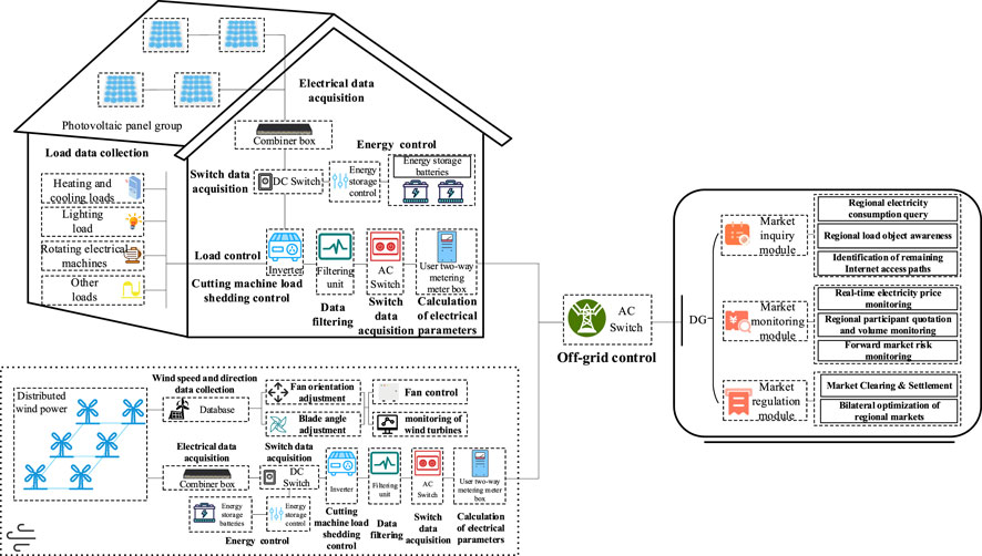
Figure 5. Typical scenarios of distributed photovoltaic and distributed wind power generation participation in two-way regulation of electricity market.

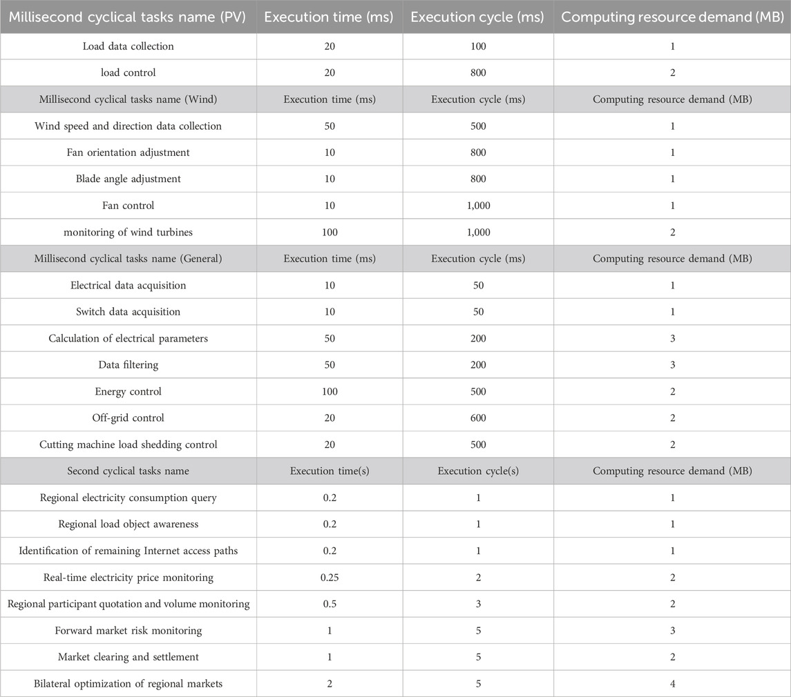
It can be seen from Figure 5 that the distributed photovoltaics and distributed wind power station area mainly undertakes millisecond-level cyclical tasks. The power market side mainly undertakes second-level cyclical tasks. This article defines computing resource capacity as 40 MB. The execution time, cycle and computing resource demand of each tasks in Figure 5 are defined, as shown in Table 2 below:

Table 2

Table 2. Cyclical task parameters.

4.2 Analysis of power distribution and consumption tasks resource demand states prediction results

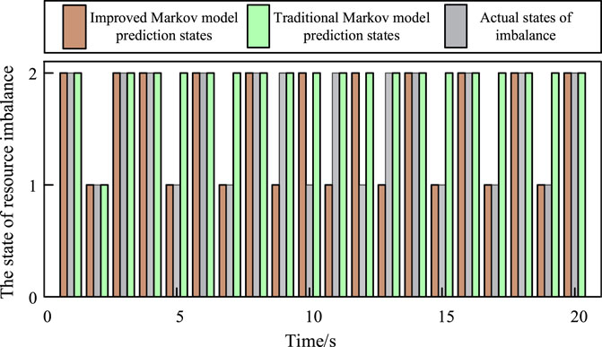
Resource states prediction requires a large amount of data for training. This section selects 0–300s as a sample of the improved Markov prediction model for first-order difference and sequence iterative update. And combine the tasks parameters in the typical scenario construction in section 4.1 to predict the resource demand states within the next 20 s. The predicted states results are shown in Figure 6.

Figure 6

Figure 6. Comparison chart of resource imbalance predictions.

It can be seen from Figure 6 that the state prediction of the improved Markov prediction model is basically consistent with the actual resource demand imbalance state. Among them: the prediction accuracy of the first 10 steps of short-term prediction is nearly 100%; the state changes of long-term prediction are also basically consistent with reality. At the same time, it can be seen from Figure 6 that the traditional Markov prediction model converges after the three-step transition, losing the effectiveness and feasibility of prediction. The simulation results prove that the improved Markov model based on first-order difference and sequence iterative update proposed in this article has the short-term accuracy of the traditional model and the long-term traceability of data fluctuations.

4.3 Analysis of results of cyclical tasks dynamic balancing model

Analyze the tasks resource demand state prediction waveform in section 4.2, and perform dynamic balancing of cyclical tasks based on historical data for the increasing resource imbalance segment in the prediction state. Here, the typical resource imbalance increasing segment 315–316s is analyzed. The waveform analysis indicators include the number of wave peaks, the highest peak difference and the stationarity: (1) The resource peak is defined as a significant protrusion in the waveform; (2) The highest peak difference is defined as the maximum resource drop at the peak before and after adjustment; (3) The stationarity is defined as the trend of resource fluctuations. The simulation of the adjusted second-level cyclical tasks, millisecond-level cyclical tasks and comprehensive cyclical tasks are as follows, as shown in Figure 7 and Table 3.

Figure 7

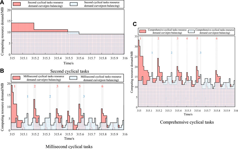
Figure 7. Comparison chart of cyclical task dynamic balancing. (A) Second cyclical tasks. (B) Millisecond cyclical tasks. (C) Comprehensive cyclical tasks.

Table 3

Table 3. Load imbalance numerical table before and after dynamic balancing (cyclical category).

It can be seen from Figure 7 that: the number of resource peaks after adjustment for millisecond-level cyclical tasks and comprehensive cyclical tasks dropped from 6 to 3; The highest peak difference of the three types of demand curves has a significant reduction effect, among which the highest peak difference of comprehensive cyclical tasks is 16MB, which proves the applicability of the dynamic balancing model; the stationarity of the three types of demand curves after adjustment is more stable than before adjustment, and the data falling points are more concentrated near the demand mean. It can be seen from Table 3 that the resource imbalance and load imbalance of second-level cyclical tasks, millisecond-level cyclical tasks and comprehensive cyclical tasks are all reduced by one order of magnitude.

Therefore, it can be proved that the cyclical tasks dynamic balancing model can fully balance the resource peaks and troughs in the forecast state, and can effectively reduce the imbalance of resource demand, thereby achieving a smooth curve.

4.4 Analysis of results of non-cyclical tasks dynamic balancing model

This section is designed to add non-cyclical tasks station load prediction in the typical resource imbalance increasing segment 315–316s in section 4.3 to verify the feasibility of the non-cyclical tasks dynamic balancing model considering current data. The parameter description of the station load forecasting task is shown in Table 4.

Table 4

Table 4. Task parameters for load forecasting in the station area.

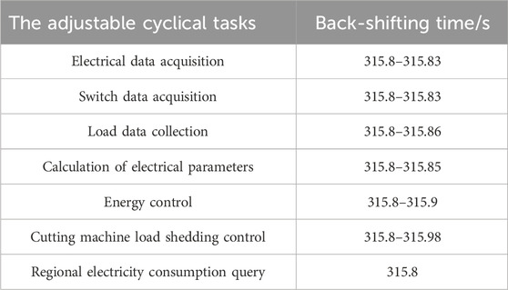
In order to achieve partial avoidance of short response cyclical tasks and complete avoidance of long response cyclical tasks, the comprehensive constraint (22) analyzes the cyclical tasks that require adjustment during the non-cyclical tasks cycle and their back-shifting time, as shown in Table 5.

Table 5

Table 5. Adjustable cyclical electric task setback timeframe during off-cycle electric tasks cycle.

According to the adjustable cyclical tasks and the corresponding back-shifting time in Table 5, a simulation analysis is conducted on the dynamic balancing model including non-cyclical tasks cycle, as shown in Figure 8 and Table 6.

Figure 8

Figure 8. Comparison chart of non-cyclical task dynamic balancing.

Table 6

Table 6. Load imbalance numerical table before and after dynamic balancing (non-cyclical category).

It can be seen from Figure 8: During the non-cyclical tasks cycle of 315.5–315.8s, the number of resource peaks before and after adjustment is significantly reduced; the highest peak difference in the segment was 5MB, which proves that leveling can completely avoid the original peak point in burst scenarios. Although the leveled curve after the segment has higher resource demand than before due to the backward shift of cyclical tasks, the data fluctuation trend ensures the data placement through the vertical increase and decrease of resources inside and outside the segment. It is more stable and meets the demand of minimizing the imbalance degree of the model. It can be seen from Table 6 that the resource demand imbalance dropped from 6.850 to 3.560 after dynamic balancing of non-cyclical tasks.

Therefore, it can be proved that the non-cyclical tasks, dynamic balancing model can make full use of current data to cope with the deviation of resource imbalance in emergency scenarios and achieve a stable demand curve.

4.5 Adaptability analysis of dynamic balancing model

4.5.1 Adaptability analysis between different segments

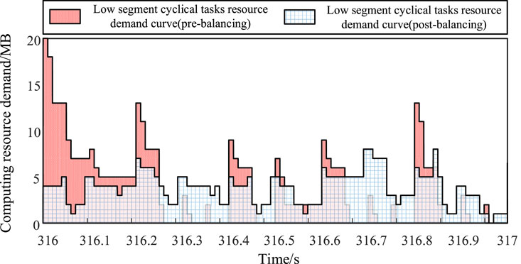
In order to further verify the applicable scope and influencing factors of the dynamic balance model, the adaptive analysis of the application of the dynamic balancing model in the resource imbalance decreasing segment is carried out. In order to facilitate the adaptability analysis between different scenarios in the following, this section only considers the role of photovoltaic scenarios, and selects the resource imbalance decreasing segment 316–317s as the research object, as shown in Figure 9 and Table 7.

Figure 9

Figure 9. Comparison chart of low segment dynamic balancing.

Table 7

Table 7. Load imbalance numerical table before and after dynamic balancing (316–317s).

It can be seen from Figure 9 that the number of peaks in this decreasing segment has dropped significantly after being adjusted by the dynamic balancing model, with the highest peak difference reaching 16MB, and the adjusted computing resource demand data points are more concentrated near the average demand line. It can be seen from Table 7 that the resource imbalance degree dropped by nearly 6 times, which is 10 times smaller than the previous increase in resource imbalance. Based on the above results, it can be seen that the dynamic balancing model is universally applicable to both the increasing and decreasing segments of resource imbalance.

On the basis of the adjusted resource imbalance decreasing segment, what factors will cause differences in dynamic balancing effects and the pros and cons brought by these differences will continue to be analyzed. Here, a simulation analysis is conducted on the change amount and change rate of computing resource demand in the two segments, as shown in Figure 10.

Figure 10

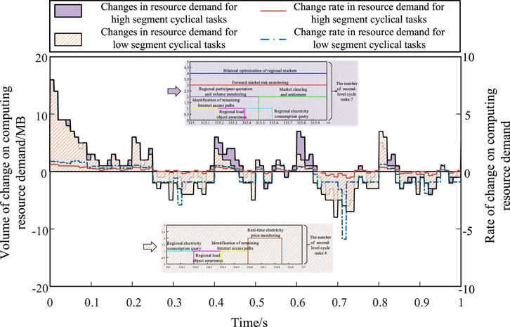
Figure 10. Comparison chart of change amount and change rate of computing resource demand in the two segments.

It can be seen from Figure 10: In terms of the change in computing resource demand, the reduction in computing resource demand in the two segments is basically synchronized. However, in terms of the increase, whether it is the horizontal time width or the vertical numerical scale, the segment where resource imbalance decreases are significantly higher than the segment where resource imbalance increases. At the same time, in terms of the change rate of computing resource demand, the fluctuation in the decreasing resource imbalance segment is more obvious than that in the increasing resource imbalance segment. Similarly, the change rate of increasing computing resources is significantly greater than that in the increasing resource imbalance segment.

Based on the above results, the composition of power distribution and consumption tasks in the two segments is further analyzed. Since millisecond-level cyclical tasks have similar distribution in the two segments, no analysis is performed here. It can be seen from the enlarged display part of the figure that the types of second-level cyclical tasks in the resource imbalance increasing segment are significantly more than those in the resource imbalance decreasing segment. The reason is that the execution cycle of second-level cyclical tasks is large, and aggregation usually occurs during its common cycle, and the segment where aggregation occurs naturally forms a increasing segment. Therefore, in the decreasing segment where there is no large accumulation of second-level cyclical tasks, the baseline value of computing resources is relatively low. Correspondingly, the possibility and rate of change of computing resources under dynamic balancing will also be relatively high.

To sum up, the execution cycle of large time-scale cyclical tasks is the main factor affecting the dynamic balancing effect. Subsequent adjustments are mainly targeted at the segments where resource imbalance increases. At the same time, the analysis of the common tasks cycle must be strengthened to achieve optimal adjustment results.

4.5.2 Adaptability analysis between different scenarios

In order to further verify the effectiveness of the dynamic balancing model in different scenarios, this section considers comparing the photovoltaic-only scenario and the wind power-only scenario, and selects the resource imbalance increasing segment 315–316s as the research object, as shown in Figure 11.

Figure 11

Figure 11. Comparison chart of change amount and change rate of computing resource demand in the two scenarios.

As can be seen from Figure 11, whether it is a separate photovoltaic scenario or a separate wind power scenario, the adaptive changes in computing resource demand reflect the universality of the dynamic balancing model in different scenarios, and also prove that the good dynamic balancing effect in the comprehensive energy scenarios in Sections 4.3 and 4.4 is not due to the role of a particular energy scenario only. Similarly, it can also be observed from Figure 11: the demand in the front stage of the wind power scenario is greatly reduced, while the demand in the back stage is increased; the overall photovoltaic scenario is relatively balanced. The reason is that the wind power scenario has a large number of proprietary tasks and a long execution cycle. Before adjustment, the demand in the front stage is large and the demand in the back stage is slightly smaller. After adjustment, there will be obvious changes in the two stages. In subsequent adjustments, consider strengthening the coordination of scenario-specific tasks features to achieve optimal adjustment results.

5 Conclusion

This paper proposes a method framework for power distribution and consumption tasks computing resource demand prediction and dynamic balancing based on state iteration. on this basis, the traditional Markov prediction scheme is improved to form an iterative prediction based on historical data and forecast data. Concurrently, an analysis is conducted on the characteristics of multi-time scale tasks based on the prediction results, leading to the formation of dynamic balancing models for different types of tasks.

(1) The improved Markov model proposed in this article based on first-order difference and sequence iterative update: on the one hand, it can reflect data fluctuations and has good tracking performance for long-sequence predictions; on the other hand, it combines the advantages of traditional models and has high accuracy for short-term predictions. This solution provides basic load state prediction solutions for industrialized intelligent terminals and is universal.

(2) The power distribution and consumption tasks load balancing model proposed in this article considers differentiated adjustments based on the characteristics of cyclical and non-cyclical tasks on the basis of state prediction: on the one hand, it fully balances the resource peaks and troughs in the predicted state, effectively reducing resource demand degree of imbalance; on the other hand, this model make full use of the cyclical tasks time response characteristics to cope with the deviation of resource imbalance in emergency scenarios, and achieve a stable demand curve.。

The following is a discussion of the limitations of the research work in this article and the directions for further research in the future: This article uses the power distribution and consumption tasks as a calculation example, but the demand prediction and dynamic balancing methods in this article are still applicable to other tasks with such characteristics. The resource demand prediction method in this article is deterministic research. In the future, the resource states in the power Internet of Things will be further complicated. How to adaptively adjust the migration boundary through uncertainty modeling of the states will be an important follow-up research direction.

Data availability statement

The original contributions presented in the study are included in the article/supplementary material, further inquiries can be directed to the corresponding author.

Author contributions

TC: Writing–review and editing. JC: Writing–review and editing. JL: Writing–review and editing. MH: Writing–original draft. XL: Writing–review and editing. ZC: Writing–review and editing. XW: Writing–review and editing.

Funding

The author(s) declare that financial support was received for the research, authorship, and/or publication of this article. This work is supported by the Science and Technology Program of China Southern Power Grid Company: Research and Application of New Energy Specialized Chip Key Technology for New Energy Monitoring and Control Demand (670000KK52220001).

Conflict of interest

Authors TC, JC, and JL were employed by China Southern Power Grid Digital Power Grid Research Institute Co. Ltd.

The remaining authors declare that the research was conducted in the absence of any commercial or financial relationships that could be construed as a potential conflict of interest.

The authors declare that this study received funding from the Science and Technology Program of China Southern Power Grid Company. The funder had the following involvement in the study: this included providing problem requirements and scenarios for the paper writing and participating in the publication of the final paper.

Publisher’s note

All claims expressed in this article are solely those of the authors and do not necessarily represent those of their affiliated organizations, or those of the publisher, the editors and the reviewers. Any product that may be evaluated in this article, or claim that may be made by its manufacturer, is not guaranteed or endorsed by the publisher.

References

Abbasi, S. I., Kamal, S., Gochoo, M., Jalal, A., and Kim, K. (2021). Affinity-based task scheduling on heterogeneous multicore systems using cbs and qbictm. Appl. Sci. 11, 5740. doi:10.3390/app11125740

CrossRef Full Text | Google Scholar

Alam, M., Rufino, J., Ferreira, J., Ahmed, H. S., Shah, N., and Chen, Y. (2018). Orchestration of microservices for IoT using docker and edge computing. IEEE Commun. Mag. 56 (9), 118–123. doi:10.1109/MCOM.2018.1701233

CrossRef Full Text | Google Scholar

Baital, K., and Chakrabarti, A. (2020). An approach: applicability of existing heterogeneous multicore real-time task scheduling in commercially available heterogeneous multicore systems. Adv. Intelligent Syst. Comput. 1042, 111–124. doi:10.1007/978-981-32-9949-8_8

CrossRef Full Text | Google Scholar

Cao, K., Liu, Y., Meng, G., and Sun, Q. (2020). An overview onEdge computing research. IEEE Access 8, 85714–85728. doi:10.1109/ACCESS.2020.2991734

CrossRef Full Text | Google Scholar

Cen, B., Hu, C., Cai, Z., Wu, Z., Zhang, Y., Liu, J., et al. (2022). A configuration method of computing resources for microservice-based edge computing apparatus in smart distribution transformer area. Int. J. Electr. Power & Energy Syst. 138, 107935. doi:10.1016/j.ijepes.2021.107935

CrossRef Full Text | Google Scholar

Chen, Y., Wu, Z., Wang, B., Ren, H., and Kong, W. (2016). Key technology of access network supporting in intelligent power distribution business. Comput. Sci. 43, 558–560.

Google Scholar

Cheng, C. (2022). Auxiliary analysis and application of Intelligent power distribution and utilization business under big data platform. Guangzhou: Guangdong University of Technology. doi:10.27029/d.cnki.ggdgu.2021.001011

CrossRef Full Text | Google Scholar

Dong, X., Chen, L., Wang, B., Shang, L., and Chen, J. (2022). Application scenario and key technology prospect of power specific integrated circuit. Proc. CSEE 42, 5017–5034. doi:10.13334/j.0258-8013.pcsee.211356

CrossRef Full Text | Google Scholar

Huang, Y.-J., Zhang, Q., Li, C.-L., Jing, M.-E., and Zeng, X.-Y. (2018). “HITSM: a heuristic algorithm for independent task scheduling in multicore,” in 2018 14th IEEE International Conference on Solid-State and Integrated Circuit Technology (ICSICT), Qingdao, China, 03 November 2018, 1–3.

CrossRef Full Text | Google Scholar

Infield, D., and Freris, L. (2020). Renewable energy in power systems. NY, USA: John Wiley & Sons.

Google Scholar

Küfeoğlu, S., Liu, G., Anaya, K., and Pollitt, M. G. (2019). Digitalisation and new business models in energy sector. Energy Policy Research Group. Cambridge, UK: University of Cambridge.

Google Scholar

Kumar, N., and Vidyarthi, D. P. (2021). A novel energy-efficient scheduling model for multi-core systems. Clust. Comput. 24 (2), 643–666. doi:10.1007/s10586-020-03143-w

CrossRef Full Text | Google Scholar

Kumar, R., and Agrawal, N. (2023). Analysis of multi-dimensional industrial IoT (IIoT) data in Edge–Fog–Cloud based architectural frameworks: a survey on current state and research challenges. J. Industrial Inf. Integration 35, 100504. doi:10.1016/j.jii.2023.100504

CrossRef Full Text | Google Scholar

Liu, W., and Li, Z. (2017). A hot-spot migration strategy for resource scheduling in cloud environment. J. Northwest. Polytech. Univ. 35, 138–142. doi:10.3969/j.issn.1000-2758.2017.01.022

CrossRef Full Text | Google Scholar

Ma, H. (2020). Research and implementation of dynamic scheduling of container cloud platform resources based on kubernetes. Nanchang: Jiangxi Normal University. doi:10.27178/d.cnki.gjxsu.2019.000436

CrossRef Full Text | Google Scholar

Wang, H., and Luo, Y. (2016). A virtual machine dynamic scheduling algorithm based on load forecast. Comput. Eng. Sci. 38, 1974–1979. doi:10.3969/j.issn.1007-130X.2016.10.004

CrossRef Full Text | Google Scholar

Wang, Y., Yu, L., Teng, F., Song, J., and Yuan, Y. (2022). Resource load prediction model based on long-short time series feature fusion. J. Comput. Appl. 42, 1508–1515. doi:10.11772/j.issn.1001-9081.2021030393

CrossRef Full Text | Google Scholar

Xiao, H., Gan, H., Yang, P., Li, L., Li, D., Hao, Q., et al. (2023). Robust submodule fault management in modular multilevel converters with nearest level modulation for uninterrupted power transmission. IEEE Trans. Power Deliv. 39, 931–946. doi:10.1109/TPWRD.2023.3343693

CrossRef Full Text | Google Scholar

Xiao, H., He, H., Zhang, L., and Liu, T. (2024). Adaptive grid-synchronization based grid-forming control for voltage source converters. IEEE Trans. Power Syst. 39 (2), 4763–4766. doi:10.1109/TPWRS.2023.3338967

CrossRef Full Text | Google Scholar

Zhou, J., Cen, B., Cai, Z., Chen, Y., Sun, Y., Xue, H., et al. (2021). Workloadmodeling for microservice-based edge computing in power internetof things. IEEE Access 9, 76205–76212. doi:10.1109/ACCESS.2021.3081705

CrossRef Full Text | Google Scholar