Advanced signal analysis for high-impedance fault detection in distribution systems: a dynamic Hilbert transform method

This paper presents a novel approach for detecting high-impedance faults (HIF) in distribution systems that uses the Hilbert transform. Our approach is based on determining the instantaneous frequency of signals and detecting deviations from a reference frequency. Our technique is very sensitive to fault fluctuations because it makes use of the Hilbert transform’s ability to capture dynamic signal properties like phase and frequency alterations. This sensitivity enables the extraction of unique features that identify fault signals, providing critical insights into fault detection and location. Notably, our method is appropriate for the analysis of non-stationary signals, which are typical in power systems where signal attributes vary fast during fault conditions. Furthermore, our method resolves deviations by comparing them to a predefined range and displaying essential features such as basic frequency, RMS (Root Mean Square), Crest Factor, Minimum and Maximum Deviations, and Maximum Current Amplitude. These values offer unique insights into the present signal’s qualities, which aids in defect detection and diagnostics, particularly in HIF settings. Our proposed technique detects high-impedance flaws by evaluating deviations from the nominal frequency, even in environments with weaker features and variable surface conditions. To improve our system’s robustness and usefulness, we recommend performing additional study on adaptive thresholding algorithms and real-time implementation choices. Future research areas could involve investigating the integration of machine learning algorithms for automatic fault categorization and localization, which would enhance the capabilities of distribution system fault detection approaches.

1 Introduction

1.1 Literature review

Ensuring the safe and reliable operation of modern power systems is of utmost importance, and one key aspect is the protection of the power system. To achieve this, electrical utilities have adopted various techniques to minimize line outages caused by short circuits. The focus has been on detecting and categorizing faults to reduce disruptions in both transmission and distribution systems ((Gogula and Edward, 2023; Ravi and Kumar, 2023)). Among the challenges encountered in this quest for reliability is the occurrence of High-Impedance Faults (HIFs) in distributor feeder networks. HIFs arise when energized conductors come into contact with high-resistance surfaces such as tree limbs, sand, and asphalt. HIFs have uneven, intermittent, and nonlinear arcing features, with fault currents ranging from 0 to 75A in grounded systems (Sedighi et al., 2005; Wang et al., 2018). If not removed promptly, HIFs can lead to severe consequences, including the destruction of conductor insulation, the occurrence of phase-to-phase faults, and risks to personal safety. Despite their significance, HIFs are often underestimated, constituting 5%–20% of total faults, although this percentage might be higher in reality. The conventional overcurrent relays commonly used for fault detection may fail to identify HIFs due to their lower current magnitude. This failure can result in cascading failures and potential fire hazards. This paper introduces a novel method for the detection of high-impedance faults in distribution systems, leveraging the capabilities of the Hilbert transform (Gogula and Edward, 2023). In a healthy power system, the fundamental frequency of the current waveform remains relatively stable. Changes in this fundamental frequency can serve as an indicator of the presence of faults or abnormal conditions. The Hilbert transform, known for its effectiveness in signal processing applications, particularly excels in capturing dynamic aspects of signals and revealing intricate details in the frequency domain. The Hilbert transform has proven to be a valuable tool in signal processing applications, particularly for its ability to capture dynamic aspects of signals and reveal intricate details in the frequency domain. In the context of distribution systems, where fault conditions demand a high level of precision in analysis, the Hilbert transform emerges as a promising technique for HIF detection. The Hilbert transform can accurately track changes in a signal’s fundamental frequency, which makes it a good tool for finding high-impedance faults (HIFs) in power systems. By analyzing the dynamic aspects of signals, the Hilbert transform can effectively identify any abnormal conditions or faults that may be present. Its ability to reveal intricate details in the frequency domain further enhances its potential as a valuable tool for precise analysis of fault conditions in distribution systems (Elkalashy et al., 2008). The utilization of high impedance fault (HIF) detection methods involving fundamental frequency, RMS (Root Mean Square), Crest Factor, and minimum and maximum deviations, along with maximum current amplitude, provides a comprehensive approach to fault analysis in distribution systems. Each of these parameters plays a crucial role in characterizing the current signal, thereby enhancing the ability to detect and diagnose HIFs. These parameters collectively provide a comprehensive approach to fault analysis, enabling a more thorough understanding of the fault behavior and aiding in its identification. Adding maximum current amplitude also makes it easier to find HIFs and makes sure that the fault detection system for distribution systems is strong. The fundamental frequency serves as a fundamental characteristic, representing the primary frequency component of the signal (Nikander and Jarventausta, 2017). Changes in the fundamental frequency can be indicative of faults, providing an initial clue to potential issues within the distribution system. This parameter is fundamental in establishing a baseline for normal operating conditions against which deviations can be assessed. By continuously monitoring the fundamental frequency, any deviations from the baseline can be quickly identified and analyzed. This allows for timely intervention and maintenance, minimizing downtime and preventing potential system failures. Additionally, the ability to detect changes in the fundamental frequency enables proactive fault detection, ensuring a reliable and efficient distribution system. RMS, or root mean square, is a measure of the overall magnitude of the current waveform. Monitoring RMS values allows for the detection of variations in signal amplitude, which is critical in identifying anomalies associated with HIFs. As high-impedance faults often result in subtle changes in current magnitude, RMS analysis provides a sensitive metric for fault detection (Doria-Garcia et al., 2020; Rahmann and Castillo, 2014). Additionally, RMS analysis can help distinguish between normal load fluctuations and abnormal conditions caused by HIFs. By comparing the RMS values to established thresholds, any significant deviations can be quickly identified and addressed, minimizing the risk of potential system failures or outages. The Crest Factor, calculated as the ratio of peak amplitude to RMS amplitude, further contributes to fault detection by highlighting the peakiness of the waveform. An increase in the Crest Factor may signify the presence of high-frequency transients or distortions associated with fault conditions. These high-frequency transients or distortions can potentially cause damage to sensitive equipment or disrupt the normal operation of the system. Therefore, monitoring and analyzing the Crest Factor can help in identifying and mitigating these issues before they lead to system failures or outages. Analyzing minimum and maximum deviations provides a dynamic perspective on frequency variations from the nominal frequency. These deviations offer insights into the transient nature of the signal, aiding in the identification of abrupt changes that may indicate the presence of faults. By comparing deviations to a predefined range, the method establishes thresholds for abnormal behavior, facilitating fault detection. This method of analyzing deviations and establishing thresholds for abnormal behavior is crucial to maintaining the reliability and stability of systems (Doria-García et al., 2021; Taheri et al., 2020). It allows for proactive measures to be taken, such as initiating maintenance or repairs, thereby preventing potential system failures or outages. Additionally, by continuously monitoring frequency variations, this approach enables the identification of emerging faults at an early stage, ensuring timely interventions to mitigate any potential risks. Maximum current amplitude, representing the highest peak value in the current waveform, is a critical parameter for detecting faults with higher magnitudes (Taheri and Hosseini, 2020; Vlahinič et al., 2021). As HIFs often result in low fault current levels, analyzing the maximum current amplitude ensures that the method remains effective in identifying faults even when fault currents are comparatively weak. By analyzing the maximum current amplitude, the approach can accurately detect faults, regardless of their magnitude (Baqui et al., 2011; Anand and Affijulla, 2020). This allows for proactive measures to be taken to prevent any further damage or disruptions in the system. Additionally, monitoring the maximum current amplitude provides valuable insights into the overall health and stability of the electrical network, allowing for more efficient maintenance and troubleshooting processes. The detection of high-impedance faults (HIFs) in power transmission lines is a critical aspect of ensuring the reliability and stability of electrical systems. While historically, research has predominantly concentrated on HIF detection in distribution systems, recent years have witnessed a shift towards addressing challenges specific to power transmission lines. This literature review provides an overview of existing methodologies for HIF detection, highlighting their strengths and limitations. Discrete wavelet transform (DWT) and root mean square (RMS) values were employed to identify and classify HIFs in distribution networks. However, the reliance on a high sampling rate for detection and the omission of method implementation during signal noise are notable drawbacks. Another approach, presented in (Nezamzadeh-Ejieh and Sadeghkhani, 2020), focuses on analyzing the time domain of current waveforms using the Kullback-Leibler divergence similarity measure. While effective in correctly identifying HIFs based on a time-based criterion, this method has limitations in terms of comprehensiveness. Time domain analysis is also explored in (Bhandia et al., 2020) for HIF detection, while (Santos et al., 2017) utilizes a transient switching method. Although the latter exhibits suitable performance, it fails to identify the faulty phase. Intelligent approaches incorporating DWT, fuzzy logic, and artificial neural networks (ANN) are discussed in (Elkalashy et al., 2008; Tonelli-Neto et al., 2017). Despite their accuracy, these methods necessitate training with diverse simulations and may exhibit sensitivity to noise. Specifically addressing HIF detection in DC microgrids, (Wang et al., 2019) proposes a scheme based on empirical mode decomposition (EMD), and (Faghihlou et al., 2020) suggests a method relying on changes in active and reactive power components. However, the latter may yield varied responses in different networks. (Sortomme et al., 2010) introduces a method utilizing current measurement at both ends of the transmission line and employing differential protection, but its dependency on telecommunication platforms poses a significant limitation. Various methods, such as correlation functions (Faridnia et al., 2012) and mathematical morphology (Gautam and Brahma, 2013; Kavi et al., 2018), are explored for fault detection. However, the computational burden on relays and the requirement for specialized equipment contribute to challenges in implementation. Traveling waves are leveraged in (Livani and Evrenosoglu, 2014) for HIF location, necessitating costly equipment for protection system deployment. Several studies, including (Ghalesefidi and Ghaffarzadeh, 2021; Faghihlou et al., 2020; Taheri and Sedighizadeh, 2020), address HIF detection as part of power swing investigations. However, these studies often lack an implemented HIF model and are limited to detecting faults with impedances below 150 Ω. In the context of this literature review, the proposed work introduces a Hilbert transform-based method for HIF detection during power swing scenarios. The methodology aims to address the shortcomings of previous studies by implementing an accurate HIF model and extending the fault detection capability to impedances above 150 Ω. The proposed approach thus contributes to advancing the state-of-the-art in HIF detection for enhanced power system reliability.

1.2 Contribution

In addition to proposing a novel method for detecting high-impedance faults (HIFs) in distribution systems, this work attempts to assess the suggested approach’s robustness, particularly in noisy situations. While the primary focus is on using the Hilbert transform and key parameters to improve fault identification, it is critical to assess the method’s efficacy under realistic settings in which noise may interfere with signal analysis.

1. Analyzing Robustness in Noisy Settings: Given the importance of noise in real-world distribution systems, we do a thorough robustness analysis to assess the effectiveness of the technique in different noise scenarios. We evaluate the method’s capacity to discriminate fault signals from background noise by injecting synthetic noise into simulated waveforms reflective of distribution system circumstances. We measure the method’s robustness against noise-induced uncertainty using statistical metrics including signal-to-noise ratio (SNR) and false positive rates.

2. Adaptive Thresholding Methods: We evaluate adaptive thresholding methods designed for dynamic signal settings in order to reduce the effect of noise on fault detection accuracy. Our approach shows enhanced sensitivity to fault signs and robustness against noise artefacts by dynamically varying detection thresholds based on signal properties and noise levels. We look into methods like adaptive filtering and wavelet-based thresholding to suppress noise interference adaptively without sacrificing fault detection capabilities.

3. Validation via Experimental Research: We verify the robustness of our approach not only via (Figures 1, 2)simulation-based assessments but also by conducting experimental research on actual distribution systems. We collect empirical evidence of our fault detection algorithm’s performance under various noise situations by deploying sensor nodes that are outfitted with it in various operational environments. We can evaluate the method’s performance in identifying HIFs in the presence of background noise and brief disturbances that arise in real-world deployment settings thanks to real-time data collecting and processing.

4. Comparison with Existing Methods: We test our approach’s performance against existing fault detection methods in noisy environments to establish a baseline for assessing its resilience. We demonstrate the benefits of our strategy in terms of robustness, sensitivity, and false alarm suppression through comparative experiments using synthetic and real-world datasets. We provide an understanding of the real-world applications of noise robustness in distribution system fault detection by methodically evaluating the advantages and disadvantages of each strategy.

Figure 1

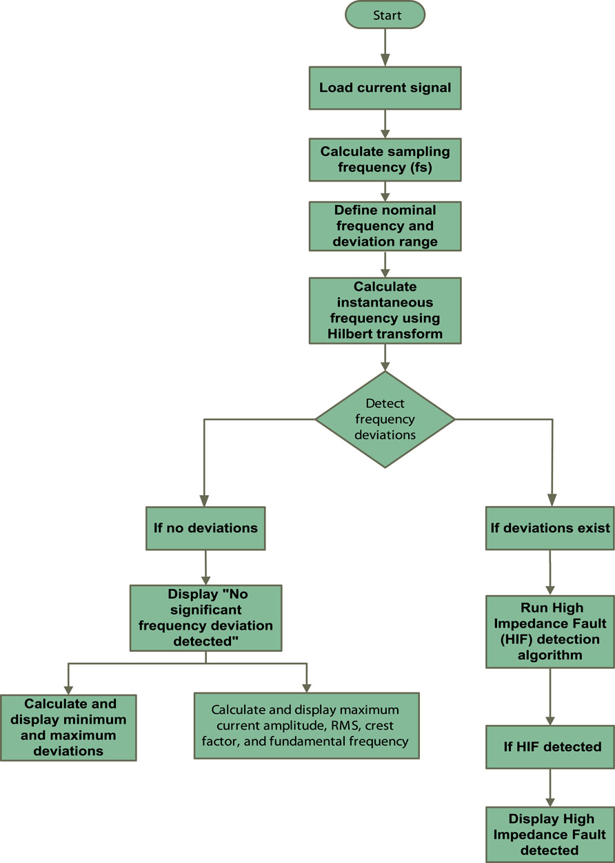
Figure 1. The algorithm proposed for detecting HIF and determining the faulty phase.

Figure 2

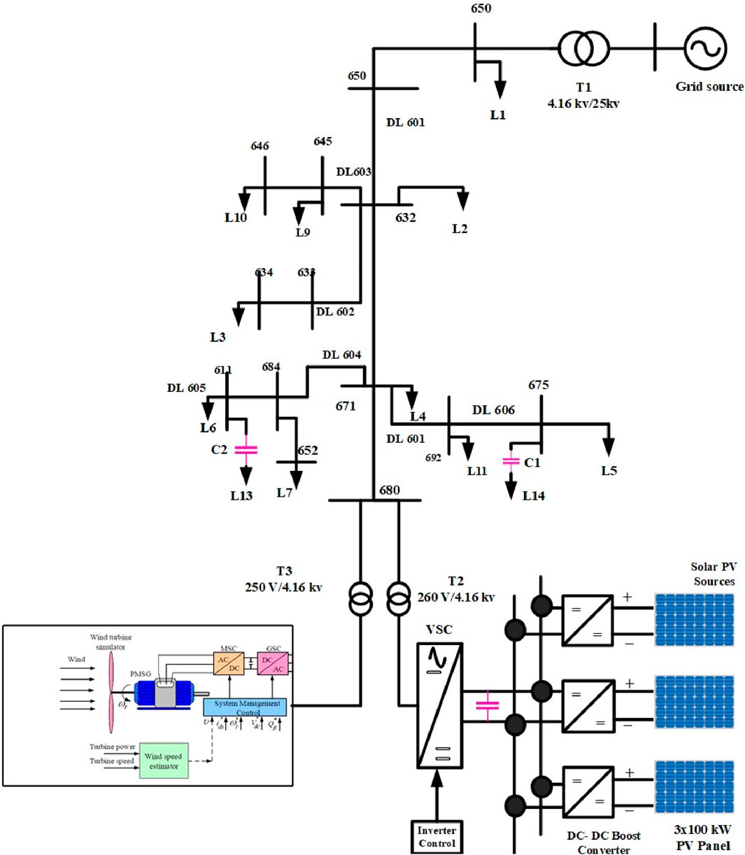
Figure 2. The single-line diagram of the network.

Our work goes beyond ensuring the development of a unique fault detection technique by adding a robustness analysis in noisy environments, guaranteeing its practical viability and reliability in real-world deployment scenarios. We show that our approach is effective in improving fault detection skills while reducing the negative effects of noise interference through thorough validation and comparative research.

2 Proposed method

The required relationships involve the calculation of the Hilbert transform, which is used to obtain the analytic representation of the voltage and current signals. By applying the Fourier transform to these analytical signals, the frequency components can be studied, and any changes that point to high-impedance faults can be found. The modified algorithm incorporates these relationships to enhance fault detection capabilities and improve overall system reliability. It talks about ways to find high-impedance faults, such as high-impedance fault detection, which involves looking at the maximum current amplitude RMS and crest factor of the current signal, comparing these values with the fundamental frequency, and using the time vector for instantaneous frequency to make fault detection more accurate.

2.1 Sampling frequency (fs)

The sampling frequency ($f_s$) is a crucial parameter in digital signal processing, and it represents the number of samples taken per unit of time. The formula to calculate the sampling frequency is given by:

$f_s=\frac{1}{\Delta t}(1)$

Where $f_s$ is the sampling frequency, Δt is the time difference between consecutive samples.

From the Nyquist-Shannon sampling theorem states that to accurately reconstruct a continuous signal from its samples, the sampling rate ($f_s$​) must be at least twice the highest frequency ($f_{\mathit{max}}$) present in the signal. This theorem is crucial in digital signal processing as it ensures that no information is lost during the sampling process. By adhering to the Nyquist-Shannon sampling theorem, we can avoid aliasing and accurately reproduce the original continuous signal from its discrete samples. Mathematically, the theorem can be expressed as:

$f_s\ge 2\cdot f_{\mathit{max}}(2)$

Where $f_s$ is the sampling frequency (samples per second or Hertz), $f_{\mathit{max}}$​ is the highest frequency component in the original continuous signal.

The sampling frequency ($f_s$) is a critical parameter in digital signal processing that characterizes the rate at which a continuous signal is discretely sampled. This fundamental quantity is determined by the reciprocal of the time difference (Δt) between consecutive samples, as expressed by Eq. 1. In practical terms, a higher sampling frequency corresponds to more samples being taken per unit of time, ensuring a more accurate representation of the original continuous signal. This process of discrete sampling is essential for converting analog signals into a digital format, facilitating their analysis and processing by digital systems. The choice of an appropriate sampling frequency is vital to avoid issues like aliasing, and adhering to the Nyquist-Shannon sampling theorem ensures that the sampling frequency is at least twice the highest frequency component present in Eq. 2.

2.2 Nominal frequency

The “nominal frequency” is a predetermined or expected frequency of a signal. It is often denoted as $f_{nominal}$. The formula for the nominal frequency is given by:

$f_{nominal}$ = Specified or Expected Frequency

This formula simply indicates that the nominal frequency is a fixed value representing the expected frequency of a signal. It serves as a reference or target frequency for comparison with the actual frequency of the signal.

In the context of the code you provided, where the nominal frequency is used for fault detection, the comparison is often done using the following equation for detecting frequency deviations:

$FrequencyDeviation=\left|instantaneousfrequency–nominalfrequency\right|(3)$

Where instantaneous Frequency is the calculated frequency of the signal at a specific time, $f_{nominal}$ ​is the nominal frequency.

Eq. 3 express as quantifies the difference between the instantaneous frequency and the nominal frequency, and deviations exceeding a specified range may indicate a fault or anomaly in the system.

The frequency deviation range is a parameter in a code that defines the allowable range within which a signal’s actual frequency can deviate from its nominal frequency without triggering a fault or alarm. It is often denoted as Δf or frequency deviation range. The code sets this range to 2 Hz. The frequency deviations are calculated by taking the absolute differences between the instantaneous and nominal frequencies at each time point. This method checks if the absolute value of the frequency deviation at any time point exceeds half of the range, indicating a potential fault.

$Thresholdlow=\frac{nominalfrequency–frequencydeviationrange}{2}(4)$

$Thresholdlow=\frac{nominalfrequency+frequencydeviationrange}{2}(5)$

These equations (4–14) calculate the lower and upper thresholds for the allowable frequency deviation range. By highlighting these thresholds on plots, you can visually assess whether the deviations fall within acceptable limits.

The frequency deviation range is set to 2 Hz. This means that any deviation from the nominal frequency by more than 2 Hz is considered a fault or anomaly.

$Frequencydeviation>\frac{Frequnecydeviationrange}{2}(6)$

The nominal frequency provides the expected frequency, the frequency deviation range sets the tolerance for acceptable deviations, and the frequency deviations are used to identify potential faults by comparing them with the specified range. This approach is commonly used in fault detection systems to assess the health and stability of signals. This combination of parameters and calculations is commonly used in fault detection systems. The frequency deviation range sets the acceptable limits for deviations, the frequency deviations quantify the actual deviations, and the fault detection threshold determines when deviations are considered significant enough to indicate a fault or anomaly in the signal.

2.3 Instantaneous frequency

The instantaneous frequency of a signal is a measure of how the frequency of the signal changes at a specific instant in time. It is a crucial concept in signal processing, and it is often calculated using the phase information of the signal.

2.3.1 Analytic signal

The analytic signal A (t) of a real-valued signal y (t) is obtained by applying the Hilbert transform. The analytic signal is a complex-valued signal that includes both the original signal and a “shifted” version of it in the imaginary part.

$A\left(t\right)=y\left(t\right)+j\cdot H\left[y\left(t\right)\right](7)$

Where j is the imaginary unit and H [y (t)] is the Hilbert transform of y (t).

The Hilbert transform is a mathematical operation used to obtain the analytic signal from a real-valued signal. The analytic signal is a complex-valued signal that contains information about both the amplitude and phase of the original signal. The Hilbert transform is particularly useful in signal processing, communications, and various other applications.

Given a real-valued signal y (t), the Hilbert transform is denoted as H[y (t)].

The Hilbert transform is typically implemented in the frequency domain by multiplying the Fourier transform of the signal by a specific kernel. The operation is defined as follows:

$H\left[y\left(t\right)\right]=\frac{1}{\pi }{\int }_{-\infty }^{\infty }\frac{y\left(\tau \right)}{t-\tau }d\tau (8)$

2.3.2 Phase of the analytic signal

The instantaneous frequency is related to the phase of the analytic signal. The phase ϕ (t) is obtained from the complex analytic signal.

$\varphi \left(t\right)=\mathit{arctan}\left(\frac{Im\left[A\left(t\right)\right]}{Re\left[A\left(t\right)\right]}\right)(9)$

Where $\text{Im\hspace{0.17em}}\left[A\left(t\right)\right]$ part of the imaginary and is the real part of the analytic signal.

2.3.3 Instantaneous frequency

The instantaneous frequency f (t) is then calculated as the rate of change of the phase with respect to time.

$f\left(t\right)=\frac{1}{2\pi }\frac{d\varphi \left(t\right)}{dt}(10)$

Here, $\frac{d\varphi \left(t\right)}{dt}$ represents the derivative of the phase with respect to time.

The entire process involves transforming the original signal into an analytic signal, extracting the phase information, and then deriving the instantaneous frequency from the phase. This allows us to understand how the frequency of the signal changes at each point in time, providing valuable insights into time-varying behavior. These formulas are fundamental in signal processing and are commonly used to analyze signals in various applications.

2.3.4 Maximum current amplitude

The Maximum Current Amplitude ($I_{\mathit{max}}$) is a crucial parameter in power system analysis, protection, and equipment design, representing the highest instantaneous value of the current waveform during a specific time period. Mathematically, it is calculated as the maximum absolute value of the current ($I\left(t\right)$) at any given time:

$I_{\mathit{max}}=\max \left(\left|I\left(t\right)\right|\right)(11)$

Here, $I\left(t\right)$ denotes the instantaneous current, and max (($\left|I\left(t\right)\right|$) identifies the peak absolute value of the current.

The maximum current amplitude ($I_{\mathit{max}}$) is a crucial parameter in power system analysis, protection, and equipment design. It represents the highest instantaneous value of the current waveform during a specific time period. Factors contributing to maximum current amplitude include tree limbs near power lines, which can lead to faults, corona discharge, and soil resistance. The moisture content in sand significantly impacts soil resistivity and impedance, affecting grounding electrode performance. Sand is also used as bedding material for underground cables, influencing their thermal characteristics, impedance, and heat dissipation. These factors can lead to power losses and radio frequency interference.

2.3.5 Root mean square (RMS) current

The RMS current (Irms​) is a measure of the effective or heating value of a current waveform. It quantifies the equivalent direct current that would produce the same heating effect as the alternating current. The formula for calculating the RMS current is:

$I_{rms}=\sqrt{\frac{1}{T}{\int }_0^T{\left[I\left(t\right)\right]}^{2}dt}(12)$

Where I (t) represent the instantaneous current at any given time, T is the period of the waveform.

The RMS current is calculated by taking the square root of the average of the squared instantaneous values over one complete period of the waveform. Understanding the RMS value is important because it provides a single value that characterizes the magnitude of the current waveform, making it easier to compare and analyze. It is commonly used in various applications, including determining equipment ratings, evaluating the thermal impact on components, and setting protection relay thresholds.

2.3.6 Crest factor

The Crest Factor (CF) is a measure of the shape of a waveform, indicating how “peaky” or “flat” the waveform is. It is the ratio of the peak value of the waveform to its RMS value. The formula for calculating the Crest Factor is:

$\text{CF}=\frac{\text{Peak}\text{value}}{\text{RMS}\text{value}}(13)$

Alternatively, the Crest Factor can be calculated using the peak-to-peak value (Ipp) and the RMS value:

$CF=\frac{I_{PP}}{2\cdot I_{rms}}(14)$

Where Peak Value is the maximum absolute value of the waveform, RMS Value is the Root Mean Square value of the waveform, Ipp ​ is the peak-to-peak value of the waveform.

A higher Crest Factor indicates a peakier waveform, while a lower Crest Factor suggests a flatter waveform. Crest Factor is important in power system analysis, especially in applications where the peak amplitude of the waveform is critical, such as in sizing components to withstand transient conditions. It is also used in audio and signal processing to characterize the dynamic range of a signal.

2.3.7 Minimum and maximum frequency deviations

Frequency deviations refer to the difference between the actual instantaneous frequency of a signal and its nominal or expected frequency. These deviations can be calculated at each time point, and the minimum and maximum deviations are important indicators in assessing the stability and health of a system.

Frequency Deviation at Time t: The frequency deviation at any given time t is calculated as the absolute difference between the instantaneous frequency (f (t)) and the nominal frequency (fnominal):

$Frequencydeviationattimet=\left|f\left(t\right)-f_{nominal}\right|(15)$

Minimum Frequency Deviation (fmin): The minimum frequency deviation is calculated as the smallest absolute frequency difference observed over a specific time period:

$f_{\mathit{min}}=\min \left(\left|f\left(t\right)-f_{nominal}\right|\right)(16)$

Where f (t) is the instantaneous frequency at any given time, and fnominal ​is the nominal frequency.

Maximum Frequency Deviation (fmax): The maximum frequency deviation is calculated as the largest absolute frequency difference observed over a specific time period:

$f_{\mathit{max}}=\max \left(\left|f\left(t\right)-f_{nominal}\right|\right)(17)$

Where f (t) is the instantaneous frequency at any given time, and fnominal is the nominal frequency.

These Eqs 15–17 represent the minimum and maximum deviations from the nominal frequency at different time points, providing a quantitative measure of the frequency variations in the system. In the context of the provided code, these calculations help identify the range of frequency deviations and assess the severity of deviations from the expected or nominal frequency.

2.3.8 Fundamental frequency

The Fundamental Frequency ($f_0$) is the lowest frequency component of a periodic waveform. It is the frequency at which the waveform oscillates with the greatest amplitude and repeats most frequently. In the context of a current signal, the fundamental frequency often corresponds to the power system frequency. Eq. 18 for calculating the Fundamental Frequency depends on the signal processing technique used. From Figure 3 the sinusoidal waveform, the fundamental frequency is simply the frequency of the sinusoid. In the context of analyzing a complex waveform, the Fundamental Frequency can be determined from the spectrum analysis, such as by identifying the peak frequency in the frequency domain.

Figure 3

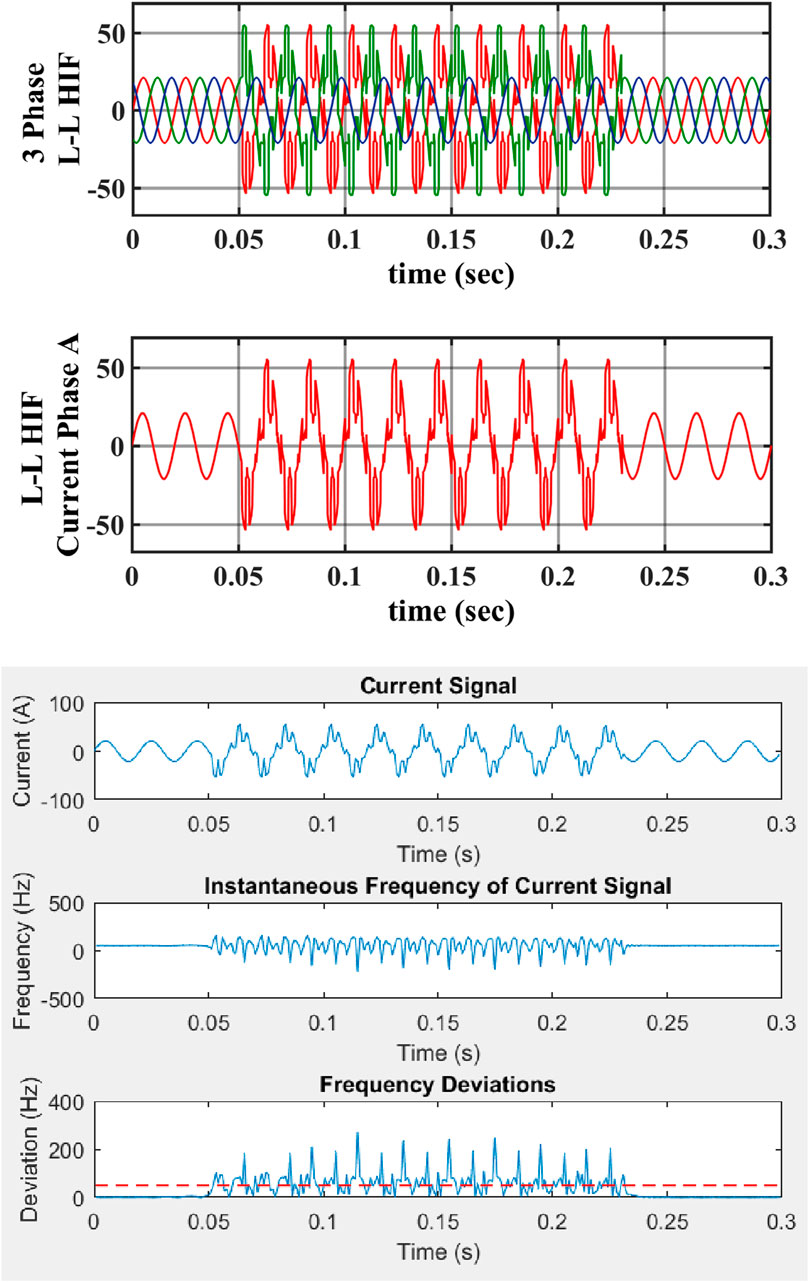
Figure 3. HIF faults detection by frequency at resistance 50 Ω.

For a sinusoidal waveform with frequency $f_0$​, the formula is expressed as:

$f_0=\frac{1}{T}(18)$

Where $f_0$ the Fundamental Frequency, T is the period of the waveform. In power systems, the Fundamental Frequency is often set by the design of the power grid. In power system many regions, the power system operates at a frequency of 50 or 60 Hz. Deviations from this frequency can indicate issues in the power system. With these Fundamental Frequency is essential for various applications, including power quality analysis, harmonic analysis, and fault detection in electrical systems.

2.4 Hybrid IEEE 13 bus distribution system operation

The proposed system combines solar, wind, battery, and fuel cell power technologies to create a hybrid renewable energy storage solution. This system ensures continuous energy generation, while battery and fuel cell technologies offer efficient storage and backup options. This approach maximizes renewable resource utilization and reduces reliance on traditional fossil fuels, contributing to a greener and more resilient energy infrastructure. The system is connected to the IEEE 13 bus distribution system for seamless integration with existing power infrastructure. This connection allows the system to feed any extra energy it produces back into the grid, promoting renewable energy use and potentially reducing consumer electricity costs. Additionally, being connected to the grid provides a reliable backup option in case of fluctuations or shortages in renewable energy generation. Advanced Hilbert transform fault detection algorithms and technologies can be implemented to quickly identify and isolate faults, minimizing downtime and ensuring uninterrupted power supply to consumers.

3 Results and discussion

The Hilbert transform is a mathematical tool that can be used to analyze high-impedance faults in hybrid renewable energy storage systems. It can be used in MATLAB simulations to accurately detect and diagnose these faults, ensuring smooth system operation and preventing potential damage. The Hilbert transform can help detect frequency analysis and abnormalities in the system’s frequency response, providing valuable insights into the magnitude and phase of the system’s frequency components. This Table 1 analysis can help determine the root cause of high impedance faults, enabling timely corrective actions, minimizing downtime, and maximizing system performance. The MATLAB simulation can be used for frequency analysis and identifying abnormalities in the system’s frequency response, enabling engineers to identify fault characteristics and take corrective action, ensuring minimal downtime and optimal system performance.

Table 1

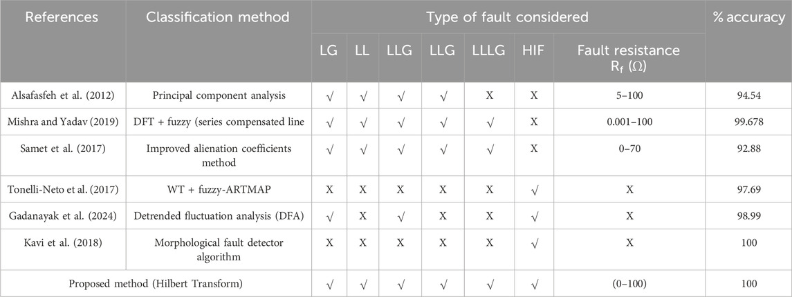
Table 1. Comparative analysis of Electrical-based HIF detection techniques.

3.1 HIF fault detection in IEEE 13 bus distribution system

3.1.1 L-G fault detected by Hilbert transform

Power systems are susceptible to disturbances and anomalies, such as voltage fluctuations, frequency variations, and sudden load changes, which can lead to equipment damage, power outages, and system-wide failures if not managed properly. High-impedance faults (HIFs) are particularly challenging due to their limited fault current, which can be close to the minimum current the power system can handle. This can reduce power system stability and reliability. HIFs can also cause voltage dips and flickers, disrupting the normal operation of electrical equipment. Regular protection schemes may not accurately detect HIFs, leading to delayed isolation. Specialized protection devices and algorithms are needed to accurately detect and mitigate HIFs, ensuring system stability and reliability. Continuous monitoring and analysis of power system parameters are essential for identifying potential HIF events and implementing preventive measures. The Hilbert transform is a commonly used fault detection technique in power systems, allowing operators to quickly locate and address faulty sections, preventing widespread disruptions, and ensuring the smooth functioning of the electrical grid. This Hilbert transform can detect the exact frequency and magnitude of power system signals, allowing operators to identify abnormalities and potential faults. By accurately analyzing the frequency and magnitude of current, the Hilbert transform helps in maintaining the stability and reliability of the power system by enabling timely interventions and preventive measures. To test how well the suggested method works with different types of HIFs, a single-phase HIF is first selected for evaluation. The fault is applied to phase A, with different resistance ranges from R = 25 Ω to R = 1,200 Ω. The selected single-phase HIF is connected to a power source, and the fault parameters are adjusted accordingly. The evaluation process includes monitoring the voltage and current responses of phase A to analyze the effectiveness of the suggested method. The evaluation process also involves measuring the fault current magnitude and duration to further assess the performance of the selected single-phase HIF. Additionally, as shown in Figure 4, the THD value of 11.06% indicates a moderate level of distortion, which suggests that further improvements may be needed to optimize the suggested method’s effectiveness. The current amplitude and frequency of the fault are recorded and compared to the normal operating conditions as shown in Figure 5. Analysis of the current waveforms identifies any anomalies or deviations brought on by the fault. In this high-impedance fault detection process, set the constant frequency deviation at 50 Hz. When the fault occurs, the frequency will increase above the constant frequency deviation. This method allows for the detection of high impedance faults by monitoring changes in frequency deviation above the set constant frequency deviation. By analyzing the fundamental frequency range, RMS range, crest factor, and maximum current amplitude range, potential faults can be identified and addressed promptly. As shown in Figure 6, in normal conditions, the fundamental frequency range is 261.69 Hz, the RMS (root mean square) range is 14.8764 A, the crest factor is 1.4147, the minimum and maximum deviations are 0.00 Hz and 1.06 Hz, and the maximum current amplitude range is 21.0462 A. Also, as shown in Figure 7, the high impedance fault is in phase A at resistance 25 Ω. This condition will also be measured in terms of fundamental frequency, RMS (root mean square), crest factor, minimum and maximum deviations, and maximum current amplitude. The high-impedance faults are at resistance 25 Ω. The fundamental frequency range is 261.66 Hz, the RMS (root mean square) range is 21.4294 A, the crest factor is 1.9844, the minimum and maximum deviations are 0.02 and 214.41 Hz, and the maximum current amplitude range is 42.5254 A.

Figure 4

Figure 4. MATLAB/SIMULINK model of high impedance fault.

Figure 5

Figure 5. THD value of HIF fault current Phase A.

Figure 6

Figure 6. HIF faults detection by frequency at normal condition.

Figure 7

Figure 7. HIF faults detection by frequency at resistance 25Ω.

3.1.2 L-L fault detected by Hilbert transform

High impedance faults occur when foreign objects, such as tree limbs, sand, or soil, come into contact with power lines, disrupting the flow of electricity. Weather conditions, such as strong winds or heavy rain, can also increase the likelihood of such faults. In such situations, a line-to-line high impedance fault can occur, causing changes in current amplitude and frequency. The Hilbert transformer can be used to analyze high-impedance faults, identifying high-frequency components in the power system. By applying the Hilbert transform to current waveforms, engineers can detect and locate faults, allowing for timely repairs and maintenance to prevent further disruptions in electricity flow. Accurate frequency deviation detection, as shown in Figure 7, is crucial in identifying faults and abnormalities in the power system, enabling prompt corrective action. The Hilbert transform can also help analyze power quality issues and improve overall system performance by providing valuable insights into voltage and current waveforms. It can detect and calculate the fundamental frequency range, RMS (root mean square), crest factor, minimum and maximum deviations, and maximum current amplitude range, helping engineers identify fault characteristics and determine corrective measures. By accurately measuring these parameters, the Hilbert transform assists in identifying the root causes of power quality issues and enables engineers to implement targeted solutions. Additionally, the analysis that the Hilbert transform provides can help predict potential system failures and reduce expensive downtime by enabling proactive maintenance and repairs. The Hilbert transform can detect a line-to-line high-impedance fault at 25 Ω resistance and can be used to calculate the fundamental frequency range of 261.64 Hz. The RMS (root mean square) is 24.5017. The crest factor is 2.2624, and the minimum and maximum deviations are 0.02 Hz and 271.69 Hz. The maximum current amplitude range is 55.4328 A.

The Hilbert transform is a mathematical tool used to analyze the instantaneous amplitude and phase of a signal. By applying the Hilbert transform to the current waveforms, it is possible to identify high-impedance faults with varying resistance values, as shown in Table 2. This is particularly useful in power systems, where high-impedance faults can be challenging to detect using traditional methods. The Hilbert transform allows for a more accurate and efficient fault identification process, improving the overall reliability and stability of the system.

Table 2

Table 2. HIF detection with different resistance values.

4 Conclusion

In this study, we introduced a novel approach for high-impedance fault detection in distribution systems, leveraging the Dynamic Hilbert Transform method. Through a comprehensive analysis of signal characteristics, our proposed method demonstrates promising results in accurately identifying high-impedance faults, thereby addressing a critical challenge in power distribution systems. Our research highlighted the limitations of existing detection methods, underscoring the need for advanced signal analysis techniques. The Dynamic Hilbert Transform method proved to be an effective tool in extracting relevant information from complex signals, enabling robust fault detection even in scenarios with varying system dynamics. The experimental results presented in this paper showcased the superior performance of our proposed method compared to traditional techniques. The ability to detect high-impedance faults promptly is crucial for preventing potential equipment damage, minimizing downtime, and enhancing overall system reliability. Furthermore, the adaptability of the Dynamic Hilbert Transform to dynamic system conditions positions it as a versatile solution for fault detection in real-world distribution networks. The incorporation of this method into existing protective relaying systems holds the potential to significantly improve fault detection capabilities and contribute to the overall resilience of power distribution infrastructures. As we look ahead, ongoing research in this field should explore the integration of our proposed method into practical applications and address potential challenges in real-world deployment. This research contributes to the ongoing efforts to enhance the reliability and efficiency of power distribution networks, ultimately fostering a more resilient and sustainable energy future.

Data availability statement

The original contributions presented in the study are included in the article/Supplementary Material, further inquiries can be directed to the corresponding author.

Author contributions

VG: Writing–original draft, Writing–review and editing. BE: Writing–review and editing.

Funding

The author(s) declare that no financial support was received for the research, authorship, and/or publication of this article.

Conflict of interest

The authors declare that the research was conducted in the absence of any commercial or financial relationships that could be construed as a potential conflict of interest.

Publisher’s note

All claims expressed in this article are solely those of the authors and do not necessarily represent those of their affiliated organizations, or those of the publisher, the editors and the reviewers. Any product that may be evaluated in this article, or claim that may be made by its manufacturer, is not guaranteed or endorsed by the publisher.

References

Alsafasfeh, Q., Abdel-Qader, I., and Harb, A. (2012). Fault classification and localization in power systems using fault signatures and principal components analysis. Energy Power Eng. 4 (6), 506–522. doi:10.4236/epe.2012.46064

CrossRef Full Text | Google Scholar

Anand, A., and Affijulla, S. (2020). Hilbert-Huang transform based fault identification and classification technique for AC power transmission line protection. Int. Trans. Electr. Energy Syst. 30 (10). doi:10.1002/2050-7038.12558

CrossRef Full Text | Google Scholar

Baqui, I., Zamora, I., Mazón, J., and Buigues, G. (2011). High impedance fault detection methodology using wavelet transform and artificial neural networks. Electr. Power Syst. Res. 81 (7), 1325–1333. doi:10.1016/j.epsr.2011.01.022

CrossRef Full Text | Google Scholar

Bhandia, R., Chavez, J. D. J., Cvetkovic, M., and Palensky, P. (2020). High impedance fault detection using advanced distortion detection technique. IEEE Trans. Power Deliv. 35 (6), 1. doi:10.1109/tpwrd.2020.2973829

CrossRef Full Text | Google Scholar

Doria-Garcia, J., Orozco-Henao, C., Iurinic, L. U., and Pulgarín-Rivera, J. D. (2020). High impedance fault location: generalized extension for ground faults. Int. J. Electr. Power Energy Syst. 114, 105387. doi:10.1016/j.ijepes.2019.105387

CrossRef Full Text | Google Scholar

Doria-García, J., Orozco-Henao, C., Leborgne, R., Montoya, O. D., and Gil-González, W. (2021). High impedance fault modeling and location for transmission line. Electr. Power Syst. Res., 196. doi:10.1016/j.epsr.2021.107202

CrossRef Full Text | Google Scholar

Elkalashy, N. I., Lehtonen, M., Darwish, H. A., Taalab, A. M. I., and Izzularab, M. A. (2008). DWT-based detection and transient power direction-based location of high-impedance faults due to leaning trees in unearthed MV networks. IEEE Trans. Power Deliv. 23 (1), 94–101. doi:10.1109/tpwrd.2007.911168

CrossRef Full Text | Google Scholar

Faghihlou, M., Taheri, B., and Salehimehr, S. (2020) “High impedance fault detection in dc microgrid using real and imaginary components of power,” in 2020 28th Iranian conference on electrical engineering, ICEE 2020.

CrossRef Full Text | Google Scholar

Faridnia, N., Samet, H., and Doostani Dezfuli, B. (2012). A new approach to high impedance fault detection based on correlation functions. IFIP Adv. Inf. Commun. Technol. 381 (PART 1), AICT.

CrossRef Full Text | Google Scholar

Gadanayak, D. A., Mishra, M., and Bansal, R. C. (2024). High impedance fault detection in distribution networks using randomness of zero-sequence current signal: a detrended fluctuation analysis approach. Appl. Energy 368, 123452. doi:10.1016/j.apenergy.2024.123452

CrossRef Full Text | Google Scholar

Gautam, S., and Brahma, S. M. (2013). Detection of high impedance fault in power distribution systems using mathematical morphology. IEEE Trans. Power Syst. 28 (2), 1226–1234. doi:10.1109/tpwrs.2012.2215630

CrossRef Full Text | Google Scholar

Ghalesefidi, M. M., and Ghaffarzadeh, N. (2021). A new phaselet-based method for detecting the power swing in order to prevent the malfunction of distance relays in transmission lines. Energy Syst. 12 (2), 491–515. doi:10.1007/s12667-019-00366-8

CrossRef Full Text | Google Scholar

Gogula, V., and Edward, B. (2023). Fault detection in a distribution network using a combination of a discrete wavelet transform and a neural Network’s radial basis function algorithm to detect high-impedance faults. Front. Energy Res. 11. doi:10.3389/fenrg.2023.1101049

CrossRef Full Text | Google Scholar

Kavi, M., Mishra, Y., and Vilathgamuwa, M. D. (2018). High-impedance fault detection and classification in power system distribution networks using morphological fault detector algorithm. IET Generation, Transm. Distribution 12 (15), 3699–3710. doi:10.1049/iet-gtd.2017.1633

CrossRef Full Text | Google Scholar

Mishra, P. K., and Yadav, A. (2019). Combined DFT and fuzzy based faulty phase selection and classification in a series compensated transmission line. Modell. Simul. Eng. 2019, 1–18. doi:10.1155/2019/3467050

CrossRef Full Text | Google Scholar

Nezamzadeh-Ejieh, S., and Sadeghkhani, I. (2020). HIF detection in distribution networks based on Kullback-Leibler divergence. IET Generation, Transm. Distribution 14 (1), 29–36. doi:10.1049/iet-gtd.2019.0001

CrossRef Full Text | Google Scholar

Nikander, A., and Jarventausta, P. (2017). Identification of high-impedance earth faults in neutral isolated or compensated MV networks. IEEE Trans. Power Deliv. 32 (3), 1187–1195. doi:10.1109/tpwrd.2014.2346831

CrossRef Full Text | Google Scholar

Rahmann, C., and Castillo, A. (2014). Fast frequency response capability of photovoltaic power plants: the necessity of new grid requirements and definitions. Energies 7 (10), 6306–6322. doi:10.3390/en7106306

CrossRef Full Text | Google Scholar

Ravi, T., and Kumar, K. S. (2023). Detection and classification of power quality disturbances using stock well transform and improved grey wolf optimization-based kernel extreme learning machine. IEEE Access 11, 61710–61727. doi:10.1109/access.2023.3286308

CrossRef Full Text | Google Scholar

Samet, H., Shabanpour-Haghighi, A., and Ghanbari, T. (2017). A fault classification technique for transmission lines using an improved alienation coefficients technique. Int. Trans. Electr. Energ Syst. 27, 22355–2323. doi:10.1002/etep.2235

CrossRef Full Text | Google Scholar

Sortomme, E., Venkata, S. S., and Mitra, J. (2010). Microgrid protection using communication-assisted digital relays. IEEE Trans. Power Deliv. 25 (4), 2789–2796. doi:10.1109/tpwrd.2009.2035810

CrossRef Full Text | Google Scholar

Taheri, B., and Hosseini, S. A. (2020) “Detection of high impedance fault in DC microgrid using impedance prediction technique,” in 2020 15th international conference on protection and automation of power systems. IPAPS 2020.

CrossRef Full Text | Google Scholar

Taheri, B., Hosseini, S. A., Askarian-Abyaneh, H., and Razavi, F. (2020). Power swing detection and blocking of the third zone of distance relays by the combined use of empirical-mode decomposition and Hilbert transform. IET Generation, Transm. Distribution 14 (6), 1062–1076. doi:10.1049/iet-gtd.2019.1167

CrossRef Full Text | Google Scholar

Taheri, B., and Sedighizadeh, M. (2020). Detection of power swing and prevention of mal-operation of distance relay using compressed sensing theory. IET Generation, Transm. Distribution 14 (23), 5558–5570. doi:10.1049/iet-gtd.2020.0540

CrossRef Full Text | Google Scholar

Tonelli-Neto, M. S., Decanini, JGMS, Lotufo, A. D. P., and Minussi, C. R. (2017). Fuzzy based methodologies comparison for high-impedance fault diagnosis in radial distribution feeders. IET Gener. Transm. Distrib. 11 (6), 1557–1565. doi:10.1049/iet-gtd.2016.1409

CrossRef Full Text | Google Scholar

Vlahinič, S., Franković, D., Juriša, B., and Zbunjak, Z. (2021). Back up protection scheme for high impedance faults detection in transmission systems based on synchrophasor measurements. IEEE Trans. Smart Grid 12 (2), 1736–1746. doi:10.1109/tsg.2020.3031628

CrossRef Full Text | Google Scholar

Wang, B., Geng, J., and Dong, X. (2018). High-Impedance Fault detection based on nonlinear voltage-current characteristic profile identification. IEEE Trans. Smart Grid 9 (4), 3783–3791. doi:10.1109/tsg.2016.2642988

CrossRef Full Text | Google Scholar

Wang, X., Song, G., Gao, J., Wei, X., Wei, Y., Mostafa, K., et al. (2019). High impedance fault detection method based on improved complete ensemble empirical mode decomposition for DC distribution network. Int. J. Electr. Power Energy Syst. 107, 538–556. doi:10.1016/j.ijepes.2018.12.021

CrossRef Full Text | Google Scholar