A series fault arc detection method based on denoising autoencoder and deep residual network

Given the problem that the existing series arc fault identification methods use existing features such as the time-frequency domain of the current signal as the basis for identification, resulting in relatively limited arc detection solutions, and that the methods of directly extracting current signal features using deep learning algorithms have insufficient feature extraction, a new series arc fault detection method based on denoising autoencoder (DAE) and deep residual network (ResNet) is proposed. First, a large number of training samples are obtained through sliding window and data normalization methods, and then high-dimensional abstract feature data are obtained from the fault and normal samples collected in the experiment through denoising autoencoders, converted into grayscale images, and processed in pseudo-color. The single-channel grayscale images are mapped into three-channel color values, and finally, the three-channel values are input into the constructed deep residual network for deep learning training. In the 152 super high-level ResNet, the arc fault recognition rate can reach 99.7%. For loads that have not participated in ResNet network training, the recognition rate can also reach 97.6%.

1 Introduction

Long-term operation of electrical equipment and lines is prone to outstanding problems such as insulation damage, line breakage, and poor electrical contact. In major fire accidents, fires caused by electrical faults become more and more frequent, of which nearly 50% of the fire accidents are caused by arc faults (Yang et al., 2016). Arc faults can be divided into parallel type, series type, and grounding type. Among them, parallel and grounding arc faults will generate large short-circuit currents or leakage currents to the ground, and circuit breakers and leakage protectors can be used to prevent such faults (Liu et al., 2017). The series arc fault is difficult to be detected by the existing protection equipment due to the small fault current and the complex and changeable fault waveform affected by the load.

In the early series arc fault detection, arc faults were detected through physical quantities such as arc light, arc sound, and electromagnetic radiation generated by the arc (Charles, 2009). To apply some methods of this type to detect arc faults, the sensor needs to be placed near the fault to achieve reliable detection. However, due to the randomness of the location of the arc fault and the complexity of the environment where the power line is located, its practicability is poor. At present, some methods of this type are mostly used for arc detection at fixed points such as switch cabinets and distribution boxes. The methods of detecting series arc faults by using changes in the electrical characteristics of the current when an arc fault occurs are almost independent of the location of the fault, and therefore methods of this type have attracted increasing attention. Currently, detection methods based on fault arc current characteristics can be divided into the following three types: 1) The first category of methods is based on fault arc current characteristic detection indicators (Lu et al., 2017; Zhao et al., 2020). The methods of this type use the time domain and frequency domain characteristics of the fault current signal to construct time domain and frequency domain detection indicators and then use the threshold judgment methods to realize the detection of series arc faults. Bao and Jiang. (2019) used the characteristics of the significant increase in the kurtosis value of the fourth-order cumulant when a series arc fault occurs and the electromagnetic field coupling generated by high-frequency current to present a pulse signal to construct dual criteria for the kurtosis threshold and the pulse number threshold. Methods based on fault arc current characteristic detection indicators are subjective when constructing detection indicators and the methods of using threshold judgment have limitations. In practical applications, the anti-interference ability is weak and it is easy to miss or misjudge. 2) The second category of methods is based on manually extracting fault arc current characteristics and using deep learning algorithms to identify arc faults (Qu et al., 2019; Cui et al., 2021; Gong et al., 2022; Jiang et al., 2022). Some methods of this type extract the time-frequency domain characteristics of the current from the current signal to construct a characteristic phasor and then use the characteristic phasor as input to use the algorithm to detect arc faults. Long et al. (2021) used Fourier coefficients, Mel cepstral coefficients, and wavelet features as input quantities and used an optimized neural network model to realize the identification of series arc faults. Liu and Li. (2019) trained a Gaussian mixture model optimized based on the genetic algorithm by extracting arc fault feature vectors and then obtained the maximum probability classification based on the input feature vectors for arc fault detection. The above detection methods use existing mathematical methods to extract apparent features from normal and fault current waveforms and analyze the difference between the two in one or more apparent features to detect series arc faults. The advantage is that the classification process is more intuitive, but there is subjectivity in extracting features manually and cannot reveal the deeper fault characteristics of the arc. In practical applications, there are various load types and connection methods, and the insufficient stability of arc fault identification also limits the detection methods. 3) The third category of methods uses the current data as the input of the arc fault detection algorithm and uses the algorithm to automatically learn the fault arc current characteristics and perform arc fault detection (Wang et al., 2018; Wang et al., 2022; Zhou et al., 2020). Yu et al. (2019) directly took the current signal as input and used the improved AlexNet neural network to automatically mine the characteristics of the current signal to achieve series arc fault identification for resistive, inductive, and resistive-inductive loads. This method directly uses the one-dimensional current sequence as the input of the deep learning algorithm to extract features from the data. It cannot fully utilize the advantages of the deep learning algorithm and cannot extract deeper fault characteristics of the arc. Chu et al. (2020) collected high-frequency signals of series fault arcs, took advantage of the deep learning algorithm in image recognition to convert the sampled one-dimensional current sequence into a gray value image, and used a multi-layer convolutional neural network for feature extraction to achieve load classification and detection of series arc faults. This method uses grayscale value images as input, and the arc fault characteristic information carried by grayscale images is limited. Since the information contained in current data is large and messy, and considering the presence of interference factors such as noise in actual situations, it is very difficult to directly extract features from current data. At present, the methods of using deep learning algorithms to extract effective characteristic information of current from current data to realize series arc fault identification still require further research.

Given the subjectivity of manually extracting arc fault features, and the problem of insufficient feature extraction when using current data as the input of deep learning algorithms, this paper proposes a series fault arc detection method based on denoising autoencoders (DAE) and deep residual networks (ResNet). The main contributions of this paper are summarized as follows:

1) Using sliding window and data normalization methods to obtain a large number of training samples, and using denoising autoencoders to denoise the sample data and obtain high-dimensional abstract feature data from them. Compared with traditional autoencoders, denoising autoencoders can effectively filter out the noise and avoid the degradation of series arc fault identification caused by noise.

2) Converting the feature data into grayscale images and achieving image enhancement through pseudo-color processing. Compared with the one-dimensional current sequence, the images obtained through pseudo-color processing significantly improve the identification of different loads under normal and fault conditions. The feature information it carries is also richer.

3) Input the feature images into deep residual networks with depths of 18, 50, and 152 respectively for deep learning training. The residual block structure of the residual network can effectively alleviate the degradation problems that occur in deep networks. The use of deep residual networks can achieve a more comprehensive extraction of deep fault features from fault feature images.

4) Test the generalization ability of DAE-ResNet and compare the accuracy and generalization ability with other existing detection methods.

2 Experimental setup and experimental data analysis

2.1 Arc experimental device

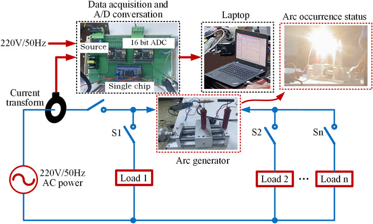
The overall structure of the arc experimental devices is shown in Figure 1, which is mainly composed of a 220V power frequency AC power supply, a current transformer, a load, an arc generator, a data acquisition module, and a computer. The arc generator is made according to the international UL1699 standard, including movable pointed copper electrodes, fixed flat graphite electrodes, insulating rods, metal slide rail bases, and stepper motors.

FIGURE 1

FIGURE 1. Circuit diagram of series arc experiment.

The experimental process is as follows: after the power supply and the load to be tested are turned on, the stepper motor is controlled to move the copper electrode to generate a stable combustion arc, the main circuit current is collected by the current transformer, and the AD7606 high-precision, 16-bit ADC and STM32 single-chip microcomputer are used to complete the analog-to-digital conversion and after data collection, upload fault and normal current data to a computer for further analysis. Considering the practical benefits, the sampling frequency of the current transformer should not be too high, and the lower frequency will cause the burial of the fault information, which will bring difficulties to arc identification. Taking a comprehensive consideration, 256 points are sampled per current cycle, that is, the sampling frequency is set to 12.8 kHz. According to the current waveform characteristics of the load, it can be divided into two types: linear and nonlinear loads. The current waveform of a linear load is an ideal sine wave, and the current waveform of a nonlinear load is a non-sinusoidal wave with periodic distortion. Considering the parallel use of loads and the difference in the location of the main circuit and branch circuit where the fault arc is located, the arc experimental scheme shown in Table 1 is designed.

TABLE 1

TABLE 1. Load types for arc experiments.

2.2 Characteristic analysis of fault arc current

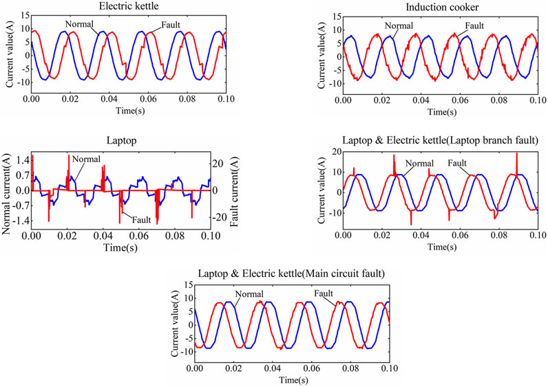
Figure 2 shows the current waveforms before and after the occurrence of arc faults measured under different loads. Due to the ionization of the air between the arc gaps, the molecular motion is intensified. According to electromagnetic theory, a large number of high-frequency pulse signals will be generated in the time-domain current signal. Since the generated random characteristics will be affected by external factors such as temperature, humidity, electrode material, etc., different current waveforms will be obtained in each experiment. After a series arc fault occurs in a purely resistive load, the current waveform appears to have ‘zero breaks’, and the symmetry of the positive and negative half cycles of the waveform decreases. Obvious random high-frequency signals appear in the fault waveform of eddy current loads. The normal waveform of the computer load is typically nonlinear.

FIGURE 2

FIGURE 2. Current waveforms before and after series arc fault.

Observing the normal and fault currents of each load, it is found that the nonlinear load will also produce an obvious ‘zero-break’ phenomenon during normal operation, which makes it easy to confuse the normal and fault states. The normal load and fault current spectrum of the kettle and the induction cooker are shown in Figure 3. It has been observed that the higher harmonics generated by a non-linear load (induction cooker) during normal operation are similar to those generated by a linear load (electric kettle) under fault conditions. To sum up, due to the existence of nonlinear loads such as switching power supplies, it is impossible to distinguish between normal and faulty states with a single feature in both the time and frequency domains.

FIGURE 3

FIGURE 3. Current spectrum before and after series arc fault.

3 Denoising autoencoder

3.1 Autoencoder

Autoencoder (AE) is a special neural network that can reconstruct the original input data through error backpropagation without supervision to automatically extract complex nonlinear features from the original input data. It has been widely used in intrusion detection, radiation source identification, picture, and video anomaly detection, and other fields.

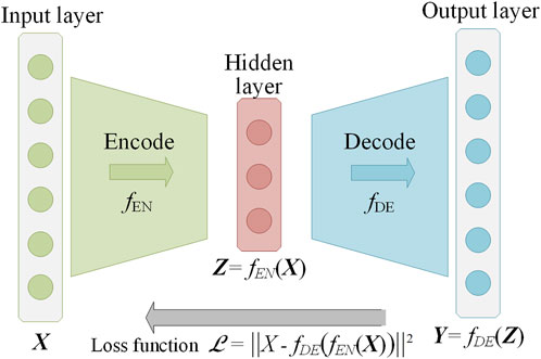
AE consists of an input layer, a hidden layer, and an output layer, which are connected by two neural networks: the encoder f_EN and the decoder f_DE, as shown in Figure 4. The input sample X of AE and the output reconstruction sample Y have the same dimension, while the dimension of the hidden layer data Z is generally smaller than the two. During training, AE first maps the input sample X to the hidden layer through the encoder f_EN to obtain its encoded feature value Z, as shown in Eq. 1.

$\mathbf{Z}=f_{EN}\left(\mathbf{{\rm X}}\right)=\sigma \left(\mathit{{\rm X}}\cdot {\mathit{W}}_{\mathit{E}\mathit{N}}+{\mathit{b}}_{\mathit{E}\mathit{N}}\right)(1)$

where is the encoder activation function, W_EN is the encoder weight matrix, and b_EN is the encoder bias.

FIGURE 4

FIGURE 4. Schematic diagram of autoencoder principle.

After the encoding is completed, the decoder f_DE is used to reconstruct the data of the hidden layer encoded feature Z, as shown in Eq. 2, W_DE and b_DE represent the activation function, weight matrix, and bias of the decoder, respectively.

$\mathit{Y}=f_{DE}\left(\mathit{Z}\right)=\delta \left(\mathit{Z}\cdot {\mathit{W}}_{\mathit{D}\mathit{E}}+{\mathit{b}}_{\mathit{D}\mathit{E}}\right)(2)$

The learning objective of AE is to minimize the deviation between the reconstructed sample Y and the original input sample X, which can be expressed as shown in Eq. 3.

$\mathbf{arg}\mathbf{min}\mathcal{L}\left(\mathit{Y},\mathit{X}\right)(3)$

When the reconstructed data of the autoencoder is different from the original input, it is necessary to use a loss function to formulate a penalty method. The commonly used mean square error loss function is shown in Eq. 4. The reduction of the reconstruction error needs to be achieved by gradient descent on the parameters W and b of the encoder and decoder.

$\mathcal{L}\left(\mathit{Y},\mathit{X}\right)={‖\mathit{X}-\mathit{Y}‖}_{\mathbf{2}}^{\mathbf{2}}(4)$

After the autoencoder is trained, the data contained in the hidden layer is the nonlinear feature extracted from the original input data.

3.2 Denoising autoencoder

For machine classification learning algorithms, if the input data contains unseparated noise and is considered a categorical feature of the data, it may cause overfitting of the classification algorithm, resulting in a decrease in the classification effect and generalization ability of the algorithm. The traditional AE can achieve better results after iterative training, but it cannot reduce noise, so a denoising autoencoder needs to be introduced to improve the generalization ability of the model.

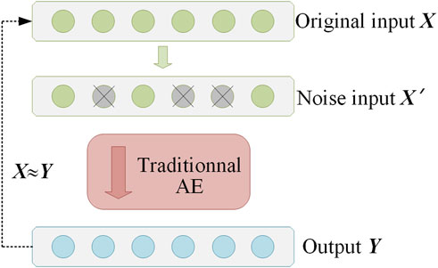
As shown in Figure 5, the denoising autoencoder is based on AE, adding random deactivation regularization to the input layer or by superimposing noise in the input samples as the input X′ of traditional AE. This paper chooses to implement DAE by superimposing noise in the original input, as shown in Eq. 5. The learning objective of DAE is to minimize the deviation between the reconstructed output sample Y and the original input X without superimposed noise.

$\left\{\begin{array}{c}{\mathit{X}}^{\prime }=\mathit{X}+{\mathit{N}}_{\mathit{F}}{\mathit{X}}_{\mathit{N}}\\ {\mathit{X}}_{\mathit{N}}\sim \mathit{N}\left(\mathbf{0},\mathbf{1}\right)\end{array}\right.(5)$

FIGURE 5

FIGURE 5. Principle of denoising autoencoder.

Among them, X′ is the original input data of superimposed noise, N_F is the noise superposition factor, and X_N obeys the standard normal distribution. After the above processing, the features learned by DAE from the input of superimposed noise are robust and can retain more relevant information in the latent space of the data, while filtering out irrelevant content such as noise.

4 Data preprocessing

4.1 Batch data acquisition and data normalization

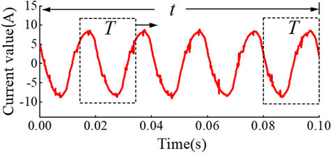
Since the normal or fault current signals obtained by the fault arc experiment have a large similarity in each cycle, if each cycle is an experimental sample, all the normal or fault samples of a single load have great similarity, and it is easy to cause the overfitting and generalization ability of the learned model to decrease. For this reason, this paper uses the sliding window to process the experimental data of the arc. While obtaining the batch data, it can not only capture the local features but also retain the time dependence of the time series data. The acquisition form is shown in Figure 6. The sliding window size T is a power frequency period, and the sampling frequency corresponding to this paper is 256 points. If the original data length is t, at most t-T+1 subsequence samples can be obtained.

FIGURE 6

FIGURE 6. Sliding window algorithm processing process.

4.2 Data normalization

Because the current values collected by different loads are quite different, the minimum value is less than 1A, and the maximum value can reach ten or even dozens of amperes. For neural networks and deep learning, if the value of a certain input dimension is high, it will cause the neural network to over-bias such features in learning, so it is necessary to standardize the data. Commonly used data standardization methods include maximum and minimum standardization, zero mean standardization, and maximum value standardization. This paper uses the maximum and minimum normalization to normalize the data, as shown in Eq. 6.

$x^{\prime }=\frac{x{-x}_{\mathit{min}}}{x_{\mathit{max}}-x_{\mathit{min}}}(6)$

Among them, x and x' are the sample data before and after normalization, respectively, and $x_{\mathit{max}}$ and $x_{\mathit{min}}$ are the maximum and minimum values of the sample, respectively. After the maximum and minimum normalization, the input current data of DAE is converted to a dimensionless value in [0,1], which avoids the influence of input volume during training of DAE and deep learning.

4.3 DAE feature extraction

The normal and fault current signals of each load are collected for five power frequency cycles. According to the sliding window data processing method above, 1,280–256 + 1 total of 1,025 samples can be obtained for each load’s normal and fault conditions. The cases correspond to 5,125 samples respectively, and the total number of samples is 10,250. Input the normalized sample data into DAE for training, and set the dimension of the hidden layer of DAE to 50, each sample can get 50-dimensional deep features with values between [0, 1], and expand it to [0, 255] In the interval, the characteristic grayscale images corresponding to normal conditions and arc faults can be drawn, as shown in Figure 7.

FIGURE 7

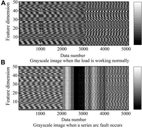
FIGURE 7. Grayscale images before and after a series arc fault. (A) Grayscale image when the load is working normally; (B) Grayscale image when a series are fault occurs.

5 Deep residual network fault identification

Computer vision recognition is similar to the visual sense of the human eye, and its ability to distinguish color images is much higher than that of grayscale images. In order to extract more arc fault features from the feature map, the grayscale images obtained are image-enhanced with false colors. Input the grayscale image into the three primary color channels of red, green, and blue (RGB) with different changing characteristics, and then synthesize the RGB values output by each channel to obtain the pseudo-color image corresponding to the grayscale image, as shown in Figure 8.

FIGURE 8

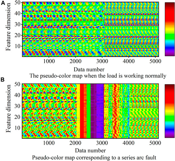
FIGURE 8. Pseudo-color images before and after arc fault. (A) The pseudo-color map when the load is working normally; (B) Pseudo-color map corresponding to a series arc fault.

5.1 Convolutional neural network

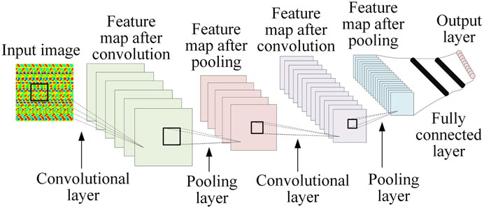
Convolutional Neural Network (CNN) is a representative method in deep learning. It is constructed by imitating the biological vision mechanism and has a good representation of learning ability. Two-dimensional CNN is often used in the field of computer vision (CV) and image processing. It contains two dimensions, height, and width, and extracts image features through multi-layer convolution operations. A typical CNN consists of convolutional layers, pooling layers, and fully connected layers, as shown in Figure 9.

FIGURE 9

FIGURE 9. Typical 2D CNN structure diagram.

The convolutional layer is used to extract local features. First, the inner product of the overlapping part of the input layer data information and the two-dimensional convolution kernel is calculated, and then the feature output value is obtained by passing it through a nonlinear activation function, as shown in Eq. 7. As shown, the activation function usually adopts a rectified linear unit (ReLU), which can clear the output of some neurons to speed up the training speed.

${\mathit{x}}_{\mathit{i}}^{\mathit{k}}=\mathit{g}\left({\mathit{w}}_{\mathit{i}}^{\mathit{k}}*{\mathit{X}}^{\mathit{k}-\mathbf{1}}+{\mathit{b}}_{\mathit{i}}^{\mathit{k}}\right)(7)$

Among them, ${\mathit{x}}_{\mathit{i}}^{\mathit{k}}$ is the ith feature map of the kth layer; ${\mathit{w}}_{\mathit{i}}^{\mathit{k}}$ is the ith convolution kernel matrix of the kth layer; ${\mathit{X}}^{\mathit{k}-\mathbf{1}}$ is the output of the kth layer of the network; $b_i^k$ is the kth layer convolutional layer the bias value of; g ($\cdot$) is the ReLU activation function, and the expression is as shown in Eq. 8.

$\left\{\begin{array}{c}\mathbf{ReLU}\left(\mathit{x}\right)=\mathit{max}\left(\mathbf{0},\mathit{x}\right)\\ \mathit{x}\in \left(-\mathit{\infty },+\mathit{\infty }\right)\end{array}\right.(8)$

The pooling layer is located after the convolution layer and has two main functions. One is to reduce the dimension of the extracted high-dimensional features to improve the operation efficiency and avoid overfitting; the other is to ensure the invariance of the features and improve the generalization ability of the model.

${\mathit{Y}}_{\left(\mathit{i},\mathit{j}\right)}^{\mathit{k}}={\mathit{p}\mathit{o}\mathit{o}\mathit{l}}_{\left(\mathit{m},\mathit{n}\right)\in {\mathit{R}}_{\mathit{i},\mathit{j}}}\left({\mathit{X}}_{\left(\mathit{m},\mathit{n}\right)}^{\mathit{k}-\mathbf{1}}\right)(9)$

In Eq. 9, $Y_{\left(i,j\right)}^k$ is the value of the kth pooling layer at (i, j); pool ($\cdot$) represents the pooling rules, including maximum pooling, random pooling, and average pooling; $R_{i,j}$ is the receptive field at (i, j); $X_{\left(m,n\right)}^{k-1}$ is the corresponding input at the receptive field (m, n). After the convolution and pooling processing, the features of the pooling layer are further extracted by the fully connected layer to output the model results. Finally, the normalized exponential function Softmax is used to complete the multi-classification task of the data.

5.2 Deep residual networks

The typical methods of deep learning cannot reflect its “depth”. When the network depth is deepened, the gradient will gradually disappear in the backpropagation. In addition, deep learning still has the problem of degradation. With the deepening of the network accumulation layer, its performance begins to decline, resulting in the performance of the shallow networks being better than that of the deep networks. The error of the degenerate network on both the training set and the test set is high, which shows that the degradation problem is not caused by overfitting.

To solve the problem of gradient disappearance in deep learning, and hope to increase the number of network layers and also improve the accuracy of the model, based on the architecture of CNN, He et al. (He et al., 2016) proposed a deep residual network. ResNet learns from the cross-layer connection idea of a high-speed network and introduces residual building block (RBB), skips the convolution block through shortcut connection to avoid gradient disappearance, and makes the input X of the neural network pass through identity mapping $\lambda$: X $\to$ X is short-circuited to the output Y of the parameterized layer, and the parameterized layer gets the corresponding residual map f: X $\to$ Y-X.

The residual block structure is shown in Figure 10, CONV represents the convolutional layer. BN represents de-mean normalization to reduce the difference between different features. The left and right pictures are the standard residual block and the residual block with the downsampling layer, respectively. Compared with CNN, the parameterized layer learns the direct mapping between input and output f: X $\to$ Y, and learns the residual mapping f: X $\to$ Y-X of the two can effectively reduce the difficulty of network learning, breaking the convention that the output of the nth layer of the traditional neural network can only be used as the input of the n+1st layer. By constructing the residual network, the training depth of ResNet can reach hundreds or thousands of layers, and the network performance will not be degraded.

FIGURE 10

FIGURE 10. Residual block structure diagram in ResNet.

5.3 ResNet network training and testing results

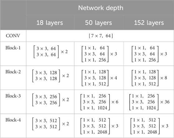
After extracting the normal and fault arc features using the previous data processing method and DAE, a total of 10,250 samples were obtained, of which 8,000 samples were used as the training set of ResNet, and 2,250 samples were used as the test set. Each sample is a 1 × 50-dimensional RGB three primary color image, which is cut and reorganized into 5 × 10-dimensional, and then the 5 × 10-dimensional graphics of three RGB channels are used as the input of ResNet. The network learning depth of ResNet is set to 18, 50, and 152 layers respectively (referring to the convolution layer and the fully connected layer, excluding the pooling layer), and its structure deployment is shown in Table 2, where Block represents a residual block with three convolutional layers. The computational costs of ResNet with different depths are shown in Table 3.

TABLE 2

TABLE 2. The network structure of ResNet.

TABLE 3

TABLE 3. The computational cost of ResNet.

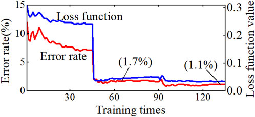
When the training depth of ResNet is 18 layers, the error rate and network loss function value of the model on the test set are shown in Figure 11. It is observed that both the network error rate and the network loss function value gradually decrease with the increase in training times. When the training times reach 60, the correct rate of ResNet judging the series arc fault is over 98%. Increasing the number of model training, and when the training reaches about 120, the fault identification accuracy rate increases to 98.9%. It can be seen that the error rate of network judgment is still decreasing when the number of model training is increased, but the convergence speed is relatively slow at this time.

FIGURE 11

FIGURE 11. ResNet error rate and loss function value.

At different training depths of 18, 50, and 152, the error rates of ResNet on the training and test sets are shown in Figure 12. The batch size of the dataset used for training (BatchSize) is 50, which means that there are 50 groups of data involved in each training. Epoch is used to represent the number of traversal training for all data. For 1 Epoch, the training set and test set correspond to 160 and 45 iterations, respectively. Observing Figure 12, it is found that the error rate decreases significantly at each Epoch, and when the number of training reaches about 400, the correct rate of the training set under the three training depths is all higher than 98.9%. When the training depth is 152, the training set accuracy rate is the highest, reaching 99.5%. On the test set, the correct rates of ResNet with training depths of 18, 50, and 152 reached 98.9%, 99.3%, and 99.7%, respectively, and the super-high-level ResNet with 152 layers had the highest correct rate. By increasing the number of training sessions at each depth, the accuracy no longer improves significantly but converges to the aforementioned values. It can be seen that even if the training depth of ResNet has reached the super-high level of 152, its accuracy on the training set and test set can be gradually improved, and there is no degradation of deep learning.

FIGURE 12

FIGURE 12. The error rate on the training set and test set.

5.4 Generalization ability test of DAE-ResNet

Considering the variety of loads in practice, it is difficult to take into account all possible loads in deep learning training. In this regard, the training set and test set are adjusted as follows and ResNet is retrained: keep the previous processing methods such as DAE, sliding window, and pseudo-color processing unchanged, so that the training set only contains the loads numbered 1,2,4, and five in Table 1; the test set only contains the load numbered three in Table 1. In short, the load of the test set does not participate in the network training of ResNet at all to examine the generalization ability of the DAE-ResNet method to the load outside the training.

After the above dataset is adjusted and the model is retrained, the training results of ResNet on the training set and test set are shown in Figure 13. It has been observed that when the load does not participate in network training but participates in network testing, ResNet has a very high accuracy rate on the training set, and the accuracy rate reaches and converges to 100% after 320 training sessions. Although the performance on the test set is not as good as the training set, after about 100 training sessions, ResNet with a training depth of 152 can still reach and converge to a fault recognition rate of 97.6%. It can be seen that the DAE-ResNet method still has a high fault recognition rate for loads other than the training set, has strong generalization ability for different loads, and has good performance in practical applications.

FIGURE 13

FIGURE 13. Recognition rate of loads not involved in training.

The method in this paper is compared with existing support vector machine (SVM), support vector machines optimized by particle swarm optimization (PSO-SVM), neural networks optimized by particle swarm optimization (PSO-BP), random forests (RF), and convolutional neural networks. Among them, SVM adopts radial basis kernel function, BP is set to four layers, and the maximum depth of RF is 5. The time-domain features used include current kurtosis, higher-order cumulant, current variance, and the current rate of change, and the frequency-domain features include harmonic factor, total harmonic distortion rate, frequency centroid, and sub-band energy ratio, and the wavelet transform is used in the time-frequency domain to analysis and extract its wavelet entropy. Each recognition method is tested in the two situations above: one is that each load is included in the training set, and the other is that the load to which the test set belongs is not included in the training set. The recognition results of each arc detection method are shown in Table 4. The BNN method has a better recognition rate in the common training mode, but when the load of the test set does not participate in the network training, the fault recognition rate is low. The fault recognition rate of the method in this paper is better than other types of recognition methods in both cases, and it also has a good generalization ability for untrained loads.

TABLE 4

TABLE 4. Comparison of different arc identification methods.

6 Conclusion

Most of the existing arc identification methods are based on the time-frequency domain characteristics of arc current. Due to the subjectivity of manually extracting arc fault characteristics, it is impossible to reveal the deeper characteristics of fault arcs. Using current data as input to deep learning algorithms has the problem of insufficient feature extraction. In this regard, this paper uses DAE combined with ResNet to identify series arc faults:

1) The sliding window is used to obtain batch samples from the normal and fault arc signals obtained in the experiment, which effectively avoids the overfitting and reduced generalization ability of the deep learning algorithm caused by the similarity of the samples. And normalize them to avoid the feature bias caused by the deep learning network over-biasing such features in learning due to the high value of a certain input dimension.

2) The powerful feature self-extraction ability of denoising autoencoders is used to extract high-dimensional abstract features from normal and fault arc current signals. The time-frequency domain features of fault arc current are no longer used, and the subjectivity of manual feature extraction is avoided.

3) Convert the feature values obtained by DAE into grayscale images. Since deep learning has a high resolution for image color, the grayscale image is processed with pseudo-color to generate an RGB three-channel pseudo-color image, and the three-channel image is used as the input of the deep learning network. They are input to ResNet networks of different depths for training. The recognition rate of ResNet at different network depths is above 98.9%, and the arc recognition rate reaches 99.7% at a super high-level depth of 152 layers. For loads that do not participate in ResNet network training, the recognition rate can also reach 97.6%, showing good generalization ability.

4) The method in this article is combined with the existing support vector machine (SVM), support vector machine optimized by particle swarm algorithm (PSO-SVM), neural network optimized by particle swarm algorithm (PSO-BP), random forest (RF), and convolutional neural network. Identification methods for comparison. The fault identification rate of this method is better than other types of identification methods in both cases when each load is included in the training set and when the load in the test set is not included in the training set, and it also has good generalization ability for untrained loads.

7 Prospect

As people pay more attention to electrical fires, arc fault detection technology has received more and more attention from the country and industry. This paper proposes a series fault arc detection method based on denoising autoencoders (DAE) and deep residual networks (ResNet). It avoids the subjectivity problem of manual extraction of arc fault features and uses a deep residual network to more comprehensively extract deep fault features from fault feature images. However, there are still many challenges worthy of further research for practical applications. Here is a brief prospect:

1) Since there is no public data set of arc fault, this paper used a self-built data set in the research. However, the lack of an authoritative public data set has a huge impact on the research, comparison, and application of arc fault detection technology.

2) Although the practicality of the model has been taken into account during the design process and the computational complexity of the model has been reduced as much as possible by controlling the network scale, the network model proposed in this article still requires a relatively large amount of calculations and requires high computing power of the MCU in the circuit protection device.

3) The current research on arc fault detection technology is based on the research of a single detection point. However, in actual scenarios, many lines are interconnected and contain multiple detection points. How to synthesize the information of these detection points to improve the overall accuracy of series arc fault detection will be a very meaningful research direction.

Data availability statement

The original contributions presented in the study are included in the article/Supplementary Material, further inquiries can be directed to the corresponding author.

Author contributions

JW: Writing–review and editing. XL: Writing–original draft. YZ: Writing–original draft, Data curation, Methodology.

Funding

The author(s) declare that no financial support was received for the research, authorship, and/or publication of this article.

Conflict of interest

The authors declare that the research was conducted in the absence of any commercial or financial relationships that could be construed as a potential conflict of interest.

Publisher’s note

All claims expressed in this article are solely those of the authors and do not necessarily represent those of their affiliated organizations, or those of the publisher, the editors and the reviewers. Any product that may be evaluated in this article, or claim that may be made by its manufacturer, is not guaranteed or endorsed by the publisher.

Supplementary material

The Supplementary Material for this article can be found online at: https://www.frontiersin.org/articles/10.3389/fenrg.2024.1341281/full#supplementary-material

References

Bao, G. H., and Jiang, R. (2019). Research on series arc fault detection based on the asymmetrical distribution of magnetic flux. Chin. J. Sci. Instrum. 40, 54–61. doi:10.19650/j.cnki.cjsi.J1804570

CrossRef Full Text | Google Scholar

Charles, J. K. (2009). Electromagnetic radiation behavior of low-voltage arcing fault. IEEE Trans. Power Del. 24, 416–423. doi:10.1109/TPWRD.2008.2002873

CrossRef Full Text | Google Scholar

Chu, R. B., Zhang, R. C., Yang, K., and Xiao, J. C. (2020). Series arc fault detection method based on multi-layer convolutional neural network. Power Syst. Technol., 4792–4798. doi:10.13335/j.1000-3673.pst.2019.2489

CrossRef Full Text | Google Scholar

Cui, R. H., Tong, D. S., and Li, Z. (2021). Aviation arc fault detection based on generalized S transform. Proc. Chin. Soc. Electr. Eng. 41, 8241–8250. doi:10.13334/j.0258-8013.pcsee.201626

CrossRef Full Text | Google Scholar

Gong, Q., Peng, K., Wang, W., Xu, B., Zhang, X., and Chen, Y. (2022). Series Arc fault identification method based on multi-feature fusion. Front. Energy Res. 9, 824414. doi:10.3389/fenrg.2021.824414

CrossRef Full Text | Google Scholar

He, K. M., Zhang, X. Y., Ren, S. Q., and Sun, J. (2016). “Deep residual learning for image recognition,” in Proceedings of 2016 IEEE Conference on Computer Vision and Pattern Recognition(CVPR), Las Vegas, NV, USA, 27-30 June 2016, 770–778. doi:10.1109/cvpr.2016.90

CrossRef Full Text | Google Scholar

Jiang, J., Li, W., Li, B., Ma, J. T., and Zhang, C. H. (2022). Application of the Hurst index of current frequency spectrum in series arc fault detection. Control Theory and Appl. 39, 561–569. doi:10.7641/CTA.2021.10670

CrossRef Full Text | Google Scholar

Liu, G. F., and Li, Y. (2019). Arc fault recognition method of genetic algorithm optimized GMM. Meas. Control Technol., 77–81. doi:10.19708/j.ckjs.2019.01.016

CrossRef Full Text | Google Scholar

Liu, G. G., Du, S. H., Su, J., and Han, X. H. (2017). Research on LV arc fault protection and its development trends. Power. sys. techno. 41, 305–313. doi:10.13335/j.1000-3673.pst.2016.0804

CrossRef Full Text | Google Scholar

Long, G. W., Mu, H. B., Zhang, D. N., Li, Y., and Zhang, G. J. (2021). Series arc fault identification technology based on multi-feature fusion neural network. High. Volt. Eng., 463–471. doi:10.13336/j.1003-6520.hve.20200336

CrossRef Full Text | Google Scholar

Lu, Q. W., Wang, T., Li, Z. R., and Wang, C. (2017). Detection method of series arcing fault based on wavelet transform and singular value decomposition. Trans. China Electrotech. Soc., 208–217. doi:10.19595/j.cnki.1000-6753.tces.170196

CrossRef Full Text | Google Scholar

Qu, N., Zuo, J. K., Chen, J. T., and Li, Z. Z. (2019). Series arc fault detection of indoor power distribution system based on LVQ-NN and PSO-SVM. IEEE Access 7, 184020–184028. doi:10.1109/ACCESS.2019.2960512

CrossRef Full Text | Google Scholar

Wang, Y., Luo, Z. Q., Li, S. N., Chen, T., Hou, X. Z., and Fu, X. Y. (2022). Series fault arc identification based on time-frequency chromatogram. Appl. Electron. Tech., 70–75. doi:10.16157/j.issn.0258-7998.212349

CrossRef Full Text | Google Scholar

Wang, Y., Zhang, F., and Zhang, S. (2018). A new methodology for identifying arc fault by sparse representation and neural network. IEEE Trans. Instrum. Meas. 67, 2526–2537. doi:10.1109/TIM.2018.2826878

CrossRef Full Text | Google Scholar

Yang, K., Zhang, R. C., Yang, J. H., Du, J. H., Cheng, S. H., and Tu, R. (2016). Series arc fault diagnostic method based on fractal dimension and support vector machine. Trans. China Electrotech. Soc. 31, 70–77. doi:10.19595/j.cnki.1000-6753.tces.2016.02.010

CrossRef Full Text | Google Scholar

Yu, Q. F., Huang, G. L., Yang, Y., and Sun, Y. Z. (2019). Series fault arc detection method based on AlexNet deep learning network. J. Electron. Meas. Instrum., 145–152. doi:10.13382/j.jemi.B1801800

CrossRef Full Text | Google Scholar

Zhao, H. J., Qin, H. Y., Liu, K., and Zhu, L. J. (2020). Series fault arc detection method based on relevant theories and zero break feature fusion. Chin. J. Sci. Instrum. 218–228. doi:10.19650/j.cnki.cjsi.J2006019

CrossRef Full Text | Google Scholar