Exploring quantum learning in the smart grid through the evolution of noisy finite fourier series

The decentralization and softwarization of modern industrial control systems such as the electric grid has resulted in greater efficiency, stability and reliability but these advantages come at a price of higher likelihood of cyberattacks due to the resulting increase in cyberattack surface. Traditional cyberattack detection techniques such as rule-based anomaly detection have an important role to play in first response. However, given the data-rich environment of the modern electric grid, current research thrusts are focused on integrating data-driven machine learning techniques that automatically learn to detect anomalous modes of operation and predict the presence of new attacks. Quantum machine learning (QML) is a subset of machine learning that aims to leverage quantum computers to obtain a learning advantage by means of a training speed-up, data-efficiency, or other form of performance benefit. Questions remain regarding the practical advantages of QML, with the vast majority of existing literature pointing to its greater utility when applied to quantum data rather than classical data, which within a smart grid environment include TCP/IP packets or telemetry measurements. In this paper, we explore a scenario where quantum data may arise in the smart grid, and exploit a quantum algorithmic primitive previously proposed in the literature to demonstrate that in the best-case, QML can provide accuracy advantages of $>25$ percentage points when predicting anomalies.

1 Introduction

The cyber-enabled power grid, known as the smart grid, is characterized, in part, by its greater dependence on computing enabling new forms of power system analytics. As such, data has become the epicentre of decision-making in this (and other) critical infrastructures. Over the last 15 years, the transformation of the power grid to a more information and communication technology (ICT)-rich environment has had broad implications enabling a more adaptable, sustainable and consumer-centric power generation, transmission and delivery system while increasing its vulnerabilities to cyberattacks. The December 2015 and 2016 cyberattacks on the Ukrainian power grid as well as the May 2021 cyberattack on the U.S. colonial pipeline have demonstrated the damage and devastation, that is, possible when malware infiltrates critical infrastructure, that is, growingly dependent on ICT.

Traditional cybersecurity techniques such as rule-based cyberattack detection have an important role to play in protecting the smart grid; however, history has taught us that these manually designed controls are insufficient to account for all the possible ways that an attacker can infiltrate the system especially when it comes to recognizing novel attack signatures. Data-driven machine learning techniques are under investigation and implementation as a possible first line of defense against cyberattacks given their propensity to model complex relationships (not easily described through explicit rules) to automatically discover (new) cyberattack patterns and anomalous modes of operation. Machine learning for the security of general cyber-physical systems (Lukens et al., 2022) as well the more specific security of the smart grid is an active area of research (Ashrafuzzaman et al., 2020; Karimipour et al., 2019; Khaw et al., 2020; Jahromi et al., 2020, Jahromi et al., 2021; Zhang et al. 2021) that has already shown promising results. The authors in Ashrafuzzaman et al. (2020) develop an ensemble technique that can classify different kinds of cyberattacks; the technique works well, but there is potential for improvement in the case of very heavily imbalanced data. The works in Karimipour et al. (2019); Khaw et al. (2020); Jahromi et al. (2020), Jahromi et al., (2021); Irfan et al. (2023), on the other hand, make use of unsupervised anomaly detection methods such as autoencoders and Boltzmann machines that cannot classify different kinds of cyberattacks, but handle data imbalance better because they train on normal and not cyberattack data. Zhang et al. (2021) provides a good survey of techniques for anomaly detection in smart grid time-series data, including a section on possible future directions such as transfer learning (Niu et al., 2020), a technique that fine-tunes models trained on different but closely related tasks to achieve data efficiency, and the use of generative adversarial networks (Creswell et al., 2018) to generate realistic synthetic data(Luo et al., 2018; Zhang et al., 2020). The authors in Irfan et al. (2023) provide a very recent survey specifically related to the detection of FDI attacks, and touch on important topics such as the localization of these attacks in addition to their detection.

Concurrently, the recent rise of quantum computers and quantum information processing devices (Nielsen and Chuang, 2002) that can outperform classical computers in tasks such as cryptographic code-breaking (Gisin et al., 2002; Pirandola et al., 2020) and simulation of quantum dynamics (Brown et al., 2010) has naturally led to questions as to whether quantum computers may be useful for machine learning. This is, again, an active area of research with some work specifically focusing on the application of quantum machine learning in smart grids (Zhou and Zhang, 2021; Ullah et al., 2022), but thus far, existing results in the literature have been a mixed bag. The first era of quantum machine learning aimed to provide exponential speedups to machine learning algorithms that make heavy use of Linear Algebra by performing the linear algebraic subroutines in logarithmic time instead of polynomial time (Harrow et al., 2009; Kerenidis and Prakash, 2016; Lloyd et al., 2013) as is typical for classical machine learning. However, the theoretical speedups afforded by these algorithms required that the input data would be provided in the form of a quantum state. If one accounts for the time needed to transform classical data to a quantum state, and also allows classical machine learning algorithms to exploit data preparation assumptions that have a similar time complexity, the apparent exponential speedup advantage disappears (Tang, 2019; Chia et al., 2020). There have also been quantum algorithms that provide small polynomial speedups (most commonly a quadratic speedup) to machine learning problems (Harrow, 2020); however, it is doubtful that these theoretical speedups will hold in practice because of the error correction overhead needed to engineer a fault tolerant quantum computer (Babbush et al., 2021). Quantum annealing (Albash and Lidar, 2018) is another proposed quantum algorithm that relies on a correspondence between finding the ground energy of a physical system and minimizing an optimization problem, although there is again no guaranteed practical advantage (Crosson and Lidar, 2021). The situation is a lot more promising when one restricts themselves to quantum data, which is data, that is, naturally already given as a quantum state. An example may be data which is captured by a quantum sensor (Degen et al., 2017), which then transduces a quantum state vector directly into the quantum computer for learning for which exponential advantages have been proven (Huang et al., 2021a).

Quantum sensors show promise in a wide variety of domains ranging from improved cancer detection to improved geological exploration, although their application in a smart grid context remains an under-explored area of research. The general expectation is that the availability of this data in a real-world scenario lies in the medium to long term. However, the exciting possibilities offered by quantum data leads us to take a proactive approach and through academic-power utility collaboration propose a preliminary scenario for how it may arise in the smart grid. After proposing a viable scenario, we generate appropriate synthetic quantum data and study quantum learning advantages. The studies performed on this synthetic data aim to highlight general principles and are not expected to perfectly translate to imminent results obtained on real-world smart grid quantum data when it becomes available. Through this first step, we aim to define a scenario which can then be progressively refined in subsequent work as the future of quantum data in smart grid unfolds.

The rest of this paper is organized as follows: given that an intended audiences of this paper are smart grid researchers or professionals who may not be familiar with quantum computing, we first briefly introduce the topic and explain why quantum machine learning for classical data can be problematic in Section 2. Next, we define the quantum data scenario in Section 3, and then formulate the problem and explain how we can incorporate a previously proposed algorithm in the theoretical quantum machine learning literature that “rigs” datasets to show a quantum advantage within our proposed smart grid quantum anomaly detection framework in Section 4 and Section 5. The main contribution of this paper is presented in Section 6, where we propose a differential evolution algorithm that can be used to generate noisy finite Fourier series that exhibit a large quantum advantage. We then show that quantum machine learning can achieve a stunning $>25$ percentage points advantage in accuracy on the generated datasets in Section 7, and conclude highlighting potential future work and improvements in Section 8.

2 The case for QML for quantum data

At a simple level, quantum mechanics can be thought of as an alternative to classical probability theory (Aaronson, 2004), with a quantum state vector being different in two mains ways from a classical probabilistic vector:

1. Regular probabilities that fall between 0 and 1 are replaced with probability amplitudes that can, in general, be complex numbers.

2. Regular probability theory requires that the ℓ¹ norm of the probability vector under consideration be conserved under transformation, which implies that a valid classical probabilistic evolution consists of repeated multiplications by stochastic matrices. Quantum mechanics requires that the ℓ² norm of the probability amplitude under consideration be conserved, which instead intimates that a valid quantum evolution consists of repeated multiplications by unitary matrices. The only exceptions are the measurements at the end of the evolution which define the statistics of the observations.

If one has two quantum state vectors $\psi \in {\mathbb{R}}^{2^n},\varphi \in {\mathbb{R}}^{2^m}$, then their joint vector is described by the vector $\zeta \in {\mathbb{R}}^{2^n}\otimes {\mathbb{R}}^{2^m}$ obtained from the tensor product ζ = ψ ⊗ ϕ.

Quantum computing uses quantum state vectors and their evolutions to define quantum analogues to elements of the familiar circuit model of computing:

1. Bits are replaced by qubits; these are realized by any object which is physically described by a two-dimensional quantum state vector (for example, the polarizations of a photon). Usually, all qubits are initialized to objects described by the blank state |0⟩:= [1,0]^⊤ at the start of a computation. The joint space of n blank qubits is described by the vector ${\otimes }_{i=1}^n|0\rangle$.

2. Logic gates are replaced by quantum gates, which are the unitary transformations acting on the state vector of a collection of qubits. Usually, these gates are restricted to act on one or two qubits only. Note that after the application of some quantum gates on n blank qubits, it may no longer be possible to write the joint state vector as the tensor product of n two-dimensional quantum state vectors. This is a fundamental phenomenon called entanglement, and it is the reason why large quantum computations cannot be easily simulated on a classical computer.

3. A collection of qubits are measured at the end of a circuit. This measurement is simply a probabilistic operation that returns a collection of classical bits.

The small changes to the standard circuit model of computation result in a surprisingly more powerful theory from the point of view of computational complexity theory, with quantum algorithms being able to solve problems such as prime factorization in polynomial time (Shor, 1999), while classical computers are widely believed to take exponential time.

Because of the recent explosion surrounding machine learning, it is natural to consider whether quantum algorithms can provide an advantage to learning problems. As mentioned in Section 1, there are many ways of tackling this question, such as through the use of linear algebraic algorithms that make use of quantum circuits in some way. However, the two algorithms that are most straightforward to relate to classical machine learning approaches are quantum neural networks (Benedetti et al., 2019) and quantum SVMs (Schuld and Killoran, 2019). A quantum SVM is simply a regular SVM that makes use of a quantum circuit as part of its feature map, and a quantum neural network is simply a regular neural network with a (fixed or parametrized) quantum circuit as part of its layers. A parametrized quantum circuit is one in which one of the quantum gates is dependent on a parameter. For example, a valid one-qubit gate involves rotation about the x-axis; here, the gate’s rotation angle can represent the parameter, that is, adjusted (through the use of gradient descent) for learning. We also note that a quantum neural network may have all quantum layers without any classical layers.

However, as mentioned in Section 1, QML for classical data (i.e., data that does not naturally take the form of a quantum state vector) can be problematic. We provide intuition as to why this is the case by highlighting two factors:

1. Quantum information is fragile, especially when compared with classical. The state vector represented by quantum qubits decoheres (i.e., collapses into a classical state vector) quickly, which implies that quantum error correction to mitigate this decoherence is essential. Previous studies have shown that quantum error correction algorithms impose a large constant overhead on quantum algorithms (Babbush et al., 2021).

2. When subjected to rigorous theoretical analysis, the vast majority of practically useful QML for classical data algorithms only offer a small polynomial speedup compared to their classical machine learning counterparts. For example, a QML algorithm might have to conduct O(n) operations whereas the classical machine learning algorithm would have to execute O(n²) operations, with n being the size of the data input. Even quantum algorithms which were previously thought to offer exponential advantages for big classical data were later shown to only offer polynomial advantages if one removes some unrealistic data loading assumptions (Chia et al., 2020; Tang, 2019, Tang, 2021).

One may argue that small polynomial speedups are still useful speedups, but the problem is that the big O notation neglects the constant overhead. As an example, an algorithm that requires 2n operations to complete and an algorithm that takes 10⁸n operations to finish would both be denoted O(n). Moreover, big O notation, which is concerned with asymptotic limits (as n → ∞) suggests that an algorithm which takes 10⁸n operations to finish would be superior in terms of complexity to an algorithm that takes n² operations. However, in the practical world, say n ∈ [0, 10⁷]; here, n² operations are at least an order of magnitude lower than 10⁸n, even though n can be large. It is possible to argue that for sufficiently large data sets, 10⁸n operations are lower complexity than n². While this is true, for an n of this size, 10⁸n itself may be infeasible albeit it is better than n².

QML for classical data suffers from the challenge described above because of the large constant overhead imposed by quantum error correction and the fact that the vast majority of proposed algorithms only offer small polynomial speedups. If n is large enough to make QML more attractive than classical ML, we argue that the QML algorithm itself will likely also be impractically slow. QML for quantum data, however, does not suffer from this problem, since it can offer exponential advantages over classical ML for quantum data. We note that there is an important caveat here: not all quantum datasets offer exponential advantages for quantum data, even though the advantage is likely to occur.

At the heart of the quantum versus classical debate is the notion of “value for investment”, and this holds for QML for quantum data too. Quantum systems, undoubtedly, pose additional challenges such as infrastructural costs. However, one must look at the larger picture. When a quantum system promises a potential exponential advantage, it is not just discussing a slight edge or a quicker solution, it is about turning otherwise infeasible problems into achievable tasks. For example, the accurate analysis of quantum data collected from quantum infrastructure in a future smart grid could provide better cyberattack detection performance, better and cheaper maintenance, and faster reponses to outages. In such scenarios, the “cost” of quantum computing, both financial and computational, becomes a necessary investment in order to ensure optimal grid operations.

3 Smart grid quantum anomaly detection scenarios

The effect of quantum technology on the smart grid remains to be seen, but one can reasonably conclude that devices like quantum sensors (Degen et al., 2017; Crawford et al., 2021) are likely to play a pivotal future role given their increased sensitivity and performance. We assert that defining a general, relatively unconstrained framework for studying the effects of quantum technology on the grid is a valuable approach to shed tangible insights as the field develops.

It is desirable to enlist within our framework select facets of the current smart grid infrastructure to ground the model in real world characteristics. One such aspect is the prevalence of periodicity in classical Operational Technology (OT) data: current classical grid infrastructure is comprised of periodic waveforms (such as time-dependent voltage and current readings) stemming from the alternating current (AC) nature of the power grid backbone. Given the prohibitive cost of completely replacing legacy AC power grid components, this periodic characteristic of signals is likely to hold in a quantum-enabled future smart grid. Hence, we aim to incorporate information periodicity in our proposed anomaly detection scenario.

An example of a potential scenario is shown in Figure 1, which presents an interaction between a generic real-time current/voltage measurement device (RTMD), which outputs samples from noisy periodic waveforms, and envisioned future quantum infrastructure. The measurements of the RTMD, in accordance with practical measurement devices, are distorted by some level of noise. Since currents and voltages are sinusoidal in nature, the RTMD outputs a noisy periodic waveform; this waveform is sampled and fed as a control signal to a quantum device. A simple cyberattack scenario is one in which the attacker compromises the RTMD and causes it to output anomalous samples that are classically difficult to differentiate from the regular noisy samples and which cause the quantum device to malfunction. By classically difficult, we mean that a function which effectively differentiates a regular noisy signal from anomalous samples must necessarily be quantum in nature. Based on our discussions above, this could be modeled as inputting the noisy/anomalous signal in question into quantum infrastructure in some way and then inferring based on outputs from that infrastructure. Specifically, if we let $q(x):{\mathbb{R}}^u\to {\mathbb{R}}^m$ be the function that describes the dynamics of the quantum infrastructure, then differentiating between noisy or anomalous signals requires learning some function $a(q(p)):{\mathbb{R}}^u\to \{\text{normal\hspace{0.17em},\hspace{0.17em}FDI}\}$. Such a scenario lends itself to the availability of quantum data within smart grid infrastructure; such data depends on the behaviour of the theoretical quantum infrastructure. In practice, the attacker can either target the physical dynamics of the device generating the waveform or the sampling device directly. Given that quantum smart grid infrastructure does not currently exist making it difficult to form specific assumptions as in the classical infrastructure case, we simply assume that it can produce useful quantum state vectors through the use of entangled operations. We assert that this fundamental condition is likely to be satisfied by all useful quantum devices since non-entangled operations can be efficiently simulated on classical devices.

FIGURE 1

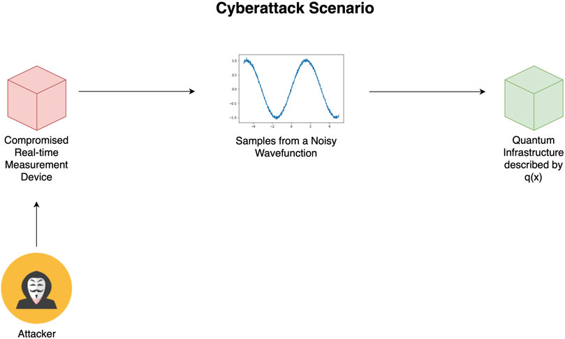
FIGURE 1. An example of the proposed cyberattack structure of a future hybrid quantum-classical smart grid. The cyberattack scenario occurs when an attacker compromises the real-time measurement device and causes it to output anomalous false data that cause the quantum device to malfunction, with the anomalies being classically difficult to differentiate from the regular noisy samples.

Hence, the goal is to train a machine learning algorithm to distinguish between noisy or anomalous samples arising from a compromised RTMD, which is illustrated in Figure 2. Given the focus on quantum data, we assert that it is likely that a quantum machine learning supervisor results in exponentially better cyberattack detection than a classical counterpart. In this paper, we explore the potential of QML in this context through the evolution of random Fourier functions as discussed in Section 6.

FIGURE 2

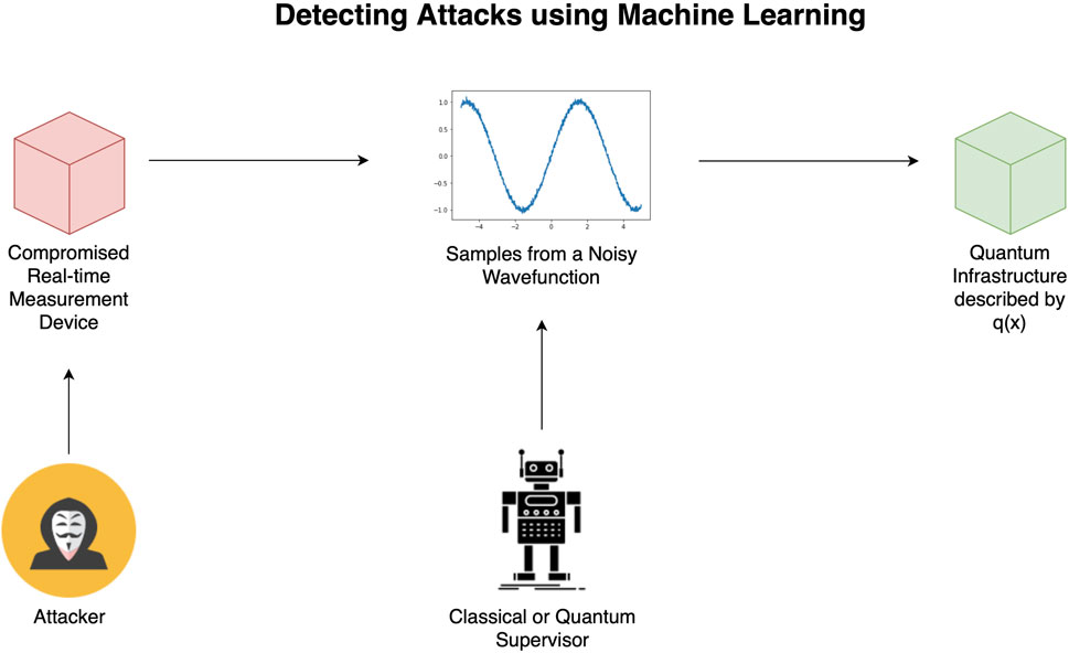
FIGURE 2. Scenario where a classical or quantum ML algorithm observes samples from the waveform and predicts whether these are regular noisy samples or anomalous samples injected by an attacker. This is done by learning the function $a(q(p)):{\mathbb{R}}^u\to \{\text{normal\hspace{0.17em},\hspace{0.17em}FDI}\}$ discussed in the scenario for Figure 1.

4 Problem formulation

We are focused on False Data Injection (FDI) attacks, as shown in the scenario of Figure 1, which involves the differentiation of legitimate noisy sampled data and anomalous, attacker-supplied FDI data in the quantum infrastructure. This is accomplished by training an ML/QML algorithm to classify real-time data into normal and FDI classes. More formally, the problem can be formulated analytically as follows:

1. We define points

$p^{\text{normal}}={\left\{p_i^{\text{normal}}\right\}}_{i=1}^n$

belonging to a class ${\mathcal{C}}_{\text{normal}}$ which represent normal, non-FDI data, and points

$p^{\text{FDI}}={\left\{p_j^{\text{FDI}}\right\}}_{j=1}^m$

belonging to a class ${\mathcal{C}}_{\text{FDI}}$ which represent FDI data. Each point p_i represents (x_i, y_i) horizontal and vertical axis values sampled from the waveform outputted by an RTMD. Usually, the sets p^normal and p^FDI would be created in a constructive way; however, in this paper, p^normal and p^FDI are created through the assignment algorithm presented in Section 5, which defines a function

$a\left(q\left(p\right)\right):{\mathbb{R}}^u\to \left\{\text{normal\hspace{0.17em},\hspace{0.17em}FDI}\right\}$

that takes in points ${\{p_k\}}_{k=1}^{n+m}$, $p_k\in {\mathbb{R}}^u$ and splits them into two sets p^normal and p^FDI.

2. We set up the assignment problem by creating a waveform f(x) and sampling points

${\left\{p_k=\left(x_k,y_k=f\left(x_k\right)\right)\right\}}_{k=1}^{n+m}$

from it to use as an input to the assignment problem. We search for an f(x) that results in an assignment problem that shows an optimal cyberattack detection separation between a QML and ML algorithm; our methodology is presented in Section 5.

3. We define a classical learning algorithm ${\mathcal{L}}^{\text{classical}}$ and a quantum learning algorithm ${\mathcal{L}}^{\text{quantum}}$ to learn the function $a(q(p)):{\mathbb{R}}^u\to \{\text{normal\hspace{0.17em},\hspace{0.17em}FDI}\}$ and we evaluate them in Section 7 through the use of the accuracy metric.

The definition of $a(q(p)):{\mathbb{R}}^u\to \{\text{normal\hspace{0.17em},\hspace{0.17em}FDI}\}$ is an entirely new contribution of this feature, and results in a previously unseen dataset so it is not straightforward to compare our experimental results to previous literature. However, this paper provides a starting foundation for comparing the many candidates for the cyberattack detection algorithms ${\mathcal{L}}^{\text{classical}}$ and ${\mathcal{L}}^{\text{quantum}}$ which have previously been proposed in the literature on the newly generated datasets p^normal and p^FDI we provide here. We leave this to future work.

5 FDI attack construction

The scenario of Figure 1 relies on differentiating between legitimate noisy samples p^normal and anomalous, attacker-injected samples p^FDI in the quantum infrastructure. When generating a corresponding supervised learning dataset, there are two questions to consider:

1. What kind of noisy waveform should be considered?

2. Suppose that the waveform is sampled. How does one decide which samples correspond to the regular noisy process and which samples correspond to a cyberattack? In other words, how is the function a(q(p)) defined in the scenario in Figure 1?

Question (1) can be momentarily deferred. Assume that the waveform is given. For example, consider the 60 Hz waveform shown in the upper left of Figure 3. Suppose that something goes wrong with the measurement process, and the wavefunction becomes noisy after x = 0.1. In addition, suppose that there are 30 randomly spaced samples ${\{p_k\}}_{k=1}^{30}$ from this noisy function (These correspond to the ${\{p_k\}}_{k=1}^{n+m}$ discussed in Section 4). This is shown in the upper right of Figure 3.

FIGURE 3

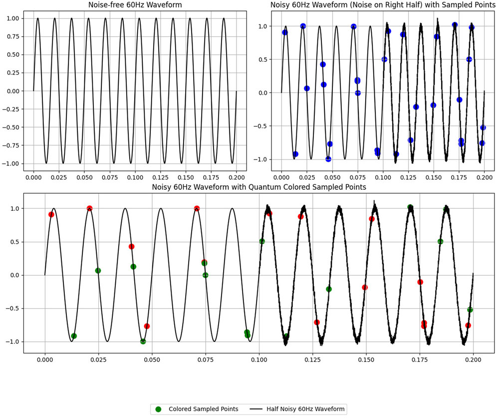
FIGURE 3. Generated waveforms: Noise-free, with half noisy region, and with quantum-colored sampled points. Green points represent samples belonging to ∖operational and red points represent samples belonging to ∖malfunction.

To keep things simple, let ${\mathcal{C}}_{\text{normal}}$ and ${\mathcal{C}}_{\text{FDI}}$ have the same number of points. The goal is to split ${\{p_k\}}_{k=1}^{30}$ into ${\{p_i^{\text{normal}}\}}_{i=1}^{15}$ and ${\{p_j^{\text{FDI}}\}}_{j=1}^{15}$ (Corresponding to p^normal and p^FDI in Section 4). This function visibly changes behaviour and becomes much more noisy at x = 0.1, so the trivial labelling would be to assign the samples which are less than or equal to 0.1 to ${\mathcal{C}}_{\text{normal}}$ and the others to ${\mathcal{C}}_{\text{FDI}}$. However, recall that we aim to explore the maximum cyberattack detection advantage of ${\mathcal{L}}^{\text{classical}}$ over ${\mathcal{L}}^{\text{quantum}}$. Our proposed trivial labelling will likely not result in an advantage; in fact, such a labelling does not require any machine learning at all and can be done by just visually examining the waveform. Moreover, the labelling approach did not include the notion of quantum infrastructure making the trivial data sets under consideration classical, not quantum.

Fortunately, there is a way to optimally solve the assignment problem to p^normal and p^FDI to maximally separate ${\mathcal{L}}^{\text{classical}}$ and ${\mathcal{L}}^{\text{classical}}$. Given ${\{x_k\}}_{k=1}^{n+m}$, the first step is to define a new dataset $\mathcal{X}\in {\mathbb{R}}^{n\times 2}$ where each row is a tuple $\left(x_k,y_k=f(x_k)\right.$. In other words, $\mathcal{X}$ is simply a dataset of samples from the graph of the function f. The next step is to use $\mathcal{X}$ as an input to a quantum algorithmic primitive proposed in the literature (Huang et al., 2021b) which makes use of the theory of classical (Müller et al., 2018) and quantum kernels (Schuld and Killoran, 2019) to automatically assign labels to a dataset in such a way as to provide a quantum predictive advantage (if one exists)¹. As mentioned in Section 2, a quantum kernel is simply a kernel that makes use of a quantum device in order to estimate a feature map, that is, difficult to compute on a classical computer. This algorithmic primitive can be thought of as depending on a theoretical quantum device and we can thus think of it as playing the role of the function a(q(p)) discussed in the scenario in Figure 3.

The primitive works as follows: suppose that $\mathcal{X}$ is the dataset described above, k^C is a classical kernel, and k^Q is a quantum kernel. Let G^C be the Gram matrix associated with $\mathcal{X}$ and k^C, and let G^Q be the Gram matrix associated with $\mathcal{X}{k}^Q$. Note that if one is given a dataset $\mathcal{X}\in {\mathbb{R}}^{n\times m}$ and a kernel function $k:{\mathbb{R}}^m\times {\mathbb{R}}^m\to \mathbb{R}$, the associated Gram matrix G is an n × n matrix with $G_{ij}=k({\mathcal{X}}^{(i)},{\mathcal{X}}^{(j)})$ with ${\mathcal{X}}^{(i)}$ and ${\mathcal{X}}^{(j)}$ respectively denoting the ith and jth rows of $\mathcal{X}$. We refer the reader to (Huang et al., 2021b) for a proof, but the continuous label vector showing the maximal quantum advantage according to the given kernels is

$l=\sqrt{G^{Q}v}(1)$

where v is the eigenvector of $M=\sqrt{G^Q}{(G^C)}^{-1}\sqrt{G^Q}$ corresponding to the eigenvalue $\parallel \sqrt{G^Q}{(G^C)}^{-1}\sqrt{G^Q}{\parallel }_{\infty }$. Note that ∥ M ∥_∞ is the Schatten ∞-norm which corresponds to the induced 2-norm, i.e., the spectral norm. This label vector is continuous: since our area of interest is binary classification problems, we can transform the label vector to our use-case by defining the binary classification labels to be $l_k^b=(l_k>\text{median}(l))$ and potentially adding some noise to make the problem more difficult. The dataset ${\{p_k,l_k^b\}}_{k=1}^{n+m}$ represents the generated supervised learning problem; the entries p^normal where l_k is equal to 0 correspond to the normal points, and the entries p^FDI where l_k is equal to 1 correspond to the FDI points.

In this paper, we generate the labels by setting the classical kernel to be the radial basis function kernel $k^C({\mathcal{X}}^{(i)},{\mathcal{X}}^{(j)})=\mathrm{e}\mathrm{x}\mathrm{p}\left\{-\gamma \parallel {\mathcal{X}}^{(i)}-{\mathcal{X}}^{(j)}{\parallel }_2^2\right\}$ and setting the quantum kernel to be a projected quantum kernel introduced in Huang et al. (2021b) and defined as $k^Q({\mathcal{X}}^{(i)},{\mathcal{X}}^{(j)})=\mathrm{e}\mathrm{x}\mathrm{p}\left\{-\gamma \parallel \rho ({\mathcal{X}}^{(i)})-\rho ({\mathcal{X}}^{(j)}){\parallel }_2^2\right\}$ with $\rho ({\mathcal{X}}^{(i)})$ being a quantum feature map. The specific quantum feature map $\rho ({\mathcal{X}}^{(i)};n_{\text{trotter}})$ that we use is the 1-reduced density matrix (Nielsen and Chuang, 2002) on all qubits of

$V{\left({\mathcal{X}}^{\left(i\right)}/n_{\text{trotter}}\right)}^{n_{\text{trotter}}}{U}_{\mathit{1qb}}|0\rangle (2)$

where |0⟩ is the computational basis state (Nielsen and Chuang, 2002), U_1qb is a wall of random qubit rotations, and $V(x)=e^{-i{\displaystyle \sum _k}{\mathcal{X}}_k^{(i)}(X_k{X}_{k+1}{Y}_k{Y}_{k+1}{Z}_k{Z}_{k+1})}$ with ${\mathcal{X}}_k^{(i)}$ indicating the kth entry of ${\mathcal{X}}^{(i)}$, and X_k, Y_k, Z_k representing the Pauli gates acting on the kth qubit. We set n_trotter = 10 and add noise by random flipping 5% of the labels when computing l_b = (l > median(l)). We chose this quantum feature map (called a Hamiltonian evolution ansatz) because it shows a large quantum advantage in Huang et al. (2021b), but other choices are also valid.

The bottom subfigure of Figure 3 shows the coloring obtained if one applies the quantum algorithmic primitive to the waveform and samples shown in the upper right of Figure 3. The coloring of a sample (x, y) can be thought of as denoting whether the associated noisy value y = f(x) + ϵ is normal at time x or whether it represents a cyberattack. Note that, to our classical eyes, these samples look effectively random but they are in fact close together in quantum space even though they are far apart in classical space. We note that if one is simulating a more realistic cyberattack detection problem, the amount of samples assigned to ${\mathcal{C}}_{\text{FDI}}$ has to be much smaller than that of the points labeled assigned to ${\mathcal{C}}_{\text{normal}}$ since anomaly detection tasks typically involve imbalanced datasets. However, as a first step and for the purposes of this paper, we keep things simple with a balanced dataset. Our future work on this topic will certainly include an imbalance and will feature a thorough study of the performance of QML when faced with imbalanced domains, along with a comparison to its classical counterpart.

It is intuitive that, depending on the shape of the waveform and the sampling rate, different amounts of quantum advantages will be obtained by QML algorithms. Inalgorithms. In this section, we have assumed that the waveform of interest was given to us and explained how an algorithm proposed in the literature can be used to generate difficult quantum labels that fit the scenario in Figure 2. This paper’s main contribution, however, comes in Section 6 where we will show how we can tackle the interesting problem of finding waveforms that show the maximal quantum advantage through the evolution of random fourier functions.

6 Evolving noisy finite fourier series

Section 5 assumes that the noisy waveform of interest is given. However, since the data is being synthetically generated, this is obviously not the case in practice and a waveform must be manually defined. Seeing as the goal behind this paper is to study regimes where a large quantum advantage is possible, a natural decision is to automatically explore waveform shapes that result in the maximum possible quantum advantage. In order to do this, the first thing, that is, needed is a parametrized function space of waveforms. One possible way to define this space is to make use of the proposed random finite Fourier series in Filip et al. (2019), where the authors define smooth random functions which are periodic on an interval [−L/2, L/2] as

$f\left(x\right)=a_0+\sqrt{2}\sum _{j=1}^m\left[a_j\cos \left(\frac{2\pi jx}{L}\right)+b_j\sin \left(\frac{2\pi jx}{L}\right)\right](3)$

where λ > 0 is a wavelength parameter and m = ⌊L/λ⌋. Let a = [a₀, a₁, …a_m] and b = [b₁, …b_m], and let ${\{x_i\}}_{i=1}^n$ be a set of user-defined points representing a discretization of the domain over which to evolve the function. A perturbation can be added in order to evolve noisy functions, so let $ϵ\in {\mathbb{R}}^u$ be vector which contains an ${ϵ}_i\in \mathbb{R}$ perturbation for all ${\{x_i\}}_{i=1}^n$. Each ϵ_i can represent either a perturbation arising from regular noise or a perturbation resulting from a cyberattack attempt. Let $\theta =[a,b,ϵ]\in {\mathbb{R}}^{2m+1+n}$ be a vector concatenation of a, b, ϵ. Then the noisy function can b be written in the following way:

$f\left(x_i;\theta \right)=a_0+\sqrt{2}\sum _{j=1}^m\left[a_j\cos \left(\frac{2\pi j{x}_i}{L}\right)+b_j\sin \left(\frac{2\pi j{x}_i}{L}\right)+{ϵ}_i\right](4)$

where the parametrization on θ has been made clear and we have renamed the function argument x to x_i to make its relationship to ϵ_i clearer. Then the space to be explored during optimization is

${\left\{f\left(x_1;\theta \right),f\left(x_2;\theta \right),\dots ,f\left(x_n;\theta \right)\right\}}_{\theta \in {\mathbb{R}}^{2m+1+n}}(5)$

One can also choose subsets of R^2m+1+n instead of the whole set. In this formulation, the goal is to explore values of θ which maximize the potential quantum advantage, and we keep λ as a user defined parameter. Letting λ be user defined instead of incorporating it as part of the optimization process has the advantage of giving the user much greater control in the type of experiment we perform since it has a drastic effect on the potential waveform shapes, thus allowing them to easily shoehorn themselves into particular regions of function space across different experiments.

This maximization problem also requires some way of quantifying potential quantum advantage, and luckily, the work in Huang et al. (2021b) provides a solution: if one is given the dataset $\mathcal{X}$, the radial basis function and projected quantum kernels k^C and k^Q described in Section 5, and uses them to compute the Gram matrices G^C and G^Q described in Section 5, the potential for quantum advantage can be represented by the following quantity:

$g\left(G^C|G^Q\right)=\sqrt{\parallel \sqrt{G^Q}{\left(G^C\right)}^{-1}\sqrt{G^Q}{\parallel }_{\infty }}(6)$

The quantity g(G^C | G^Q) is called the geometric difference between the classical and quantum kernels. Roughly speaking, g(G^C | G^Q) checks whether the dataset points that are close together in the feature space defined by the quantum kernel align well with the dataset points that are close together in the feature space defined by the classical kernel. If g(G^C | G^Q) is small, it means that there is a good alignment between the classical and quantum kernels and there is no potential advantage since the two kernels are essentially “clustering” the dataset points the same way. However, if g(G^C | G^Q) is large, then there exists the potential for a quantum advantage.

Let h(k; θ) be the function that first forms the dataset $\mathcal{X}\in {\mathbb{R}}^{n\times 2}$ by computing each row ${\mathcal{X}}^{(i)}$ as (x_i, f(x_i; θ)), and then computes the Gram matrix G corresponding to the matrix $\mathcal{X}$ and the given kernel k. Then, in order to generate a waveform whose associated dataset $\mathcal{X}$ has the potential for a quantum advantage, we need to solve the following maximization problem:

$\underset{\theta \in {\mathbb{R}}^{2m+1+n}}{\max }g\left(h\left(k^C;\theta \right)|h\left(k^Q;\theta \right)\right)(7)$

This is a fairly complicated problem, but seeing as θ is a continuous parameter, it can be solved by the popular gradient-free, black box, high performing and paralellizable differential evolution algorithm (Storn and Price, 1997). Differential evolution can be explained through one of its simple variants. We first initialize a population of N candidate solutions ${\{{\theta }^{(j)}\}}_{j=1}^N$. Each θ^(j) can be initialized by sampling the entries $a_i^{(j)}$ and $b_i^{(j)}$ from $\mathcal{N}(\mathrm{0,1}/(2m+1))$ as proposed in Filip et al. (2019), and sampling ϵ^(j) from $\mathcal{N}(\mu ,\sigma )$ for some user-defined μ and σ. Then a simple differential evolution variant iteratively refines the candidates by doing the following for each θ⁽ⁱ⁾:

1. Randomly choosing 3 candidates θ⁽¹⁾, θ⁽²⁾, and θ⁽³⁾ from the current population and computing θ′ = θ⁽¹⁾ + (θ⁽²⁾ − θ⁽³⁾)/2.

2. Randomly swapping components between θ⁽ⁱ⁾ and θ′.

3. Replacing θ⁽ⁱ⁾ by θ′ if and only if θ′ has a better fitness value.

By repeating the above for a particular number of iterations or until a desired fitness is reached, one arrives at an acceptable solution, which in our case are the parameters that define an anomalous waveform having a high potential for quantum advantage in the scenarios proposed in 3. For our purposes, we simply initialize the population as described above and use scipy’s (Virtanen et al., 2020) built-in differential evolution algorithm to maximize the geometric difference.

7 Experiments and results

As mentioned in Section 6, we use scipy’s (Virtanen et al., 2020) differential evolution algorithm to optimize the θ parameter. We consider three different experiments, each corresponding to a different value of the λ wavelength parameter, and we run the differential evolution algorithm for 6 h on a colab notebook for each of these experiments. The rest of the experimental parameters used in scipy and for the noisy finite fourier series are shown in Table 1 As mentioned.

TABLE 1

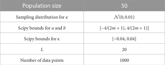
TABLE 1. Experimental parameters used. The data points are obtained by sampling 1000 equally spaced points from [−L/2, L/2]. We chose to sample 1000 points since it is a good compromise between having enough data to learn from for both classical and quantum ML algorithms, and showing the advantages of QML when learning from a small amount of quantum data, a phenomenon which is explored in Huang et al. (2021b). We chose L = 20 in order to space these 1000 points out slightly and not make them too close. As mentioned in Section 6, a and b are initially sampled from $\mathcal{N}(\mathrm{0,1}/(2m+1))$, so we simply set their scipy lower and upper bounds to be −4 and 4 times the normal distribution’s standard deviation and the same logic holds for the ϵ bounds.

The optimal wavefunctions found by the differential evolution algorithm, along with their quantum algorithmic primitive coloring, are presented in Figure 4; Figure 5; Figure 6. We observe that although the coloring appears random, the red and green points are, in fact, separated into two distinguishable clusters in quantum feature space. The shape of these wavefunctions provide us a sense of how future waveforms need to be structured to exhibit maximal quantum advantage within the scenario described in Figure 1. We then compare the performance of classical machine learning vs. QML in predicting the labels of the sampled points (green vs. red). We define the classical algorithm to be a neural network that takes in normal features which consist of (x, y) samples from the graph, and we define the quantum algorithm to be a neural network with the same architecture that takes in the quantum features that correspond to the 1-reduced density matrix discussed in Section 5. This approach is meant to optimize the QML advantage while still providing a somewhat compatible and fair comparison from the perspective that the hidden architectures are similar. We scaled both sets separately to have a mean of zero and a unit standard deviation to facilitate the optimization process. We choose a fully connected architecture of (128, 64, 32, 16) hidden ReLU neurons followed by a single sigmoidal neuron.

FIGURE 4

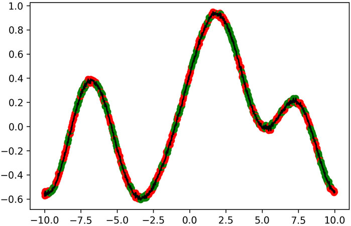
FIGURE 4. Wavefunction evolved in the experiment corresponding to λ =5, colored according to the labels found by the quantum algorithmic primitive discussed in Section 5. The function is plotted within its periodic interval of [−L/2, L/2].

FIGURE 5

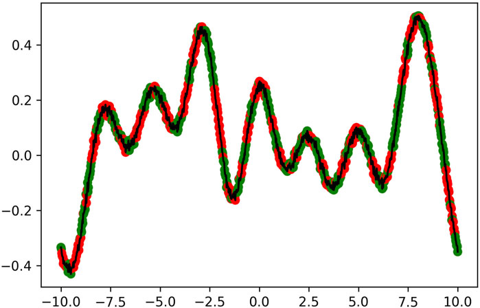
FIGURE 5. Wavefunction evolved in the experiment corresponding to λ = 2.5, colored according to the labels found by the quantum algorithmic primitive discussed in Section 5. The function is plotted within its periodic interval of [−L/2, L/2].

FIGURE 6

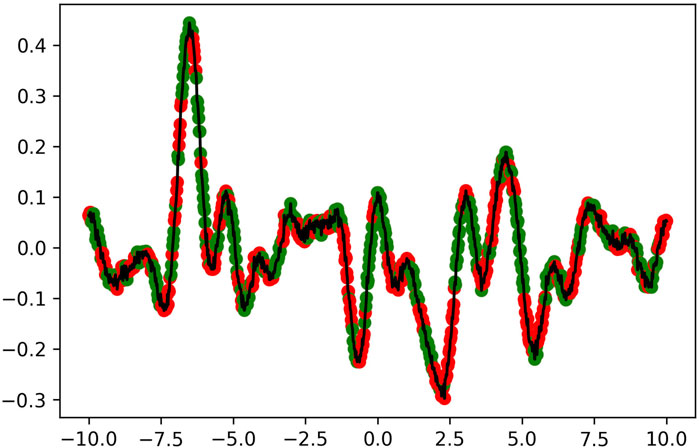
FIGURE 6. Wavefunction evolved in the experiment corresponding to λ = 1, colored according to the labels found by the quantum algorithmic primitive discussed in Section 5. The function is plotted within its periodic interval of [−L/2, L/2].

The networks were trained with a binary cross-entropy loss for 500 epochs using the ADAM optimizer, and the 10-fold cross validation results are shown in Table 2; Table 3; Table 4. The difference in performance grows as the wavelength decreases, starting from an approximately 7 percentage points difference in accuracy for λ = 5, and growing to a more than 25 percentage points difference for λ = 1. In addition, note that the performance of the QML algorithm stays relatively stable across all wavelengths, and it is only the classical performance that decreases. These results indicate that wavefunctions with shorter wavelengths have more potential for a quantum advantage in the RTMD scenario considered in this paper. Whether an analogous version of this result holds for higher dimensional waveforms remains to be seen and is an interesting topic for a future line of work. The results in this section indicate a stunning potential difference in performance between QML and classical ML when it comes to quantum data, and this is the kind of advantage that must be achieved in order to make QML practical.

TABLE 2

TABLE 2. 10-fold cross validation results for the classical and quantum ML algorithms for the first experiment (λ = 5). The result reported is of the form ($\bar{s}$; STD; MAD) where $\bar{s}\in \{\text{accuracy,\hspace{0.17em}precision\hspace{0.17em},\hspace{0.17em}recall\hspace{0.17em},\hspace{0.17em}F}1\text{\hspace{0.17em}score}\}$ is the mean metric across the 10 folds and STD and MAD respectively denote the standard deviation and median absolute deviation.

TABLE 3

TABLE 3. 10-fold cross validation results for the classical and quantum ML algorithms for the second experiment (λ = 2.5). The result reported is of the same form as in Table 2.

TABLE 4

TABLE 4. 10-fold cross validation results for the classical and quantum ML algorithms for the third experiment (λ = 1). The result reported is of the same form as in Table 2.

8 Conclusion and future work

In this paper, we have introduced some fundamental scenarios regarding how quantum data may arise in a future smart grid. We have explored quantum learning in one of these scenarios by combining a previously proposed quantum algorithmic primitive that generates classically-difficult synthetic labels with an original differential evolution algorithm to optimize over a space of noisy wavefunctions. Our results demonstrate that wavefunctions with a smaller wavelength are more likely to exhibit a quantum advantage, with this advantage reaching a difference of more than 25 accuracy percentage points in favor of the quantum learner. This implies that these types of wavefunctions are a more promising potential avenue for a quantum advantage in smart grid scenarios that resemble the one explored in this paper. To the best of our knowledge, this is the first work that conducts empirical studies on QML for quantum data in smart grids.

There are many possible lines of avenues for future work. The first and most obvious is to explore the remaining scenarios presented in this paper. The second is to extend the ideas and experiments to other settings such as multivariate waveforms. The third, and possibly most important line of work, is to generate synthetic labels by making use of quantum circuit architectures that are more relevant to the smart grid than the Hamiltonian evolution architecture used here.

We emphasize that given quantum technologies are still in their infancy, our goal in writing this paper was not to propose a quantum algorithm for current deployment, but was rather to propose ways to effectively nudge QML for smart grids towards quantum data scenarios. We argue that this is more promising than classical data scenarios because of the overhead imposed by quantum error correction. We believe that the potential exponential advantages offered by a successful transition will prove worthwhile in the years to come.

Data availability statement

Due to confidentiality requirements established with the industry funding partner, data is not publicly available for this paper. Special requests to access the datasets should be directed to andrew.nader@mail.utoronto.ca.

Author contributions

The ideas and research in this paper were initiated and developed by AN with feedback from M-AD and under the supervisor of DK. All authors contributed to the article and approved the submitted version.

Funding

Funding is gratefully acknowledged by Mitacs and Hydro-Québec under the Mitacs Accelerate Cluster program.

Conflict of interest

The authors declare that the research was conducted in the absence of any commercial or financial relationships that could be construed as a potential conflict of interest.

Publisher’s note

All claims expressed in this article are solely those of the authors and do not necessarily represent those of their affiliated organizations, or those of the publisher, the editors and the reviewers. Any product that may be evaluated in this article, or claim that may be made by its manufacturer, is not guaranteed or endorsed by the publisher.

Footnotes

¹Note that the work in Huang et al. (2021b) does not mention smart grids or waveforms, but rather deals with general quantum dataset creation given an arbitrary matrix $\mathcal{X}\in {\mathbb{R}}^{n\times m}$.

References

Aaronson, S. (2004). Is quantum mechanics an island in theoryspace? arXiv preprint quant-ph/0401062.

Google Scholar

Albash, T., and Lidar, D. A. (2018). Adiabatic quantum computation. Rev. Mod. Phys. 90, 015002. doi:10.1103/revmodphys.90.015002

CrossRef Full Text | Google Scholar

Ashrafuzzaman, M., Das, S., Chakhchoukh, Y., Shiva, S., and Sheldon, F. T. (2020). Detecting stealthy false data injection attacks in the smart grid using ensemble-based machine learning. Comput. Secur. 97, 101994. doi:10.1016/j.cose.2020.101994

CrossRef Full Text | Google Scholar

Babbush, R., McClean, J. R., Newman, M., Gidney, C., Boixo, S., and Neven, H. (2021). Focus beyond quadratic speedups for error-corrected quantum advantage. PRX Quantum 2, 010103. doi:10.1103/prxquantum.2.010103

CrossRef Full Text | Google Scholar

Benedetti, M., Lloyd, E., Sack, S., and Fiorentini, M. (2019). Parameterized quantum circuits as machine learning models. Quantum Sci. Technol. 4, 043001. doi:10.1088/2058-9565/ab4eb5

CrossRef Full Text | Google Scholar

Brown, K. L., Munro, W. J., and Kendon, V. M. (2010). Using quantum computers for quantum simulation. Entropy 12, 2268–2307. doi:10.3390/e12112268

CrossRef Full Text | Google Scholar

Chia, N.-H., Gilyén, A., Li, T., Lin, H.-H., Tang, E., and Wang, C. (2020). “Sampling-based sublinear low-rank matrix arithmetic framework for dequantizing quantum machine learning,” in Proceedings of the 52nd Annual ACM SIGACT symposium on theory of computing, 387–400.

CrossRef Full Text | Google Scholar

Crawford, S. E., Shugayev, R. A., Paudel, H. P., Lu, P., Syamlal, M., Ohodnicki, P. R., et al. (2021). Quantum sensing for energy applications: review and perspective. Adv. Quantum Technol. 4, 2100049. doi:10.1002/qute.202100049

CrossRef Full Text | Google Scholar

Creswell, A., White, T., Dumoulin, V., Arulkumaran, K., Sengupta, B., and Bharath, A. A. (2018). Generative adversarial networks: an overview. IEEE signal Process. Mag. 35, 53–65. doi:10.1109/msp.2017.2765202

CrossRef Full Text | Google Scholar

Crosson, E., and Lidar, D. (2021). Prospects for quantum enhancement with diabatic quantum annealing. Nat. Rev. Phys. 3, 466–489. doi:10.1038/s42254-021-00313-6

CrossRef Full Text | Google Scholar

Degen, C. L., Reinhard, F., and Cappellaro, P. (2017). Quantum sensing. Rev. Mod. Phys. 89, 035002. doi:10.1103/revmodphys.89.035002

CrossRef Full Text | Google Scholar

Filip, S., Javeed, A., and Trefethen, L. N. (2019). Smooth random functions, random odes, and Gaussian processes. SIAM Rev. 61, 185–205. doi:10.1137/17m1161853

CrossRef Full Text | Google Scholar

Gisin, N., Ribordy, G., Tittel, W., and Zbinden, H. (2002). Quantum cryptography. Rev. Mod. Phys. 74, 145–195. doi:10.1103/revmodphys.74.145

CrossRef Full Text | Google Scholar

Harrow, A. W., Hassidim, A., and Lloyd, S. (2009). Quantum algorithm for linear systems of equations. Phys. Rev. Lett. 103, 150502. doi:10.1103/physrevlett.103.150502

PubMed Abstract | CrossRef Full Text | Google Scholar

Harrow, A. W. (2020). Small quantum computers and large classical data sets. arXiv preprint arXiv:2004.00026.

Google Scholar

Huang, H.-Y., Broughton, M., Cotler, J., Chen, S., Li, J., Mohseni, M., et al. (2021a). Quantum advantage in learning from experiments. arXiv preprint arXiv:2112.00778.

Google Scholar

Huang, H.-Y., Broughton, M., Mohseni, M., Babbush, R., Boixo, S., Neven, H., et al. (2021b). Power of data in quantum machine learning. Nat. Commun. 12, 2631. doi:10.1038/s41467-021-22539-9

PubMed Abstract | CrossRef Full Text | Google Scholar

Irfan, M., Sadighian, A., Tanveer, A., Al-Naimi, S. J., and Oligeri, G. (2023). False data injection attacks in smart grids: State of the art and way forward. arXiv preprint arXiv:2308.10268.

Google Scholar

Jahromi, M. Z., Jahromi, A. A., Kundur, D., Sanner, S., and Kassouf, M. (2021). Data analytics for cybersecurity enhancement of transformer protection. ACM SIGENERGY Energy Inf. Rev. 1, 12–19. doi:10.1145/3508467.3508469

CrossRef Full Text | Google Scholar

Jahromi, M. Z., Jahromi, A. A., Sanner, S., Kundur, D., and Kassouf, M. (2020). “Cybersecurity enhancement of transformer differential protection using machine learning,” in IEEE Power & Energy Society General Meeting (PESGM) (IEEE), 1–5.

CrossRef Full Text | Google Scholar

Karimipour, H., Dehghantanha, A., Parizi, R. M., Choo, K.-K. R., and Leung, H. (2019). A deep and scalable unsupervised machine learning system for cyber-attack detection in large-scale smart grids. IEEE Access 7, 80778–80788. doi:10.1109/access.2019.2920326

CrossRef Full Text | Google Scholar

Kerenidis, I., and Prakash, A. (2016). Quantum recommendation systems. arXiv preprint arXiv:1603.08675.

Google Scholar

Khaw, Y. M., Jahromi, A. A., Arani, M. F., Sanner, S., Kundur, D., and Kassouf, M. (2020). A deep learning-based cyberattack detection system for transmission protective relays. IEEE Trans. Smart Grid 12, 2554–2565. doi:10.1109/tsg.2020.3040361

CrossRef Full Text | Google Scholar

Lloyd, S., Mohseni, M., and Rebentrost, P. (2013). Quantum algorithms for supervised and unsupervised machine learning. arXiv preprint arXiv:1307.0411.

Google Scholar

Lukens, J. M., Passian, A., Yoginath, S., Law, K. J., and Dawson, J. A. (2022). Bayesian estimation of oscillator parameters: toward anomaly detection and cyber-physical system security. Sensors 22, 6112. doi:10.3390/s22166112

PubMed Abstract | CrossRef Full Text | Google Scholar

Luo, Y., Cai, X., Zhang, Y., Xu, J., and Yuan, X. (2018). Multivariate time series imputation with generative adversarial networks. Adv. neural Inf. Process. Syst. 31.

Google Scholar

Müller, K.-R., Mika, S., Tsuda, K., and Schölkopf, K. (2018). Handbook of neural network signal processing. CRC Press, 4–1.An introduction to kernel-based learning algorithms

Google Scholar

Nielsen, M. A., and Chuang, I. (2002). Quantum computation and quantum information.

Google Scholar

Niu, S., Liu, Y., Wang, J., and Song, H. (2020). A decade survey of transfer learning (2010–2020). IEEE Trans. Artif. Intell. 1, 151–166. doi:10.1109/tai.2021.3054609

CrossRef Full Text | Google Scholar

Pirandola, S., Andersen, U. L., Banchi, L., Berta, M., Bunandar, D., Colbeck, R., et al. (2020). Advances in quantum cryptography. Adv. Opt. photonics 12, 1012–1236. doi:10.1364/aop.361502

CrossRef Full Text | Google Scholar

Schuld, M., and Killoran, N. (2019). Quantum machine learning in feature hilbert spaces. Phys. Rev. Lett. 122, 040504. doi:10.1103/physrevlett.122.040504

PubMed Abstract | CrossRef Full Text | Google Scholar

Shor, P. W. (1999). Polynomial-time algorithms for prime factorization and discrete logarithms on a quantum computer. SIAM Rev. 41, 303–332. doi:10.1137/s0036144598347011

CrossRef Full Text | Google Scholar

Storn, R., and Price, K. (1997). Differential evolution–a simple and efficient heuristic for global optimization over continuous spaces. J. Glob. Optim. 11, 341–359. doi:10.1023/a:1008202821328

CrossRef Full Text | Google Scholar

Tang, E. (2019). “A quantum-inspired classical algorithm for recommendation systems,” in Proceedings of the 51st Annual ACM SIGACT Symposium on Theory of Computing, 217–228.

CrossRef Full Text | Google Scholar

Tang, E. (2021). Quantum principal component analysis only achieves an exponential speedup because of its state preparation assumptions. Phys. Rev. Lett. 127, 060503. doi:10.1103/physrevlett.127.060503

PubMed Abstract | CrossRef Full Text | Google Scholar

Ullah, M. H., Eskandarpour, R., Zheng, H., and Khodaei, A. (2022). IET generation. Transmission & Distribution.Quantum computing for smart grid applications

CrossRef Full Text | Google Scholar

Virtanen, P., Gommers, R., Oliphant, T. E., Haberland, M., Reddy, T., Cournapeau, D., et al. (2020). SciPy 1.0: fundamental algorithms for scientific computing in Python. Nat. Methods 17, 261–272. doi:10.1038/s41592-019-0686-2

PubMed Abstract | CrossRef Full Text | Google Scholar

Zhang, J. E., Wu, D., and Boulet, B. (2021). “Time series anomaly detection for smart grids: A survey,” in 2021 IEEE Electrical Power and Energy Conference (EPEC) (IEEE), 125–130.

CrossRef Full Text | Google Scholar

Zhang, J., Zhang, X., Yang, J., Wang, Z., Zhang, Y., Ai, Q., et al. (2020). “Deep lstm and gan based short-term load forecasting method at the zone level,” in 2020 International Conference on Artificial Intelligence in Information and Communication (ICAIIC) (IEEE), 613–618.

CrossRef Full Text | Google Scholar

Zhou, Y., and Zhang, P. (2021). Quantum machine learning for power system stability assessment.

Google Scholar