Study on Obtaining Real Power Curve of Wind Turbines Using SCADA Data

The key problem to be solved in the process of wind turbine (WT) operation and maintenance is to obtain the wind turbine performance accurately. The power curve is an important indicator to evaluate the performance of wind turbines. How to model and obtain the power curve of wind turbines has always been one of the hot topics in research. This paper proposes a novel idea to get the actual power curve of wind turbines. Firstly, the basic data preprocessing algorithm is designed to process the zero value and null value in the original supervisory control and data acquisition (SCADA) data. The moving average filtering (MAF) method is employed to deal with the wind speed, the purpose of which is to consider the comprehensive result of wind on the wind turbine power in a certain period. According to the momentum theory of the ideal wind turbine and combined with the characteristics of the anemometer installation position, the deviation between the measured wind speed and the actual wind speed is approximately corrected. Here, the influence of dynamic changes in air density is also considered. Then, the Gaussian fitting algorithm is used to fit the wind-power curve. The characteristics of the power curve before and after wind speed correction are compared and analyzed. At the same time, the influence of the parameter uncertainty on the reliability of the power curve is considered and investigated. Finally, the characteristics of the power curves of four wind turbines are compared and analyzed. The research results show that among these power curves, WT3 and WT4 are the closest, WT2 is the next, and WT1 has the farthest deviation from the others. The research work provides a valuable basis for on-site performance evaluation, overhaul, and maintenance of wind turbines.

Introduction

The serious impact of environmental degradation has increased global interest in wind energy. In recent years, the wind power industry has developed rapidly (Dai et al., 2018a; Dawn et al., 2019). According to the wind power statistics revealed by the World Wind Energy Association (WWEA), the worldwide wind capacity has reached 744 gigawatts. In 2020, 93 gigawatts of new wind turbines were added, setting a new record. With batches of wind turbines in service, their operating efficiency (usually referred to as “power coefficient”) has become the focus because this is directly related to the economic benefits of wind farm operation (Dai et al., 2016a; Dhunny et al., 2020; Sun et al., 2020; Bakir et al., 2021). However, due to the influence of many factors, the actual power characteristic of wind turbines operating in wind farms is often inconsistent with the designed power characteristic. So, modeling and obtaining the power curve of wind turbines has always been one of the hot topics in research (Rogers et al., 2020).

The power curve of wind turbines indicates the generated power versus wind speed (Ciulla et al., 2019). It is widely used for monitoring and evaluating wind turbine performance (Pandit et al., 2020; Astolfi et al., 2021a). The abundant SCADA data of wind farms provide a good database for wind power curve research. The different techniques used for wind turbine power curve (WTPC) modeling can be divided into parametric techniques and non-parametric techniques (Lydia et al., 2014). The power generation of wind turbines will vary with external environmental conditions. To investigate the influence of external conditions on wind speed and wind turbine power, Kim et al. analyze three atmospheric factors: atmospheric stability, turbulence intensity (TI), and wind shear (Kim et al., 2021). Various factors such as the age of the wind turbine, installation location, air density, and wind direction will cause inhomogeneity among the observation data, which usually affects the accuracy of the fitted power curve. To overcome this problem, the hybrid estimation method by Mehrjoo et al. is presented, which is based on weighted balanced loss functions (Mehrjoo et al., 2021). Saint-Drenan et al. develop an open-source model that can generate the power curve of any turbine to suit the specific conditions of any site (Saint-Drenan et al., 2020). Marčiukaitis et al. present a nonlinear regression model (three-parameter exponential model) for modeling power curve with application to the wind turbine of Seirijai wind farm (in Lithuania) (Marčiukaitis et al., 2017). To get highly accurate non-parametric power curve models, Karamichailidou et al. employ artificial neural network (ANN) belonging to the radial basis function architecture and train it using non-symmetric fuzzy means (NSFM) (Karamichailidou et al., 2021). Virgolino et al. introduce a semi-parametric method that combines Gaussian process (GP) regression, standard logistic functions (SLF), and probabilistic kernel-based machine learning models (Virgolino et al., 2020). Manobel et al. present a method based on GP data pre-filtering and ANN modeling of the power curve, where the prior filtering by GP modeling can improve the network performance (Manobel et al., 2018). Mehrjoo et al. propose two non-parametric techniques, which are based on the tilt method and the monotonic spline regression, to construct the WTPC that maintains monotonicity (Mehrjoo et al., 2020). Seo et al. construct a nonlinear parametric power curve model using the logistic function, and four parameters in the logistic function are obtained explicitly by the maximum likelihood estimation (MLE) method (Seo et al., 2019). The results provided by the logistic functions are useful due to the continuity and adaptability. However, there are many types of logic functions, and how to choose is a question worth studying. From this scenario, the well-known logistic functions are employed and tested for modeling WTPC by Villanueva et al. (Villanueva and Feijóo, 2018). Yesilbudak et al. present a robust hybrid method for the power curve modeling of wind turbines, where Mahalanobis distance measure and the chi-square cumulative distribution are used for the power curve filtering (Yesilbudak, 2018). Usually, the SCADA-collected data are those averaged (typically with an averaging time of 10 min). Gonzalez et al. investigate the use of high-frequency SCADA data for wind turbine performance monitoring and propose a new framework based on multivariate non-parametric models (Gonzalez et al., 2017; Gonzalez et al., 2019).

However, the previous research mainly focused on the power curve algorithm itself, that is, how to improve the algorithm to improve the accuracy and reliability further, and the analysis of the impact caused by the physical properties of the data itself is insufficient. The knowledge gaps that need to be supplemented are mainly manifested in the following aspects, which are also the main contributions of this article.

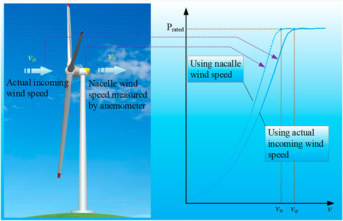
• How to obtain the data needed for reliable power curve modeling from SCADA data. In SCADA data, the wind speed is provided by the anemometer installed on the nacelle, which is not the actual incoming wind speed (Dai et al., 2016b; Dai et al., 2019). Because the wind is blowing first on the wind rotor and then on the anemometer, some of the wind energy has already been absorbed by the wind rotor, the wind speed measured by the anemometer is smaller than the actual incoming wind speed. If the wind speed data in SCADA is used directly to obtain the power curve, the deviation must be significant (Figure 1). So, different from previous studies, this article first corrects the wind speed in SCADA and then performs power curve modeling.

• How to obtain the real mapping characteristics between wind speed and power. The wind speed recorded in the SCADA data is the instantaneous wind speed (once a second). Due to the inertia of the wind turbine, the output power cannot respond to the fast wind speed but is the result of a comprehensive response to the wind speed for a period. In other words, violent fluctuation in wind speed is common. However, the violent fluctuation of wind speed does not cause the violent fluctuation of generator power in a short period. The primary reason is that the wind rotor is a large inertial system. Therefore, the key question is how to find the true mapping relationship between the two. For this purpose, the moving average filtering (MAF) method will be employed to deal with the wind speed in the following sections. Then, a reasonable filter window that meets the characteristics of wind speed and power mapping will be further found.

• How to identify the reliability of the modeled power curve. Power curve modeling involves the processing of some parameters. If there is uncertainty (deviation) in the parameter value, it will affect the accuracy of power curve modeling. For example, the air temperature is used for the power curve modeling, which is recorded in the SCADA system. However, for mountain wind farms, significant differences in distance and altitude can cause temperature data bias. In another scenario, the effect of the sensor’s error should also be considered. Specifically, the two direct parameters for power curve modeling are wind speed and power, both in the SCADA system. The reliability of wind speed data and power data in the SCADA system should be judged. In this way, the actual power curve can be obtained better.

FIGURE 1

FIGURE 1. Wind turbine and its power curve.

Wind and Power From Raw SCADA Data

In the SCADA system of the investigated wind turbines, many operation parameters, such as wind speed, the rotational speed of the wind rotor, generator side power of the converter, and grid side power of the converter, are recorded. The investigated wind turbines are 2 MW direct-driven type. For this type of wind turbines, the generator side power of the converter is the output power of the generator. If the loss of mechanical energy into electrical energy is ignored, the power output of the generator can also be approximately regarded as the mechanical energy output of the wind rotor. Therefore, the scatterplot between wind speed and generator power can be obtained by using wind speed data and generator power data, which is shown in Figures 2A–C. Here, about 57 h of SCADA data are used. Although the sampling interval is 1 s, a point is extracted every 10 s to reduce the size of the scatterplots. It should be pointed out that the wind speed data is measured by the anemometer mounted on the top of the nacelle. This means that the wind is blowing first on the wind rotor and then on the anemometer. As a result, the wind speed measured by the anemometer is smaller than the actual incoming wind speed because some of the wind energy has already been absorbed by the wind rotor. In addition, yaw misalignment tends to degrade wind turbine power production (Gao and Hong, 2021). Here, these SCADA data can be divided into three types according to the magnitude of the yaw angle: less than 5°, more than 5° but less than 10°, and more than 10°.

FIGURE 2

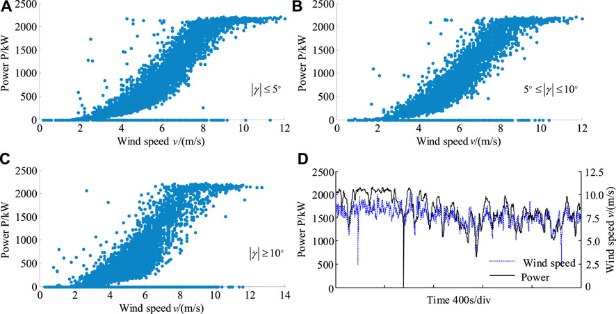
FIGURE 2. Wind and power from raw SCADA data. (A) Wind speed /(m/s). (B) Wind speed /(m/s). (C) Wind speed /(m/s). (D) Time 400s/div.

In Figure 2A, the corresponding yaw angle $\gamma$ is less than 5° and there are 7,074 sets of data. In Figure 2B, the corresponding yaw angle $\gamma$ is more than 5° but less than 10°, and there are 5,832 sets of data. In Figure 2C, the corresponding yaw angle $\gamma$ is more than 10°, and there are 7,649 sets of data. By looking at the SCADA data, it can be found that the yaw angle is scattered in different angle ranges. This is determined by the various characteristics of natural wind direction and the yaw control strategy of the wind turbine. It also means that this distribution may be different in different periods or different wind turbines, with certain randomness. It is also not difficult to find that the variation of yaw angle may affect the wind-power characteristics by comparing the distribution characteristic of the scatterplots in the three subfigures. In addition, the distribution of some points is far away from their concentrated distribution area. For example, in Figure 2A, near a wind speed of 4 m/s, there are scattered points with a power of more than 2000 kW. This is not the normal performance of a wind turbine. There are two possible reasons for this phenomenon: there may be interference signals during data collecting, and the other is that there may be instantaneous fluctuations in wind speed. Violent fluctuation in wind speed is common. However, the violent fluctuation of wind speed does not cause the violent fluctuation of generator power. The primary reason is that the wind energy is absorbed by the wind rotor, a large inertial system. In other words, the instantaneous fluctuation of the wind does not cause the instantaneous fluctuation of the rotational speed of the wind rotor. Figure 2D shows the time history curves of wind speed and generator power over a period. The data sampling interval used here is 1 s. It can be seen from this subfigure that the change frequency of wind speed is greater than the change frequency of generator power. The changing trend of wind speed and the changing trend of generator power are not identical. Due to the inherent property of wind rotor inertia, it can be considered that the influence of wind speed on generator power has a certain lag effect, and the influence of wind speed on generator power is the result of the comprehensive impact of wind in a period. Under the condition of continuous wind speed, the generator power occasionally appears zero values, which is an error in the collection process and should be eliminated. Another thing to note is that both the wind speed and the generator power are measured by sensors; thus, the reliability of the data should be confirmed. In other words, the system error of the sensor should be eliminated as far as possible. The reason for proposing this issue is that the sensors may not be calibrated regularly. For example, an anemometer may not be calibrated during several years of operation.

Overall, the following points should be attentional for the investigation of the power curve of wind turbines.

• Compensation for the deviation between the wind speed measured by the anemometer and the actual incoming wind speed should be considered.

• The effect of wind direction (yaw angle) change on actual power performance should be considered.

• The lag effect between wind speed change and generator power change should be considered.

• The error data in the data collection process should be eliminated.

• The effect of wind speed on generator power should be regarded as the comprehensive result of wind in a certain period.

• The system error of the sensors related to wind and generator power should be eliminated.

Wind Speed Data Correction

Since the effect of wind speed on generator power is the comprehensive result of wind in a certain period, it is more reasonable to model the power curve using the average of the wind speed rather than its instantaneous value. At the same time, the lag effect between wind speed variation and generator power variation is also considered. Based on these considerations, the moving average filtering (MAF) method is employed to deal with the wind speed. This method sequentially stores the data of n sampling points as a queue. When new data is collected, the first data in the queue is discarded and the arithmetic mean of the data is calculated. The discrete expression of the filter can be written as

$y\left(n\right)=\frac{1}{N+1}{\displaystyle \sum _{k=0}^{N}x\left(n-k\right)}(1)$

where, y(n) is the output of the filter, x(n) is the input of the filter, and N is the window length of the MAF filter.

Another thing to note is that null values and zero values may occur during the sensor test. If a null value appears, it is filled with zero. If a zero value appears between two normally collected data, it can be repaired by averaging the two adjacent data shown as Eq. 2. Also, this processing should be done before filtering. If multiple zeros occur consecutively, the data should be rejected.

$\{\begin{array}{l}x\left(n\right)=\text{0},\text{if}x\left(n\right)\text{is null}\\ x\left(n\right)=\frac{x\left(n-1\right)+x\left(n+1\right)}{2},\text{if }x\left(n\right)=\text{0},x\left(n-1\right)>0\text{\&}x\left(n+1\right)>0\\ x\left(n\right)=\text{0},\text{if }x\left(n+1\right)=0,x\left(n+2\right)=0,\cdot \cdot \cdot \end{array}(2)$

When using MAF filters, the critical problem is to determine the window length of the filter. Here, the basic idea to find the appropriate filter window length is to compare wind speed change trends and power change trends. Therefore, the filtered wind speed curve and the time-history power curve are given as shown in Figure 3.

FIGURE 3

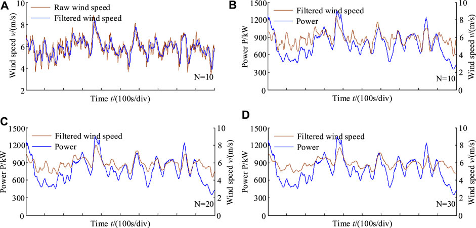
FIGURE 3. Power and the filtered wind speed. (A) Time t/(100s/div). (B) Time t/(100s/div). (C) Time t/(100s/div). (D) Time t/(100s/div).

In Figure 3A, the raw wind speed and the filtered wind speed are presented in a period. The window length N is set to be 10. The wind speed fluctuation is reduced after filtering. At the same time, the filtered wind speed curve has a slight time delay compared with the raw wind speed curve. Figures 3B–D show the wind speed curves for different filter window lengths and the corresponding time-history power curves. The longer the filter window is, the smoother the filtered wind speed curve is. Judging from the consistency of wind speed trend and power trend, it is not that the longer the filter window, the better. In contrast, a filter with a window length of 10 is better. Moreover, it should be noted that the value of the filter window length is only an approximate value because of the complexity of wind conditions.

On the other hand, the wind speed measured by the anemometer mounted on the top of the nacelle is not the actual wind speed. How to correct the wind speed has been an issue of great concern. For example, Malgaroli et al. propose a nacelle wind speed correction for evaluating wind turbine performance by estimating the wind speed entering the wind rotor (Astolfi et al., 2021b; Carullo et al., 2021). In this paper, the nacelle wind speed compensation is mainly based on the aerodynamic and energy flow characteristics of the wind turbines (Dai et al., 2016b). It should be noted here that the anemometers installed on the nacelle are considered in a normal working state. In particular, the anemometers are generally no longer calibrated regularly after service. Two issues require special consideration in the future. One is the deviation caused by the aging of the sensor itself, and the other is the deviation caused by the sensor failure.

According to the momentum theory, the power of a wind turbine to capture wind energy can be expressed as

$P=\frac{1}{2}\rho S{v}_d\left({\mathit{v}}_1^2-{\mathit{v}}_2^2\right)(3)$

where, v₁ is the upstream wind speed of the wind rotor; v_d is the wind speed passing through the wind rotor; v₂ is the downstream wind speed of the wind rotor; $\rho$ is the density of air; S is the area swept by the wind rotor.

The relationship between v₁, v_d, and v₂ can be written as (Hansen, 2008; Dai et al., 2016b)

${\mathit{v}}_2=2v_d-{\mathit{v}}_1(4)$

Substituting Eq. 4 into Eq. 3, there are

$P=2\rho S{v}_d^2\left({\mathit{v}}_1-v_d\right)(5)$

Subsequently, Eq. 5 can be transformed into (Dai et al., 2016b)

${\mathit{v}}_1=\frac{P}{2\rho S{v}_d^2}+v_d(6)$

Since the anemometer is installed near the wind rotor, the wind speed measured by the anemometer can be considered as the speed flowing through the wind rotor, that is, v_d. From Eq. 6, the deviation between the measured wind speed and the actual incoming wind speed is $P/2\rho S{v}_d^2$. Using Eq. 6, the wind speed can be further corrected.

In Eq. 6, air density $\rho$ is not a constant value, will change with ambient temperature, air pressure, and relative humidity. Furthermore, as the altitude changes, so does the atmospheric pressure. Here, the air density is calculated using the method shown in the “omni calculator” (https://www.omnicalculator.com). The calculation expression from the website is

$\{\begin{array}{l}\rho =\frac{{\text{P}}_0{e}^{\frac{-gM\left(h-h_{\text{0}}\right)}{R\cdot T_{\text{k}}}}-{\text{ P}}_{\text{V}}}{R_{\text{d}}\cdot T_{\text{K}}}+\frac{{\text{P}}_{\text{V}}}{R_{\text{v}}\cdot T_K}\\ {\text{P}}_{\text{V}}=6.1078\times {10}^{\frac{7.5T_C}{T_C+237.3}}\cdot \text{RH}\end{array}(7)$

where, $T_C$ is the measured temperature (degrees Celsius); $T_K$ is the air temperature (Kelvins); $\text{RH}$ is the relative humidity; ${\text{P}}_{\text{V}}$ is the water vapor pressure (Pa); R_d is the gas constant for dry air (287.058 J/(kg·K)); R_v is the gas constant for water vapor (461.495 J/(kg·K)); P₀ is the pressure at the sea level; g is the gravitational acceleration; M is the molar mass of air (M = 0.0289,644 kg/mol); h is the altitude; R is the universal gas constant (R = 8.31432 N m/(mol·K)).

According to the above calculation method, the corrected wind speed can be calculated, that is, the wind speed filtering is carried out according to Eq. 1, and then the wind speed deviation is corrected according to Eq. 6. In Figures 4A–D, four wind speed correction curves under different wind speed conditions are given. Overall, the corrected wind speed curves have a delay in time, smoother curves, and an increase in numerical value compared with the raw wind speed curves.

FIGURE 4

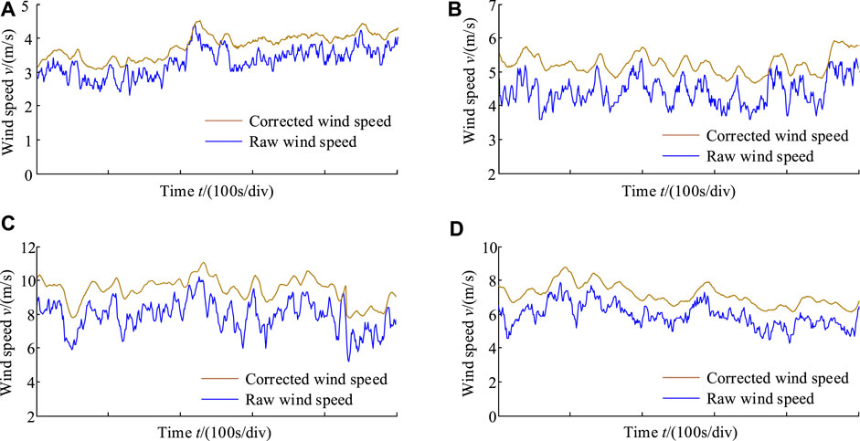
FIGURE 4. Corrected wind speed and raw wind speed. (A) Time t/(100s/div). (B) Time t/(100s/div). (C) Time t/(100s/div). (D) Time t/(100s/div).

Power Curve Model

According to the wind power theory, the power of a wind turbine is related to the inflow wind speed, rotational speed of the wind rotor, pitch angle, yaw angle, and so on. Usually, when the wind turbine is studied, the power is written as a function of wind speed and power coefficient as shown in Eq. 8. Wind speed, wind direction, the rotational speed of the wind rotor, pitch angle and air density are all variables during wind turbine operation (Dai et al., 2018b).

$P=\frac{1}{2}\rho \pi R^2{C}_{\text{P}}\left(v,\omega ,\beta ,\gamma \right)v^3(8)$

where, R is the radius of the wind rotor; $C_{\text{P}}$ is the power coefficient; $\omega$ is the rotational speed of the wind rotor; $\beta$ is the pitch angle; $\gamma$ is the yaw angle.

When a wind turbine is in regular operation, the structure parameters and control parameters have been set. The performance of the wind turbine is mainly the ability to capture wind energy, which is reflected in the relationship between power and wind speed. In other words, from the user’s point of view, the relationship between power and wind speed is their concern, which is also an important index for the on-site assessment of wind turbines. From this scenario, it is rather vital to obtain the actual wind-power curve. All the dynamic variations of the rotational speed of the wind rotor, pitch angle, and yaw angle are considered internal factors. This means that the power curve modeling is simplified to the form of Eq. 9.

$P=f\left(v\right)(9)$

However, only a scatterplot of wind and power can be obtained using SCADA data without an exact expression. A better description would be to get a relational expression and use a curve to describe it. Therefore, the key to solving this problem is to construct an effective nonlinear regression equation. Here, Gaussian fitting was used to process the data through the comparison of various fitting forms, including Exponential fitting, Fourier fitting, Polynomial fitting, Power fitting, Sum of sin functions, etc. The expression of Gaussian fitting can be written as (Li et al., 2018; Xu et al., 2019)

$P=f\left(v\right)={\displaystyle \sum _{i=1}^n{\alpha }_i\cdot e^{-{\left[\frac{\left(v-{\beta }_i\right)}{{\delta }_i}\right]}^2}}(10)$

where, $v$ is wind speed; $P$ is the power of the wind turbine; ${\alpha }_{\text{i}}$, ${\beta }_{\text{i}}$ and ${\delta }_{\text{i}}$ are the coefficients; n is the number of peaks to fit.

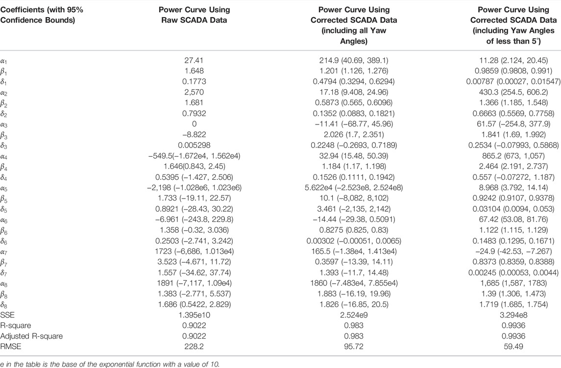
When using the Gaussian fitting method, the coefficient n in Eq. 10 is set to be 8, the nonlinear least square fitting method is employed, and the algorithm is “trust region”. The method has been integrated into the curve fitting toolbox of MATLAB. In the specific settings, the minimum change in coefficients for finite difference Jacobians is 1 × 10⁻⁸, the maximum change in coefficients for finite difference Jacobians is 0.1, the maximum number of function (model) evaluations allowed is 600, the maximum number of fit iterations allowed is 400, the termination tolerance used on stopping conditions involving the function (model) value is 1 × 10⁻⁶, the termination tolerance used on stopping conditions involving the coefficients is 1 × 10⁻⁶. Also, the “center and scale” method is selected to use. When using this method, the abscissa of the data points to be fitted is changed by Eq. 11 in MATLAB, that is

$v^{\prime }=\frac{v-\text{mean}\left(v\right)}{\text{std}\left(v\right)}(11)$

Then, Eq. 10 can be rewritten as

$P=f\left(\frac{v-\text{mean}\left(v\right)}{\text{std}\left(v\right)}\right)={\displaystyle \sum _{i=1}^n{\alpha }_i\cdot e^{-{\left[\frac{\left(x^{\prime }-{\beta }_i\right)}{{\delta }_i}\right]}^2}}(12)$

Figure 5 shows the power curve based on Gaussian fitting in three different scenarios. Figure 5A shows the wind-power scatters and the fitting curve using the raw wind speed data. Here, the selected wind speed ranges from 3 m/s to 13 m/s, and 0 values are excluded. The wind speed interval of 0.1 m/s is used to draw the fitting curve. Although the scatterplot covers a wide range, the trend of the fitting curve is consistent with the design law. It also illustrates that the curve fitting method is suitable. Figure 5B shows the wind-power scatters and the fitting curve using the corrected wind speed data in which all the yaw angles are contained. The range of wind-power scatterplot is significantly reduced after the wind speed correction. This shows that the wind speed correction is reasonable. It is also interesting to note that the upper contour of the wind-power scatterplot is relatively regular. In contrast, the lower contour of the wind-power scatterplot is still irregular.

FIGURE 5

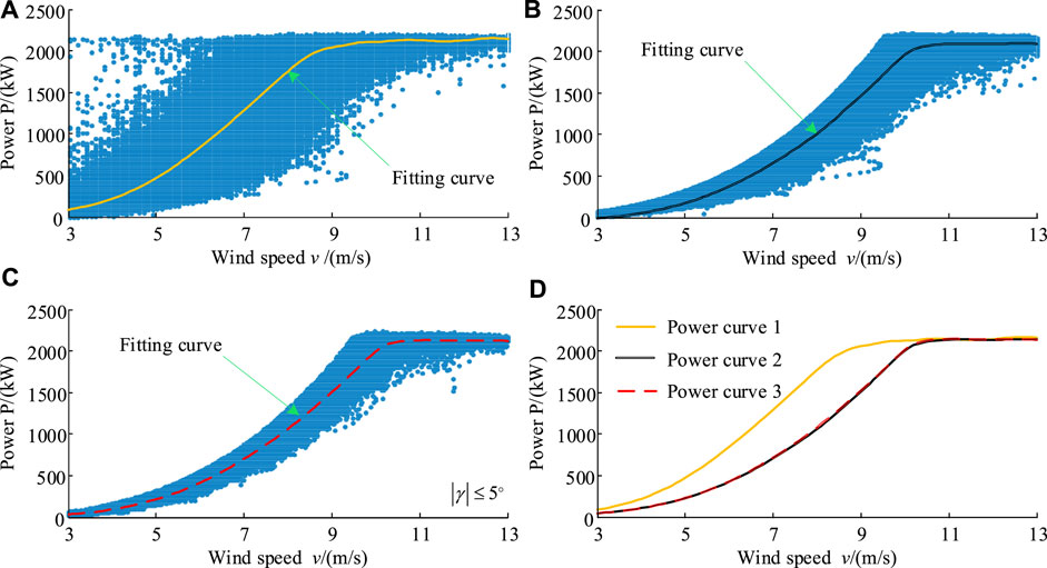
FIGURE 5. Power curve based on Gaussian fitting (WT1). (A) Wind speed /(m/s). (B) Wind speed /(m/s). (C) Wind speed /(m/s). (D) Time 400s/div.

Figure 5C shows the wind-power scatters and the fitting curve using the corrected wind speed data in which only yaw angles of less than 5° are included. For ease of comparison, the wind-power fitting curves for the three scenarios are put together in Figure 5D. Curve 1 denotes the wind-power fitting curve of scenario Ⅰ (Figure 5A), curve 2 denotes the wind-power fitting curve of scenario Ⅱ (Figure 5B), and curve 3 denotes the wind-power fitting curve of scenario Ⅲ (Figure 5C). Table 1 shows the fitting coefficients and goodness of the power curve. In different scenarios, the fitting coefficient is different. For scenario Ⅰ, x is normalized by mean 6.258 and std 2.071; for scenario Ⅱ, x is normalized by mean 7.319 and std 2.367; for scenario Ⅲ, x is normalized by mean 7.487and std 2.384. In Figure 5D, curve 2 and curve 3 are basically coincident, and both are separated from curve 1. This shows that a wider yaw angle does not significantly affect wind-power fitting. This is because there are positive and negative yaw angles, and the effects of positive and negative yaw angles on the wind-power curve cancel each other out. In curve 1, the critical wind speed at which the wind turbine reaches the rated output power is less than that in curve 2 (curve 3). What needs explanation is that taking into account the actual operating characteristics of wind turbines, in Figure 5C, data with power coefficients greater than 0.593 and less than 0.15 are excluded.

TABLE 1

TABLE 1. Fitting coefficients and goodness of the power curve (WT1).

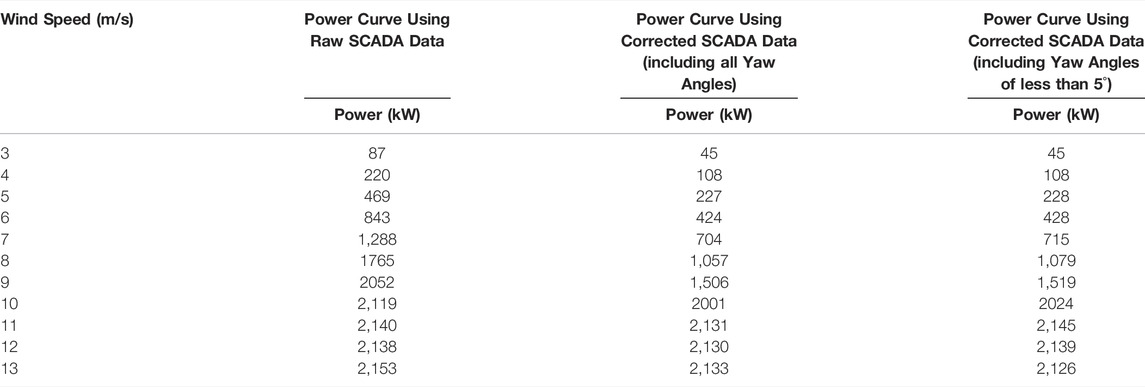
Table 2 gives wind speed and the corresponding power based on the fitting curve. In curve 1, when the wind speed is 9 m/s, the power of the generator is 2052 kW. Further, it can be found by calculating the curve fitting expression that when the wind speed is 8.7 m/s, the power of the wind turbine reaches 2000 kW. In curve 2, the wind speed is about 10 m/s which corresponds to the power of 2000 kW. Likewise, the wind speed is about 10 m/s which corresponds to the power of 2000 kW in curve 3. According to the wind turbine manufacturer, the designed rated wind speed is about 10.5 m/s. From this information, it is obvious that curve 2 and curve 3 fit better. This further shows that the wind speed correction is effective.

TABLE 2

TABLE 2. Wind speed and the corresponding power based on fitting curve (WT1).

What needs to be further explained is that the fitted critical wind speed is 10 m/s, which is different from the 10.5 m/s designed by the manufacturer. There are several reasons to consider. The design value of a wind turbine is calculated based on a specific service condition, while the actual service conditions are variable, such as wind speed fluctuations, temperature changes, humidity changes, and so on. Because of the complexity of wind turbines, the physical model must be simplified in design, which leads to the difference between the physical model and the actual model. Because of the limitation of the level of the manufacturer, there are some differences between the manufactured turbine and the designed turbine. From the operating results, the constant power output of the wind turbine is not just 2000 kW, but more than 2000 kW. Generally, the wind-power curve after the wind speed correction is more in line with the actual situation. This is applicable to the performance evaluation of wind turbines in wind farms.

Reliability Assessment of Power Curve

Power curve modeling involves the processing of some parameters. If there is uncertainty (deviation) in the parameter value, it will affect the accuracy of power curve modeling. For example, the historical air relative humidity is used for the power curve modeling, which is not recorded directly in the SCADA system and can only be extracted by consulting the data from other websites or database and is the humidity data in the larger region, which is bound to have some differences with the real humidity data. Although the temperature is directly recorded in SCADA data, it is only the temperature data recorded near the wind tower in wind farms. For mountain wind farms, significant differences in distance and altitude can also cause temperature data bias. In Eq. 4, the parameter $v_d$ denotes the wind speed in the wind rotor plane. However, the actual wind speed used is the measured result by the anemometer on the nacelle. Therefore, the deviation between the measured wind speed and the theoretical wind speed will also affect the accuracy of the power curve.

It should be noted that none of the above deviations are due to errors of the sensor itself. In other words, even if the sensors are very accurate, these deviations still exist. In another scenario, the effect of the sensor’s error should also be considered. Specifically, the two direct parameters for power curve modeling are wind speed and power, both in the SCADA system. The reliability of wind speed data and power data in the SCADA system should be judged. In this way, the actual power curve can be obtained better.

· Uncertainty effect of air humidity, air temperature, air density, and wind speed

From Eq. 7, the deviation of relative humidity will affect the calculation of air density and then affect the calculation of wind speed in Eq. 6. If the air humidity has a ${\delta }_{\text{p}}\%$ deviation, the effect on the air density can be written as

$\frac{\widehat{\rho }}{\rho }=\left[\frac{{\mathrm{P}}_0{e}^{\frac{-gM\left(h-h_0\right)}{R\cdot T_k}}-{\widehat{\mathrm{P}}}_{\mathrm{V}}}{R_d\cdot T_{\mathrm{K}}}+\frac{{\widehat{\mathrm{P}}}_{\mathrm{V}}}{R_v\cdot T_K}\right]/\rho (13)$

where, $\rho$ is the actual air density; $\widehat{\rho }$ is the air density with some deviation ${\text{P}}_{\text{V}}=6.1078\times {10}^{\frac{7.5T_C}{T_C+237.3}}\cdot \text{RH}\left(1+{\delta }_{\text{p}}\%\right)$.

If the air temperature has a deviation $\text{Δ}T$, the effect on the air density can be written as

$\frac{\widehat{\rho }}{\rho }=\left[\frac{{\mathrm{P}}_0{e}^{\frac{-gM\left(h-h_0\right)}{R\cdot \left(T_k+\mathrm{\Delta }T\right)}}-{\widehat{\mathrm{P}}}_V}{R_d\cdot \left(T_K+\mathrm{\Delta }T\right)}+\frac{{\widehat{\mathrm{P}}}_V}{R_v\cdot \left(T_K+\mathrm{\Delta }T\right)}\right]/\rho (14)$

where, ${\widehat{\text{P}}}_{\text{V}}=6.1078\times {10}^{\frac{7.5\left(T_C+\mathrm{\Delta }T\right)}{T_C+237.3+\mathrm{\Delta }T}}\cdot \text{RH}$.

From Eq. 7, if the air density has a deviation $\mathrm{\Delta }\rho$, the effect on the wind speed calculation can be written as

$\frac{{\widehat{\mathit{v}}}_1}{v_1}=\left[\frac{P}{2\left(\rho +\mathrm{\Delta }\rho \right)S{v}_d^2}+v_d\right]/v_1(15)$

If the measured wind speed $v_d$ has a deviation $\mathrm{\Delta }{v}_d$ with the actual wind speed in the wind rotor plane, the effect on the wind speed calculation can be written as

$\frac{{\widehat{\mathit{v}}}_1}{v_1}=\left[\frac{P}{2\rho S{\left(v_d+\mathrm{\Delta }{v}_d\right)}^2}+\left(v_d+\mathrm{\Delta }{v}_d\right)\right]/v_1(16)$

Figure 6 shows the calculation results of the uncertainty effect of environmental parameters. In Figure 6A, the basic value of relative humidity is set to 0.8, and then given a deviation from -20 to 20%, the air density changes under different temperature conditions are shown. The higher the temperature is, the more significant the effect on air density is. Overall, deviations in relative humidity have little effect on air density. For example, at a temperature of 20°, a 20% deviation in humidity has only an effect of 0.15%. In Figure 6B, the temperature deviation is set in the range of -3°C to +3°C, and the fitting curves of air density change under three temperature base values are given. The three fitting curves basically coincide. Furthermore, the higher the temperature is, the lower the air density is. The numerical results show that the air density changes by 1.1% when the temperature deviation is 3°C. In Figure 6C, the basic air density value is 1.2 kg/m³, the turbine power is set to be 2000 kW, and the given deviation ranges from -0.15 kg/m³ to 0.15 kg/m³. When the measured wind speed $v_d$ is different, the effect of air density deviation on the corrected wind speed is slightly different. The smaller the measured wind speed $v_d$, the larger the corresponding effect. When $v_d$ is 10 m/s and the air density deviation is 0.15 kg/m³, the effect on the corrected wind speed is 1.15%. In Figure 6D, the given deviation of the measured wind speed ranges from -0.5 m/s to 0.5 m/s. Relatively, the deviation of the measured wind speed significantly influences the calculation result of the corrected wind speed. For instance, when the measured wind speed $v_d$ is 10 m/s, the maximum effect on the corrected wind speed is 3.5%.

· Reliability assessment of wind speed and power data

FIGURE 6

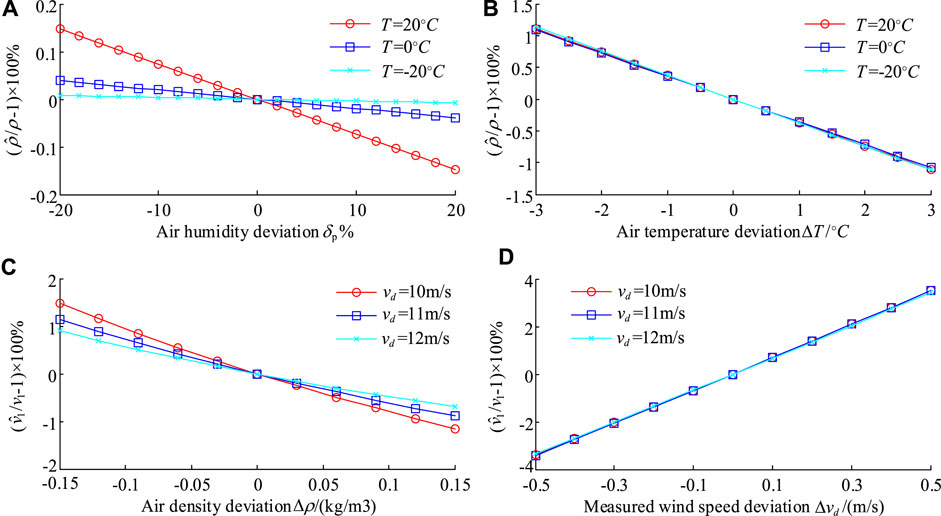
FIGURE 6. Uncertainty effect of air humidity, air temperature, air density, and wind speed. (A) Air humidity deviation p%. (B) Air temperature deviation T /C. (C) Air density deviation /(kg/m3). (D) Measured wind speed deviation v d /(m/s).

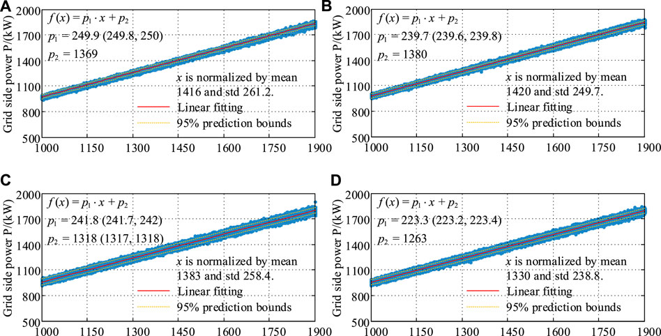
In the SCADA data, the generator side power (P_gen) and the grid side power (P_grid) of the converter are recorded simultaneously. It is believed that the two data will not have synchronously deviated. Therefore, the reliability can be judged by comparing the relationship between the two sets of power data. Specifically, the generator side power is given by the abscissa, and the grid side power is provided by the ordinate. The linear fitting curve and equation are provided by the scatter relationship between the two. In Figure 7, the generator-side power and grid-side power of the four wind turbines are shown. For the convenience of analysis, only the data of the generator side power between 1,000 kW and 1900 kW is selected. The relationship scatters between the two are very close and linearly related. In Table 3, the generator side power and grid side power based on the fitting equation are given, where the grid side power is calculated using the fitting equation. For a given generator side power, the calculated grid side power is different for different wind turbines. Overall, the power data of WT1 and WT2 are close to each other, while the power data of WT3 and WT4 are close to each other. To quantify the differences between different wind turbines, a relative difference $\left(\text{max}\left(P_{grid}\right)-\text{min}\left(P_{grid}\right)\right)/P_{gen}$ is given in row 5 of Table 2. Under different power conditions, the values are basically the same, which shows that the relationship between generator side power and grid side power is stable. Moreover, the maximum grid side power always appears on WT2, and the minimum grid side power always appears on WT4.

FIGURE 7

FIGURE 7. Generator side power and grid side power. (A) WT1; (B) WT2; (C) WT3; (D) WT4.

TABLE 3

TABLE 3. Generator side power and grid side power based on fitting equation (kW).

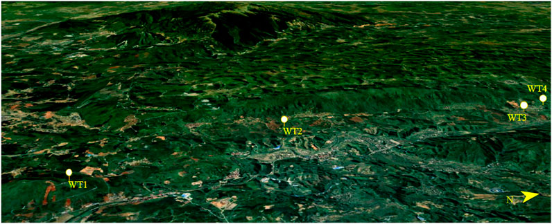
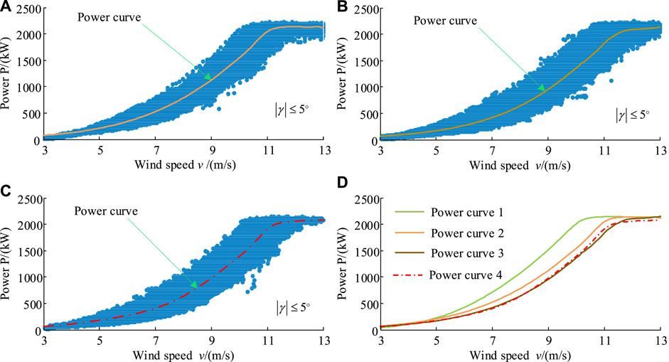
To analyze the power curve of wind turbines more comprehensively, four wind turbines in a mountain wind farm in south China are investigated. The specific topography of the wind farm is shown in Figure 8. Their power curves are shown in Figure 9. Since Figure 5 has given the power scatter of 1# wind turbine (WT1), Figures 9A–C only show the power scatters of 2# (WT2), 3# (WT3), and 4# (WT4). Figure 9D shows the power fitting curves of 4 wind turbines. The power curves of the four wind turbines do not entirely overlap, which seems to mean that although they are of the same type, the actual operating performance is always different. Of course, this difference cannot be ruled out due to the uncertainty of the data used. The benefit of obtaining these power curves is to provide a basis for further analysis of the performance of wind turbines. WT3 and WT4 are the closest among these power curves, WT2 is the next, and WT1 has the farthest deviation. In terms of the wind speed required to reach the designed rated power (2000 kW), WT1 is 10 m/s, WT2 is 10.9 m/s, WT3 is 11.4 m/s, and WT4 is 11.3 m/s. Since the design rated wind speed of the wind turbine is 10.5 m/s, WT1 is less than the rated wind speed, and the other three wind turbines are all greater than the designed rated wind speed. There may be several reasons for this phenomenon. 1) The power curve of WT1 deviates significantly from the other three wind turbines, which may be caused by the inaccurate anemometer of WT1. 2) If the measurement results of the anemometer are accurate, it is likely that the yaws of WT2, WT3, and WT4 have a large deviation, resulting in the need for greater wind speed to obtain the same power output. 3) If the previous two assumptions do not exist, then it should be caused by sensor deviation or the different performance characteristics of different wind turbines.

FIGURE 8

FIGURE 8. Four wind turbines in a mountain wind farm.

FIGURE 9

FIGURE 9. Power curve of 4 wind turbines. (A) WT2; (B) WT3; (C) WT4; (D) 4 WTs.

Conclusion

In this paper, a novel idea is proposed to obtain the actual power curve of wind turbines. A series of effective measures are taken to deal with the zero and null values in the original SCADA data, consider the comprehensive result of wind on the wind turbine power and correct the deviation between the measured wind speed and the real wind speed. The Gaussian fitting algorithm is used to fit the wind power curve; the power curve characteristics before and after the wind speed correction are compared and analyzed. Also, the characteristics of the power curves of four wind turbines are compared and analyzed. The results show that among these power curves, WT3 and WT4 are the closest, followed by WT2, and WT1 has the largest deviation from the other three wind turbines. The wind speed required for different turbines to reach the designed rated power is different from the actual power curves. Specifically, WT1 is 10 m/s, WT2 is 10.9 m/s, WT3 is 11.4 m/s, and WT4 is 11.3 m/s.

For the research topic of this paper, it is necessary to deepen it in the future further. For example, the research object of this paper is direct-drive wind turbines, and its algorithm can be transplanted to doubly-fed wind turbines or other types of wind turbines in the future. On the other hand, the power curve of wind turbines may evolve with the increase of service time, so historical SCADA data can be used to observe its historical evolution trend further. More importantly, according to the characteristics of the power curve and the actual service conditions in wind farms, the operation strategy and maintenance strategy of wind turbines can be further studied.

Data Availability Statement

The original contributions presented in the study are included in the article/Supplementary Materials, further inquiries can be directed to the corresponding author.

Author Contributions

JD contributing to the conception and writing the manuscript. HZ data processing and analysis. FZ structure design and paragraph organization. HC writing assistance and English proofreading. ML data processing and analysis assistance.

Funding

This work is supported by the National Natural Science Foundation of the People’s Republic of China (grant number 52075164, 51975535) and the science and technology innovation Program of Hunan Province (grant number 2021RC4038).

Conflict of Interest

The authors declare that the research was conducted in the absence of any commercial or financial relationships that could be construed as a potential conflict of interest.

Publisher’s Note

All claims expressed in this article are solely those of the authors and do not necessarily represent those of their affiliated organizations, or those of the publisher, the editors and the reviewers. Any product that may be evaluated in this article, or claim that may be made by its manufacturer, is not guaranteed or endorsed by the publisher.

Abbreviations

ANN, artificial neural network; GP, Gaussian process; MAF, moving average filtering; MLE, maximum likelihood estimation; NSFM, non-symmetric fuzzy means; SCADA, supervisory control and data acquisition; SLF, standard logistic functions; TI, turbulence intensity; WT, wind turbine; WTPC, wind turbine power curve; WWEA, World Wind Energy Association.

References

Astolfi, D., Castellani, F., Lombardi, A., and Terzi, L. (2021). Multivariate SCADA Data Analysis Methods for Real-World Wind Turbine Power Curve Monitoring. Energies 14 (4), 1105. doi:10.3390/en14041105

CrossRef Full Text | Google Scholar

Astolfi, D., Malgaroli, G., Spertino, F., Amato, A., Lombardi, A., and Terzi, L. (2021). “Long Term Wind Turbine Performance Analysis through SCADA Data: A Case Study,” in 2021 IEEE 6th International Forum on Research and Technology for Society and Industry (RTSI) (IEEE), 7–12.

CrossRef Full Text | Google Scholar

Bakir, I., Yildirim, M., and Ursavas, E. (2021). An Integrated Optimization Framework for Multi-Component Predictive Analytics in Wind Farm Operations & Maintenance. Renew. Sustain. Energy Rev. 138, 110639. doi:10.1016/j.rser.2020.110639

CrossRef Full Text | Google Scholar

Carullo, A., Ciocia, A., Malgaroli, G., and Spertino, F. (2021). An Innovative Correction Method of Wind Speed for Efficiency Evaluation of Wind Turbines. ACTA IMEKO 10 (2), 46–53. doi:10.21014/acta_imeko.v10i2.1037

CrossRef Full Text | Google Scholar

Ciulla, G., D’Amico, A., Di Dio, V., and Lo Brano, V. (2019). Modelling and Analysis of Real-World Wind Turbine Power Curves: Assessing Deviations from Nominal Curve by Neural Networks. Renew. Energy 140, 477–492. doi:10.1016/j.renene.2019.03.075

CrossRef Full Text | Google Scholar

Dai, J., Cao, J., Liu, D., Wen, L., and Long, X. (2016). Power Fluctuation Evaluation of Large‐scale Wind Turbines Based on SCADA Data. IET Renew. Power Gener. 11 (4), 395–402. doi:10.1049/iet-rpg.2016.0124

CrossRef Full Text | Google Scholar

Dai, J., Liu, D., Wen, L., and Long, X. (2016). Research on Power Coefficient of Wind Turbines Based on SCADA Data. Renew. Energy 86, 206–215. doi:10.1016/j.renene.2015.08.023

CrossRef Full Text | Google Scholar

Dai, J., Tan, Y., and Shen, X. (2019). Investigation of Energy Output in Mountain Wind Farm Using Multiple-Units SCADA Data. Appl. Energy 239, 225–238. doi:10.1016/j.apenergy.2019.01.207

CrossRef Full Text | Google Scholar

Dai, J., Yang, X., Hu, W., Wen, L., and Tan, Y. (2018). Effect Investigation of Yaw on Wind Turbine Performance Based on SCADA Data. Energy 149, 684–696. doi:10.1016/j.energy.2018.02.059

CrossRef Full Text | Google Scholar

Dai, J., Yang, X., and Wen, L. (2018). Development of Wind Power Industry in China: A Comprehensive Assessment. Renew. Sustain. Energy Rev. 97, 156–164. doi:10.1016/j.rser.2018.08.044

CrossRef Full Text | Google Scholar

Dawn, S., Tiwari, P. K., Goswami, A. K., Singh, A. K., and Panda, R. (2019). Wind Power: Existing Status, Achievements and Government's Initiative towards Renewable Power Dominating India. Energy Strategy Rev. 23, 178–199. doi:10.1016/j.esr.2019.01.002

CrossRef Full Text | Google Scholar

Dhunny, A. Z., Timmons, D. S., Allam, Z., Lollchund, M. R., and Cunden, T. S. M. (2020). An Economic Assessment of Near-Shore Wind Farm Development Using a Weather Research Forecast-Based Genetic Algorithm Model. Energy 201, 117541. doi:10.1016/j.energy.2020.117541

CrossRef Full Text | Google Scholar

Gao, L., and Hong, J. (2021). Data-driven Yaw Misalignment Correction for Utility-Scale Wind Turbines. J. Renew. Sustain. Energy 13 (6), 063302. doi:10.1063/5.0056671

CrossRef Full Text | Google Scholar

Gonzalez, E., Stephen, B., Infield, D., and Melero, J. J. (2017). On the Use of High-Frequency SCADA Data for Improved Wind Turbine Performance Monitoring. J. Phys. Conf. Ser. 926, 012009. doi:10.1088/1742-6596/926/1/012009

CrossRef Full Text | Google Scholar

Gonzalez, E., Stephen, B., Infield, D., and Melero, J. J. (2019). Using High-Frequency SCADA Data for Wind Turbine Performance Monitoring: A Sensitivity Study. Renew. Energy 131, 841–853. doi:10.1016/j.renene.2018.07.068

CrossRef Full Text | Google Scholar

Hansen, M. O. L. (2008). Aerodynamics of Wind Turbines. 2nd Edition. Eaethscan, UK and USA.

Google Scholar

Karamichailidou, D., Kaloutsa, V., and Alexandridis, A. (2021). Wind Turbine Power Curve Modeling Using Radial Basis Function Neural Networks and Tabu Search. Renew. Energy 163, 2137–2152. doi:10.1016/j.renene.2020.10.020

CrossRef Full Text | Google Scholar

Kim, D.-Y., Kim, Y.-H., and Kim, B.-S. (2021). Changes in Wind Turbine Power Characteristics and Annual Energy Production Due to Atmospheric Stability, Turbulence Intensity, and Wind Shear. Energy 214, 119051. doi:10.1016/j.energy.2020.119051

CrossRef Full Text | Google Scholar

Li, L., Mu, X., Macfarlane, C., Song, W., Chen, J., Yan, K., et al. (2018). A Half-Gaussian Fitting Method for Estimating Fractional Vegetation Cover of Corn Crops Using Unmanned Aerial Vehicle Images. Agric. For. Meteorology 262, 379–390. doi:10.1016/j.agrformet.2018.07.028

CrossRef Full Text | Google Scholar

Lydia, M., Kumar, S. S., Selvakumar, A. I., and Prem Kumar, G. E. (2014). A Comprehensive Review on Wind Turbine Power Curve Modeling Techniques. Renew. Sustain. Energy Rev. 30, 452–460. doi:10.1016/j.rser.2013.10.030

CrossRef Full Text | Google Scholar

Manobel, B., Sehnke, F., Lazzús, J. A., Salfate, I., Felder, M., and Montecinos, S. (2018). Wind Turbine Power Curve Modeling Based on Gaussian Processes and Artificial Neural Networks. Renew. Energy 125, 1015–1020. doi:10.1016/j.renene.2018.02.081

CrossRef Full Text | Google Scholar

Marčiukaitis, M., Žutautaitė, I., Martišauskas, L., Jokšas, B., Gecevičius, G., and Sfetsos, A. (2017). Non-linear Regression Model for Wind Turbine Power Curve. Renew. Energy 113, 732–741. doi:10.1016/j.renene.2017.06.039

CrossRef Full Text | Google Scholar

Mehrjoo, M., Jafari Jozani, M., and Pawlak, M. (2021). Toward Hybrid Approaches for Wind Turbine Power Curve Modeling with Balanced Loss Functions and Local Weighting Schemes. Energy 218, 119478. doi:10.1016/j.energy.2020.119478

CrossRef Full Text | Google Scholar

Mehrjoo, M., Jafari Jozani, M., and Pawlak, M. (2020). Wind Turbine Power Curve Modeling for Reliable Power Prediction Using Monotonic Regression. Renew. Energy 147, 214–222. doi:10.1016/j.renene.2019.08.060

CrossRef Full Text | Google Scholar

Pandit, R. K., Infield, D., and Kolios, A. (2020). Gaussian Process Power Curve Models Incorporating Wind Turbine Operational Variables. Energy Rep. 6, 1658–1669. doi:10.1016/j.egyr.2020.06.018

CrossRef Full Text | Google Scholar

Rogers, T. J., Gardner, P., Dervilis, N., Worden, K., Maguire, A. E., Papatheou, E., et al. (2020). Probabilistic Modelling of Wind Turbine Power Curves with Application of Heteroscedastic Gaussian Process Regression. Renew. Energy 148, 1124–1136. doi:10.1016/j.renene.2019.09.145

CrossRef Full Text | Google Scholar

Saint-Drenan, Y.-M., Besseau, R., Jansen, M., Staffell, I., Troccoli, A., Dubus, L., et al. (2020). A Parametric Model for Wind Turbine Power Curves Incorporating Environmental Conditions. Renew. Energy 157, 754–768. doi:10.1016/j.renene.2020.04.123

CrossRef Full Text | Google Scholar

Seo, S., Oh, S.-D., and Kwak, H.-Y. (2019). Wind Turbine Power Curve Modeling Using Maximum Likelihood Estimation Method. Renew. Energy 136, 1164–1169. doi:10.1016/j.renene.2018.09.087

CrossRef Full Text | Google Scholar

Sun, H., Qiu, C., Lu, L., Gao, X., Chen, J., and Yang, H. (2020). Wind Turbine Power Modelling and Optimization Using Artificial Neural Network with Wind Field Experimental Data. Appl. Energy 280, 115880. doi:10.1016/j.apenergy.2020.115880

CrossRef Full Text | Google Scholar

Villanueva, D., and Feijóo, A. (2018). Comparison of Logistic Functions for Modeling Wind Turbine Power Curves. Electr. Power Syst. Res. 155, 281–288. doi:10.1016/j.epsr.2017.10.028

CrossRef Full Text | Google Scholar

Virgolino, G. C. M., Mattos, C. L. C., Magalhães, J. A. F., and Barreto, G. A. (2020). Gaussian Processes with Logistic Mean Function for Modeling Wind Turbine Power Curves. Renew. Energy 162, 458–465. doi:10.1016/j.renene.2020.06.021

CrossRef Full Text | Google Scholar

Xu, N., Sheng, L., Chen, C., Li, Y., Su, T., Zhao, B., et al. (2019). Application of Gaussian Fitting to the Fast Search of Pulsar Periodic. Optik 198, 163253. doi:10.1016/j.ijleo.2019.163253

CrossRef Full Text | Google Scholar

Yesilbudak, M. (2018). Implementation of Novel Hybrid Approaches for Power Curve Modeling of Wind Turbines. Energy Convers. Manag. 171, 156–169. doi:10.1016/j.enconman.2018.05.092

CrossRef Full Text | Google Scholar