Anomaly Detection of Hydropower Units Based on Recurrent Neural Network

Anomaly detection for hydraulic turbine unit has an important role in hydropower system. In hydropower systems, different components will produce n-dimensional heterogeneous time series with different characteristics at all times. Due to the characteristic evolution and time dependence, vibration-based anomaly detection for hydraulic turbine unit is extremely challenging. In this paper, we propose a conditional quantile regression based recurrent neural network (QRNN), which models the time dependence and probability distribution between random variables. The proposed method aims to extract the actual representation patterns from the fitted models and it can effectively detect anomalies in the non-uniform time series of feature evolution. The experimental results show that the proposed method has better accuracy in anomaly detection (error reduction by 34%) than the traditional method, and saves at least 25.6% of execution time.

1 Introduction

In order to control the stability and security, data analysis and detection methods play an important role in power systems (Liu et al., 2017; Xiong et al., 2019; Xiong et al., 2021). Different from the wind power system (Liu et al., 2020), the operation process of a hydropower unit is complex. According to the statistics, the vibration signal of the unit can reflect more than 80% of the fault characteristics. Therefore, we propose to detect the fault of hydropower turbine unit based on mining the vibration signal data in this paper. Due to highly nonlinear, instability and time-varying characteristics of the vibration signal data of the hydraulic turbine unit, it is difficult to be modeled precisely. At present, the non-stationary vibration signal processing methods include short-time Fourier transform, Mode Decomposition and so on. In order to solve the problems of empirical mode decomposition on mathematical theory, Konstantin et al. (Iyer et al., 2016) proposed variational mode decomposition method. Assuming that the signal is composed of modal functions with different center frequencies, it is decomposed by self-adaptive and quasi-orthogonal methods in the variational framework. Breiman et al. (Breiman, 2001) proposed the random forest theory. Based on decision tree, this method generates several decision trees by randomly feature selection and samples. After each decision tree is trained separately, the final sample category is voted on. However, they are not suitable for processing the multivariate vibration time series data of hydraulic turbine unit.

Extreme value theory (EVT) (Xu et al., 2018), Peak over-threshold (POT) (Hundman et al., 2018), and distance-based (Dragomiretskiy and Zosso, 2013) can be used for time series anomaly detection (Wu et al., 2014). All these methods may involve a large number of distribution assumptions, parameter adjustments, and heavy calculations in the conversion process. This may increase the calculation cost. Although there are many studies on anomaly detection (Mehrotra et al., 2017), they either focus on deterministic methods (Filonov et al., 2016) or random methods (Dasgupta and Osogami, 2017; Lai et al., 2018), and ignore time dependence of the time series (Guha et al., 2016). In (Manzoor et al., 2018), the goal is to identify independent anomalous objects rather than identifying anomalous time series patterns based on their time dependence. In time series modeling, historical observations are very important for understanding current data. Therefore, it is better to use a sequence of observations: X_(t-T), X_(t-T+1), …, X_t rather than X_t to calculate the anomaly score in time series.

Vector auto regression (VAR) and support vector regression (SVR) can be applied to multivariate time series (Lai et al., 2018). However, many of these models are difficult to scale up and include exogenous variables (Liu et al., 2020). Supervised methods (Laptev et al., 2015; Shipmon et al., 2017) require labeled data for model training, and can only identify known types of anomalies. The unsupervised method does not need to label the data, which can be divided into two categories: the deterministic model and random model. For deterministic model. In order to capture both the long-term dynamics and short-term effects simultaneously, the non-linear dynamics modeling, long short term memory (LSTM) methods (Hochreiter and Schmidhuber, 1997; Gers et al., 2000; Borovykh et al., 2017; Grob et al., 2018) have been proposed for forecasting events based on sequence models. For deterministic model, (Filonov et al., 2016) proposed a LSTM-based predictive models to detect spacecraft anomalies. Although LSTMs are deterministic and have no random variables, they can handle the time dependence of heterogeneous time series. For random model, recurrent neural network (Dasgupta and Osogami, 2017; Lai et al., 2018) is used for time series anomaly detection. Auto-encoder-based methods are used for time series anomaly detection in (Boudiaf et al., 2016; Xu et al., 2018). Variants of convolution and recurrent neural networks are used for modeling temporal patterns (Calvo-Bascones et al., 2021). Deep convolutional neural networks (Kim, 2014; Yang et al., 2015) have been used for time series human activity recognition. Memory guided normality for anomaly detection is proposed in (Park et al., 2020). Deep learning based anomaly detection methods for video and industrial control system are proposed in Wang et al. (2020) and Nayak et al. (2021), respectively. The deep neural network (Sen et al., 2019), (Salinas et al., 2017) has been proposed to high dimensional time series forecasting, however, it is limited to training on entire time series and then perform multi-step ahead forecast which is practically computational resource demanding in feature evolving heterogeneous time series. Recently, (Pang et al., 2021) give a survey of deep learning methods for anomaly detection. However, in the hydraulic turbine system, different subsystems and parts will produce n-dimensional heterogeneous time series with different characteristics at all times. This will form a heterogeneous time series of feature evolution.

In this paper, we propose a quantile regression (Geraci and Bottai, 2007) based recurrent neural network (QRNN) for anomaly detection of hydropower units. The proposed method can explicitly model the temporal dependence among stochastic variables with properly estimated probability distributions. Considering the feature evolution of heterogeneous time series, the most difficult part in this method is still how to detect anomalies. The most intuitive way to verify the reliability of the detection model is to find the correct estimated distribution probability. The higher the probability, the higher the confidence. But this does not mean higher accuracy. The proposed method aims to extract the actual representational patterns from the fitted models, thereby studying their reconstruction error probability distribution by using a conditional quantile regression method to limit mistakes when it is forced to make decision on normality by guidance of principled uncertainty estimates. Inspired by the distribution assumptions-free QR (Koenker and Bassett Jr, 1978; Koenker and Machado, 1999; Koenker and Hallock, 2001) build on asymmetric laplace distribution (Kotz et al., 2001), we proposed QRNN to model the conditional distribution $P(\widehat{y_t}|X_{t-T},X_{t-T+1},\dots ,X_t)$, where $\widehat{y_t}$ is the predicted value. The contributions of this paper can be summarized as follows:

• According to the characteristics of hydraulic turbine data, we propose a quantile regression based recurrent neural network for anomaly detection, which can model temporal dependencies and stochasticity explicitly in vibration time series data. And it can study the reconstruction error probability distribution by using a conditional quantile regression method.

• We propose an incremental online method to update the co-evolving heterogeneous for multiple streaming data.

• We propose to apply stochastic methods to detect anomalies in heterogeneous time series with feature evolution, which is proved robust and powerful in the experiment.

The rest of this paper is organized as follows. In Section 2, we introduce the problem and the related model used in this paper. In Section 3, we describe the proposed method in detail. In Section 4, we conduct several experiments to evaluate the advantage of the proposed method. At the end, we conclude the paper in Section 5.

2 Problem and Model

2.1 Formal Description of the Problem

Formalize the anomaly detection problem in the feature evolution time series, [T₀, T) represents the observation window of the observed event. In general, it can be assumed that T₀ = 0. Each feature F uses a continuous time stamp sequence T_u = t₁, …, t_n. X_t−T:t ∈ R^M×(T+1) represents the observation sequence X_t−T, X_t−T+1, …, X_t. $\widehat{y}$ and y represents the predicted value and the true value. L represents the loss function. In the problem of time series anomaly detection, past historical observations are very important for understanding and capturing the dynamic patterns in the current data stream. We use the observation sequence X_t−T:t to calculate the anomaly score of X_t. Given X = x₁, …, x_N, where N is the length of the vector x. The observation x_t is the N-dimensional vector $x_t=[x_t^1,\dots ,x_t^N]$ and X ∈ R^M×N at time t(t ≤ N). According to the past historical observation data X_t−T:t, the problem of anomaly detection in vibration time series data of hydraulic turbine unit is formally defined as follows.

Problem: Given the historical observation sequence represented by the time series in the order given as X_t−T:t, where t is the current time point, report an anomaly score for a given current data point X_t instantly at any time.

2.2 Long Short-Term Memory

LSTM is a kind of deep recurrent neural network. It is widely used in time series. LSTM realizes the memory function in time through the opening and closing of the door. It can effectively solve the problem of gradient disappearance and gradient explosion in general situations. The key is to introduce a gating unit system. The system stores historical information through the internal memory unit-cell state unit. Different gates can make the network know when to forget historical information, when to update cells status dynamically. Cells are cyclically connected to each other, instead of hidden units in the general cyclic network. If the input gate sigmoid allows new information input, its value can be added to the state. The state unit has linear self-circulation. Its weight is controlled by the forget gate. The output of the cell can be closed by the output gate. The status unit can also be used as an additional input for the gating unit.

$f_t=\sigma \left(w_f\ast \left[C_{t-1},Z_t,h_{t-1}\right]+b_f\right)(1)$

$i_t=\sigma \left(w_i\ast \left[C_{t-1},Z_t,h_{t-1}\right]+b_i\right)(2)$

$C_t=f_t\ast C_{t-1}+i_t\ast RELU\left(w_c\ast \left[Z_t,h_{t-1}\right]+b_c\right)(3)$

$o_t=\sigma \left(w_o\ast \left[C_t,Z_t,h_{t-1}\right]+b_o\right)(4)$

$h_t=o_t\ast RELU\left(C_t\right)(5)$

Here f, i, o, h, C, c, w, Z, b, σ() respectively represents forget gate, input gate, output gate, hidden state vector, unit state vector, weight matrix, feature vector, bias vector and sigmoid function. In this paper, we select to use LSTM due to the following features: 1) it is able to support end to end modeling; 2) it is easy to incorporate exogenous; 3) it is powerful in feature extraction for vibration time series data of hydraulic turbine unit.

3 The Proposed Method

3.1 The Architecture of QRNN

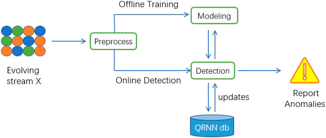
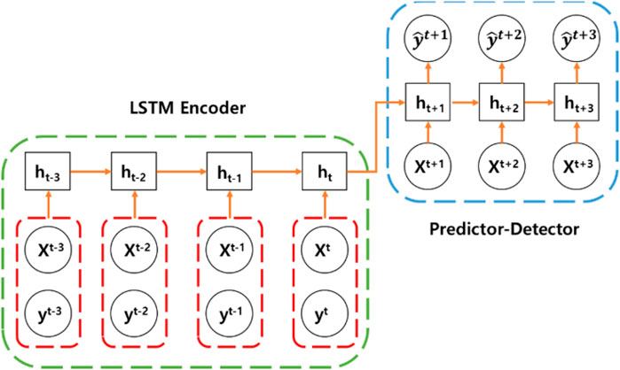
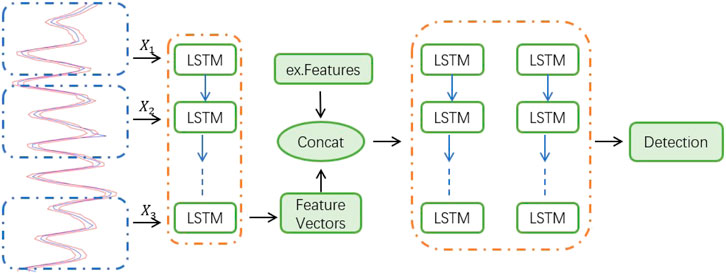
This paper propose to combine LSTM and conditional quantile regression to model explicitly temporal dependencies and stochasticity in vibration time series data of hydraulic turbine unit. The overall structure of QRNN consists of two parts: 1) offline training 2) online anomaly detection. As shown in Figure 2, the proposed neural network is composed of two recurrent neural networks, such as the LSTM encoder and predictor-detector network. It can be considered as f = pd(e(h_t, (x,y)_t)) where f is the predicted scores, x_t and y_t are the input variables, h_t is the encoder state, e(.) is an encoder and pd(.) is the predictor-detector network. The LSTM encoder is trained to extract useful temporal and non-linear patterns contained in vibration time series data, which can be used to guide the predictor-detector network of anomaly detection. If exogenous variables are available, they can get concatenated with extracted feature vectors from the LSTM encoder and used as input to the predictor-detector network. The predictor-detector network consists of an LSTM and dense layers for output prediction. The training process can be carried out daily training according to business needs, such as once a week or once a month. The offline part is composed of preprocessing sub-module (shared by online and offline modules) and start-up sub-module. The online part consists of real-time detection and update sub-modules. The data is preprocessed in the preprocessing module. The data is divided into sequences through a sliding window of length T. The startup module builds the model and deploys it to memory after training, testing, and verification. The fitted model can now perform real-time anomaly detection. In streaming or online settings, new observations after preprocessing (such as X_t at time t) can be sent to the detection module and provide anomaly scores. If the abnormal score of X_t is lower or higher than the abnormal threshold, X_t is marked as abnormal. The update of sub-module will update the parameters of each operation in QRNN db. The overall structure is shown in Figure 1.

FIGURE 1

FIGURE 1. The proposed neural network model with LSTM encoder and predictor-detector network.

FIGURE 2

FIGURE 2. The overall structure of QRNN.

QRNN is composed of LSTM encoder and prediction-detector network. The network can essentially be regarded as a large neural network, expressed as f = pd(e(h_t, (x,y)_t)), where f is the prediction score, x_t and y_t are input variables, h_t is the state of the encoder, e(.) is the ana encoder, and pd(.) is the prediction-detection network. The trained LSTM encoder can extract useful time and nonlinear dynamic patterns contained in the heterogeneous time series of feature evolution. These patterns can be used to guide the prediction-detection network to perform anomaly detection.

If exogenous variables are available, they can be connected with the feature vector extracted from the LSTM encoder and used as input to the predictor-detector network. This is because in reality, it is not necessary to observe all the content needed to predict the output through the input. After the LSTM encoder network is trained, the output from the last cell state is sent to the prediction-detection network. This is also the training prediction score evolution data stream ${\widehat{y}}_{t+M:t}=pd(h_{t-T},X_{t+M:t})$, where h(.) is the hidden coding state, as shown in Figure 3. The proposed QRNN prediction-detection network consists of an LSTM layer and a fully connected output prediction layer. The last dense layer is modeled as three outputs and three loss functions. One for the desired fitting model. The other two are used to guide the upper and lower bounds of forecast uncertainty estimates. It is worth noting that the total loss is calculated as the sum of individual quantile losses. And the output is all quantile predictions of different quantile values defined by τ ∈ [0, 1].

FIGURE 3

FIGURE 3. QRNN architecture diagram.

3.2 Fault Detection and Loss Function

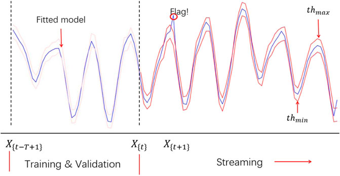
QRNN is an anomaly detector based on prediction. The anomaly detection depends on the quality of the predicted value. When predicting normal data, the probability distribution of the error can be calculated, and then used to find the maximum posterior probability estimate of the normal behavior of the test data. In order to predict more accurately, it is necessary to set thresholds for the upper and lower bounds. Beyond this threshold, data points can be marked as abnormal, as shown in Figure 4. In the deep learning regression task setting, the mean square error function is the most commonly used loss function.

${\xi }_t=y_t-\widehat{y_t}(6)$

FIGURE 4

FIGURE 4. Schematic diagram of anomaly detection.

Intuitively speaking, taking the negative power of the mean square error function approximates the Gaussian process whose mode corresponds to the mean parameter. Non-parametric distributions like conditional quantiles are very useful in quantifying uncertainty estimation in decision-making and minimizing risk.

The goal of Quantile regression (QR) is to estimate the conditional median or any other quantile of the distribution. It can be done by solving the following formula.

$\underset{\xi \in R}{\min }\sum {\rho }_r\left(y_i-\xi \right)(7)$

Where the function ρ_r(.) is the tilted absolute value function that yields the τth sample quantiles. To obtain an estimate of the conditional median function, we replace the scalar ξ by the parametric function ξ(x_i, β), which can be formulated as a linear function of parameters.

$\underset{\beta \in R}{\min }\sum {\rho }_r\left(y_i-\xi \left(x_i,\beta \right)\right)(8)$

Quantile regression learns to predict the conditional quantiles ${\widehat{y}}_{{\tau }_{t+1:M}}|(X_{t-T:t},\tau )$ for the given target distribution via formula (9), in which ${\widehat{y}}_{\tau }(.)$ is the predicted value at the given quantile.

$P\left({\widehat{y}}_{t+1:M}\le {\widehat{y}}_{{\tau }_{t+1:M}}\right)=\tau (9)$

We focus on putting weights to the distances between points on the distribution function and the fitted regression line based on the selected quantile. We select to use QR due to it has the following key features: 1) It does not make any distribution assumption on the error; 2) QR can describe the outcome variable of the entire conditional distribution; 3) QR is more robust to outliers and setting errors of the error distribution; 4) QR can expand the flexibility of parametric and non-parametric regression methods.

We set τ ∈ [0, 1] to generate the predicted value y_t+1:M with the smallest reconstruction error ξ, as shown in the formula (6) in the predictive detector network. And calculate the quantile loss of a single data point by formula (10). Because we needed a complete conditional distribution rather than a point estimate of uncertainty estimation, the average loss function L(.) on a given data distribution can be defined by formula (11), where f^W(x_t) is the fitting model under the given quantile τ, y_t and x_t are true values.

$L\left({\xi }_t|\tau \right)=\left\{\begin{array}{ccc}\tau {\xi }_t\hfill & \hfill \hfill & if{\xi }_t\ge 0\hfill \\ \left(\tau -1\right){\xi }_t\hfill & \hfill \hfill & if{\xi }_t<0\hfill \end{array}\right.(10)$

$L\left(y_t,f^W\left(x_t\right)\tau \right)=\frac{1}{L}\sum _{t=1}^{L}L\left(y_t,f^W\left(x_t\right)|\tau \right)(11)$

In the case of a loss function, the prediction-detector network is modeled as three outputs and three loss functions, with the lower quantile, the median (fitting model) and the upper quantile. At τ = 0.5, the loss function will estimate the median value instead of the average value. With the upper quantile and the lower quantile, a reliable uncertainty estimate can be provided for forecasting.

3.3 Time Series Evolution

It needs to be considered that during the operation of the turbine, the data update of each subsystem arrives in the form of a stream over time. This may include updates to existing features, or new features, as shown in Figure 1. Generally, a time series may have endogenous variables (for example, the output is a function of the previous output), or may not have exogenous variables that are not affected by other variables in the system. But the output depends on it. Most work ignores exogenous variables. But in order to improve quality and improve anomaly detection, this article introduces exogenous variables. When performing anomaly detection on the time series of various hydraulic turbines, sometimes there may be patterns that were not previously available. It deviates greatly from the training model. This may be a training data set observed in a specific mode. In general, it requires that each time a new data set is reached, the entire process of training the model must start from the beginning. For hydraulic turbine time series fault detection models, training the entire model requires a large amount of data sets and a large amount of time. In actual situations, it is impractical to keep training the model with the arrival of new data. In order to solve this problem, an online incremental update scheme is needed to provide threshold and model updates. QRNN can receive previously unavailable characteristics or evolved data points for learning, without starting from scratch, so as to mark abnormal data points and update model parameters in real time, as shown in formula (12) and (13), where th_up and th_lo are the upper and lower thresholds of the abnormal score calculated by the selected quantile, α1 and α2 are the higher and lower bounds, respectively, and $\widehat{f}(.)$ is the fitted model at the corresponding quantile (τ = 0.5 corresponds to the median).

$t{h}_{up}=\widehat{f}{\left(x_t\right)}_{\tau =\alpha 2}(12)$

$t{h}_{lo}=\widehat{f}{\left(x_t\right)}_{\tau =\alpha 1}(13)$

Based on the conditional quantile regression, with the emergence of a new data set, the confidence of the model parameter distribution will be automatically updated. The threshold value will be incrementally updated, as described in the loss function above. With this setting, QRNN can perform anomaly detection in vibration time series data of hydraulic turbine unit.

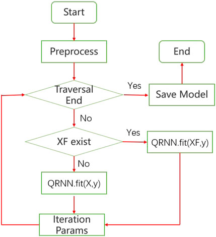
Figure 5 shows the overall algorithm of QRNN. For preprocessing, offline training, evaluation, testing and detection is performed. The fitted model $\widehat{f}(.)$ is loaded into memory ready for anomaly detection which is performed in formula (12) and (13). After the traversal is completed, the fitted model is saved to QRNNdb. QRNN is design to operate with multiple settings depending on whether exogenous features are present. During fitting, different processing needs to be performed according to whether the exogenous feature (XF) is existed. During this procedure, LSTM encoder can be used as feature extractor. Upon the arrival of vibration time series data of hydraulic turbine unit, the proposed QRNN will predict its value and seamlessly flag its anomaly score. At the same time, the model parameters will be updated. The prediction, model updates and abnormal scoring can be completed in a single pass at O(1) time complexity.

FIGURE 5

FIGURE 5. The overall algorithm of QRNN.

4 Evaluation

In order to verify the efficiency of the proposed method, we adopted the hydraulic turbine working simulation data set provided by Case Western Reserve University (CWRU) to perform the experiment and evaluation. The test bench consists of a two-horsepower motor, a torque sensor/encoder, and an electronic device for power measurement and control. The vibration data is collected by an accelerometer. The accelerometer is placed at the 12 o’clock position of the drive end and the fan end of the motor housing, which using a 16-channel DAT recorder (Smith and Randall, 2015). Experimental data of the drive end is collected at 12,000 sampling points per second and 48,000 sampling points per second. The fan data is collected at 12,000 sample per second (Boudiaf et al., 2016). The detailed attributes of the data set used in the experiment are shown in Table 1. We use python and Keras framework to build neural network. The experimental setting is CPU 2.30 GHz, 8G DDR4 3200 MHZ, and GeForce GTX 1050Ti GPU.

TABLE 1

TABLE 1. Data set attributes.

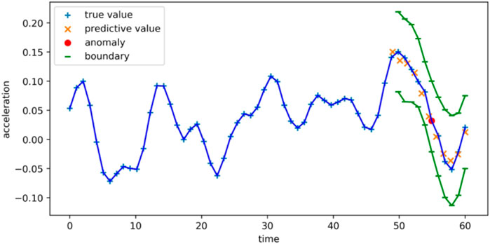
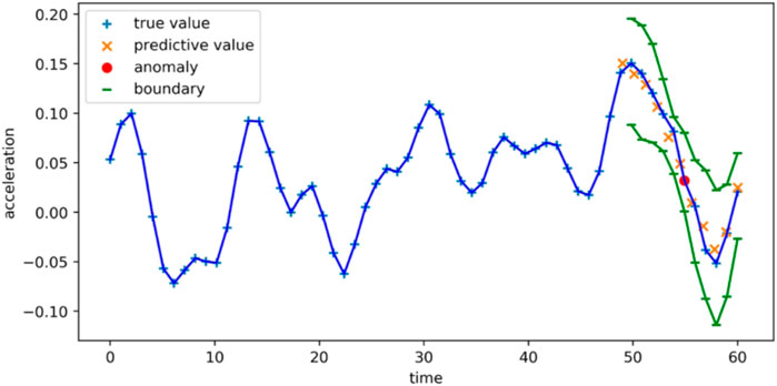
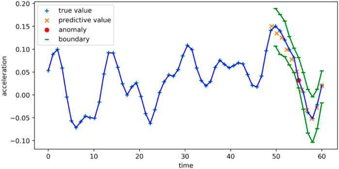
Adam optimizer is used in this method, which is an extension of SGD. In this algorithm, an adaptive gradient algorithm is introduced to adjust the learning rate. The errors of different methods on different load data sets are shown in Table 2. “1HP” in the table represents that there is a load in the device. In the QRNN method, the ability of anomaly detection largely depends on trend prediction, so the accuracy of trend prediction is very important. It can be seen from the table that the QRNN method has a greater improvement in the accuracy of trend prediction compared to other methods. Compared with the errors of CNN, GRU and BiLSTM, the QRNN method has reduced 41, 44, and 65% respectively.

TABLE 2

TABLE 2. Mean square error of trend prediction of QRNN, CNN, GRU, and BiLSTM methods on data sets under different loads.

One-dimensional CNN can be well applied to the time series analysis of sensor data (Roska and Chua, 1993) (such as gyroscope or accelerometer data). It can also be used to analyze signal data with a fixed length period (such as audio signals). It can well identify simple patterns in the data, and then use these patterns to generate more complex patterns in higher-level layers. It is generally feasible to use one-dimensional convolution to process time series. The results of CNN are shown in Figure 6.

FIGURE 6

FIGURE 6. CNN for anomaly detection.

Long short-term memory network (LSTM) was born to solve the problem of long-term dependence. As a variant of LSTM, GRU combines the forget gate and input gate into a single update gate. It mixes the cell state and the hidden state, and adds some other changes. The final model is simpler than the standard LSTM model. BiLSTM is also a variant of LSTM, which takes context into account. The results of GRU and BiLSTM are shown in Figures 7, 8, respectively.

FIGURE 7

FIGURE 7. GRU for anomaly detection.

FIGURE 8

FIGURE 8. BiLSTM for anomaly detection.

The main body of the QRNN framework is composed of LSTM encoders. LSTM network is used to solve the vanishing gradient problem. It supports end-to-end modeling and nonlinear feature extraction. In the process of training the neural network, the error margin has a direct impact on the accuracy of the model, especially the time. This is a hyper parameter and needs to be specified before training. The basis for the formulation is the convergence speed of the model and the learning accuracy of the sample. When it is too large, neither the training accuracy nor the test accuracy is high enough to meet actual needs. If it is too small, although the learning effect is more ideal, it takes a lot of time. The parameter is set between 10^–4 10^–2 generally. When the training error is lower than this value, the training is considered sufficient, and the training should be stopped. The results of the QRNN are shown in Figure 9.

FIGURE 9

FIGURE 9. QRNN for anomaly detection.

We count TP (True Positive), FP (False Positive), FN (False Negative), and TN (True Negative) based on the experimental data. TP represents the number of abnormal points marked by the neural network that are correctly marked. FP means that it is actually a normal point but is marked as an abnormal point. FN represents the number of normal points marked as abnormal points. TN represents the number of normal points that are marked correctly. We calculate the precision and recall rate of each method based on TP, FP, FN, and TN. The precision rate $(\frac{TP}{TP+FP})$ is used to measure the degree to which the method finds the right way, and the recall rate $(\frac{TP}{TP+FN})$ measures the degree to which the method is found to be complete. As shown in Table 3, it can be seen that the QRNN has the highest accuracy and recall rates (95.9%, 94.3%). In addition, although the structure of QRNN is relatively complex and the training time is longer than CNN and GRU, the overall running time (125.3 MS) is significantly shorter than them.

TABLE 3

TABLE 3. TP, FP, FN, TN value, precision, recall and running time of each method.

5 Conclusion

Anomaly detection of evolution time series is important for hydraulic turbine systems. This paper introduces a vibration-based anomaly detection method. It can deal with time-dependent and non-linear complex dynamic sequences. As a window-based anomaly detection method, it has scalability, high-efficiency stream processing efficiency and can effectively deal with the heterogeneity and randomness in the constantly changing data stream. After experimental evaluation based on real data sets, it indicates that the proposed method is fast, robust and accurate compared to the traditional anomaly detection methods.

Data Availability Statement

The data underlying this article are available in the article and in its online Supplementary Material.

Author Contributions

LX wrote the first draft of the paper, JL directed the paper writing and provided project support for the paper, and FY, GZ and the JD put forward many valuable amendments in the paper writing.

Funding

This research was funded by National Natural Science Foundation of China (52009106); Natural Science Basic Research Plan of Shaanxi Province (2019JQ-130).

Conflict of Interest

The authors declare that the research was conducted in the absence of any commercial or financial relationships that could be construed as a potential conflict of interest.

Publisher’s Note

All claims expressed in this article are solely those of the authors and do not necessarily represent those of their affiliated organizations, or those of the publisher, the editors and the reviewers. Any product that may be evaluated in this article, or claim that may be made by its manufacturer, is not guaranteed or endorsed by the publisher.

References

Borovykh, A., Bohte, S., and Oosterlee, C. W. (2017). “Conditional Time Series Forecasting with Convolutional Neural Networks,” in Proceedings of the International Conference on Artificial Neural Networks. United States: arXiv.

Google Scholar

Boudiaf, A., Moussaoui, A., Dahane, A., and Atoui, I. (2016). A Comparative Study of Various Methods of Bearing Faults Diagnosis Using the Case Western reserve university Data. J. Fail. Anal. Preven. 16, 271–284. doi:10.1007/s11668-016-0080-7

CrossRef Full Text | Google Scholar

Breiman, L. (2001). Random Forests. Machine Learn. 45, 5–32. doi:10.1023/a:1010933404324

CrossRef Full Text | Google Scholar

Calvo-Bascones, P., Sanz-Bobi, M. A., and Welte, T. M. (2021). Anomaly Detection Method Based on the Deep Knowledge behind Behavior Patterns in Industrial Components. Application to a Hydropower Plant. Comput. Industry 125, 103376. doi:10.1016/j.compind.2020.103376

CrossRef Full Text | Google Scholar

Dasgupta, S., and Osogami, T. (2017). “Nonlinear Dynamic Boltzmann Machines for Time-Series Prediction,” in The AAAI Conference on Artificial Intelligence. San Francisco, United States: AAAI Press, 31.

Google Scholar

Dragomiretskiy, K., and Zosso, D. (2013). Variational Mode Decomposition. IEEE Transactions Signal. Processing 62, 531–544. doi:10.1109/TSP.2013.2288675

CrossRef Full Text | Google Scholar

Filonov, P., Lavrentyev, A., and Vorontsov, A. (2016). Multivariate Industrial Time Series with Cyber-Attack Simulation: Fault Detection Using an Lstm-Based Predictive Data Model. NIPS.

Google Scholar

Geraci, M., and Bottai, M. (2007). Quantile Regression for Longitudinal Data Using the Asymmetric Laplace Distribution. Biostatistics 8, 140–154. doi:10.1093/biostatistics/kxj039

PubMed Abstract | CrossRef Full Text | Google Scholar

Gers, F. A., Schmidhuber, J., and Cummins, F. (2000). Learning to Forget: Continual Prediction with Lstm. Neural Comput. 12, 2451–2471. doi:10.1162/089976600300015015

PubMed Abstract | CrossRef Full Text | Google Scholar

Grob, G. L., Cardoso, Â., Liu, C., Little, D. A., and Chamberlain, B. P. (2018). “A Recurrent Neural Network Survival Model: Predicting Web User Return Time,” in Joint European Conference on Machine Learning and Knowledge Discovery in Databases (United States: Springer), 152–168.

Google Scholar

Guha, S., Mishra, N., Roy, G., and Schrijvers, O. (2016). “Robust Random Cut forest Based Anomaly Detection on Streams,” in International Conference on Machine Learning (Canada: ACM), 2712–2721.

Google Scholar

Hochreiter, S., and Schmidhuber, J. (1997). Long Short-Term Memory. Neural Comput. 9, 1735–1780. doi:10.1162/neco.1997.9.8.1735

PubMed Abstract | CrossRef Full Text | Google Scholar

Hundman, K., Constantinou, V., Laporte, C., Colwell, I., and Soderstrom, T. (2018). “Detecting Spacecraft Anomalies Using Lstms and Nonparametric Dynamic Thresholding,” in The 24th ACM SIGKDD International Conference. New York, United States: ACM, 387–395. doi:10.1145/3219819.3219845

CrossRef Full Text | Google Scholar

Iyer, A. P., Li, L. E., Das, T., and Stoica, I. (2016). “Time-evolving Graph Processing at Scale,” in The Fourth International Workshop on Graph Data Management Experiences and Systems. New York, United States: ACM, 1–6. doi:10.1145/2960414.2960419

CrossRef Full Text | Google Scholar

Kim, Y. (2014). “Convolutional Neural Networks for Sentence Classification,” in Proceedings of the 2014 Conference on Empirical Methods in Natural Language Processing, 1746–1751. doi:10.3115/v1/d14-1181

CrossRef Full Text | Google Scholar

Koenker, R., and Bassett, G. (1978). Regression Quantiles. Econometrica, 33–50. doi:10.2307/1913643

CrossRef Full Text | Google Scholar

Koenker, R., and Hallock, K. F. (2001). Quantile Regression. J. Econ. Perspect. 15, 143–156. doi:10.1257/jep.15.4.143

CrossRef Full Text | Google Scholar

Koenker, R., and Machado, J. A. F. (1999). Goodness of Fit and Related Inference Processes for Quantile Regression. J. Am. Stat. Assoc. 94, 1296–1310. doi:10.1080/01621459.1999.10473882

CrossRef Full Text | Google Scholar

Kotz, S., Kozubowski, T., and Podgórski, K. (2001). The Laplace Distribution and Generalizations: A Revisit with Applications to Communications, Economics, Engineering, and Finance, 183. Basel: Birkhauser.

Google Scholar

Lai, G., Chang, W.-C., Yang, Y., and Liu, H. (2018). “Modeling Long-And Short-Term Temporal Patterns with Deep Neural Networks,” in The 41st International ACM SIGIR Conference. United States: ACM, 95–104. doi:10.1145/3209978.3210006

CrossRef Full Text | Google Scholar

Laptev, N., Amizadeh, S., and Flint, I. (2015). “Generic and Scalable Framework for Automated Time-Series Anomaly Detection,” in The 21th ACM SIGKDD International Conference. New York, United States: ACM, 1939–1947. doi:10.1145/2783258.2788611

CrossRef Full Text | Google Scholar

Liu, B., Li, Z., Chen, X., Huang, Y., and Liu, X. (2017). Recognition and Vulnerability Analysis of Key Nodes in Power Grid Based on Complex Network Centrality. IEEE Trans. Circuits Syst. Express Briefs 65, 346–350. doi:10.1109/tcsii.2017.2705482

CrossRef Full Text | Google Scholar

Liu, B., Li, Z., Dong, X., Samson, S. Y., Chen, X., Oo, A. M., et al. (2020). Impedance Modeling and Controllers Shaping Effect Analysis of Pmsg Wind Turbines. IEEE J. Emerging Selected Top. Power Electro. 9, 1465–1478. doi:10.1109/jestpe.2020.3014412

CrossRef Full Text | Google Scholar

Manzoor, E., Lamba, H., and Akoglu, L. (2018). “Xstream: Outlier Detection in Feature-Evolving Data Streams,” in The 24th ACM SIGKDD International Conference. New York, United States: ACM, 1963–1972.

Google Scholar

Mehrotra, K. G., Mohan, C. K., and Huang, H. (2017). Anomaly Detection Principles and Algorithms. USA: Springer.

Google Scholar

Nayak, R., Pati, U. C., and Das, S. K. (2021). “A Comprehensive Review on Deep Learning-Based Methods for Video Anomaly Detection,” in Image and Vision Computing. Holland: ELSEVIER, 106. doi:10.1016/j.imavis.2020.104078

CrossRef Full Text | Google Scholar

Pang, G., Shen, C., Cao, L., and Hengel, A. V. D. (2021). Deep Learning for Anomaly Detection. ACM Comput. Surv. 54, 1–38. doi:10.1145/3439950

CrossRef Full Text | Google Scholar

Park, H., Noh, J., and Ham, B. (2020). “Learning Memory-Guided Normality for Anomaly Detection,” in Proceedings of the IEEE/CVF Conference on Computer Vision and Pattern Recognition. United States: IEEE, 14372–14381. doi:10.1109/cvpr42600.2020.01438

CrossRef Full Text | Google Scholar

Roska, T., and Chua, L. O. (1993). The Cnn Universal Machine: an Analogic Array Computer. IEEE Trans. Circuits Syst. 40, 163–173. doi:10.1109/82.222815

CrossRef Full Text | Google Scholar

Salinas, D., Flunkert, V., Gasthaus, J., and Deep, A. (2017). Probabilistic Forecasting with Autoregressive Recurrent Networks (NIPS).

Google Scholar

Sen, R., Yu, H.-F., and Dhillon, I. S. (2019). Think Globally, Act Locally: A Deep Neural Network Approach to High-Dimensional Time Series Forecasting. Proc. Neural Inf. Process. Syst. Conf. (Nips) 32, 4837–4846. https://arxiv.org/abs/1905.03806.

Google Scholar

Shipmon, D. T., Gurevitch, J. M., Piselli, P. M., and Edwards, S. T. (2017). Time Series Anomaly Detection; Detection of Anomalous Drops with Limited Features and Sparse Examples in Noisy Highly Periodic Data. Preprint Repository Name [arXiv]. Available at: https://arxiv.org/abs/1708.03665.

Google Scholar

Smith, W. A., and Randall, R. B. (2015). Rolling Element Bearing Diagnostics Using the Case Western reserve university Data: A Benchmark Study. Mech. Syst. signal Process. 64-65, 100–131. doi:10.1016/j.ymssp.2015.04.021

CrossRef Full Text | Google Scholar

Wang, C., Wang, B., Liu, H., and Qu, H. (2020). “Anomaly Detection for Industrial Control System Based on Autoencoder Neural Network,” in Wireless Communications and Mobile Computing. United Kingdom: Hindawi. doi:10.1155/2020/8897926

CrossRef Full Text | Google Scholar

Wu, K., Zhang, K., Fan, W., Edwards, A., and Philip, S. Y. (2014). “Rs-forest: A Rapid Density Estimator for Streaming Anomaly Detection,” in ICDM (United States: IEEE) 600–609. doi:10.1109/icdm.2014.45

PubMed Abstract | CrossRef Full Text | Google Scholar

Xiong, L., Liu, X., Liu, L., and Liu, Y. (2021). Amplitude-phase Detection for Power Converters Tied to Unbalanced Grids with Large X/r Ratios. IEEE Trans. Power Electro. 37, 2100–2112. doi:10.1109/tpel.2021.3104591

CrossRef Full Text | Google Scholar

Xiong, L., Liu, X., Zhao, C., and Zhuo, F. (2019). A Fast and Robust Real-Time Detection Algorithm of Decaying Dc Transient and Harmonic Components in Three-phase Systems. IEEE Trans. Power Electro. 35, 3332–3336. doi:10.1109/tpel.2019.2940891

CrossRef Full Text | Google Scholar

Xu, H., Chen, W., Zhao, N., Li, Z., Bu, J., Li, Z., et al. (2018). “Unsupervised Anomaly Detection via Variational Auto-Encoder for Seasonal Kpis in Web Applications,” in The 2018 World Wide Web Conference. Switzerland: ACM, 187–196. doi:10.1145/3178876.3185996

CrossRef Full Text | Google Scholar

Yang, J., Nguyen, M. N., San, P. P., Li, X. L., and Krishnaswamy, S. (2015). “Deep Convolutional Neural Networks on Multichannel Time Series for Human Activity Recognition,” in Deep Convolutional Neural Networks on Multichannel Time Series for Human Activity Recognition (Buenos Aires, Argentina: IJCAI Press).

Google Scholar