Iterative Linearization Approach for Optimal Scheduling of Multi-Regional Integrated Energy System

It is challenging to deal with the optimal scheduling problem of the multi-regional integrated energy system (MIES) precisely and efficiently due to its multi-dimensional nonlinear characteristics. This article proposes an iterative linearization approach to solve the complicated and nonlinear MIES optimization problem with a well-balanced trade-off between accuracy and computation efficiency. In particular, the proposed approach is a combination of the modified piecewise linearization (PWL) tactic and the sequential linear programming (SLP) algorithm. The modified PWL method is developed to improve the speed-accuracy trade-off of the linearization, while the SLP algorithm is used to linearize the multi-dimensional nonlinear functions and narrow the approximation error iteratively. In this way, accurate but highly nonlinear formulations such as heat network models in the variable flow and variable temperature (VF-VT) mode can be considered in the optimization and solved efficiently. Finally, the effectiveness of the given approach is validated in a day-ahead optimal scheduling case of a four-region MIES.

1 Introduction

Integrated energy system (IES) can improve the overall efficiency by cascade utilization and optimized dispatch among all types of energy (Mancarella, 2014). Besides, it is capable of reducing the renewable energy curtailment via its superiority of flexible conversion and various storage (Huang et al., 2020a). Many researchers focus on the optimal scheduling of IES to explore the synergistic benefits of multi-energy utilization. The result of the optimal scheduling can indicate how to maximize system performance, thereby aiding decision-making. The multi-regional integrated energy system (MIES) considers both transregional transmission networks and multiple regional subsystems, whose configurations are usually represented by energy hub (EH) models. Therefore, the formulated optimization problem of MIES is more difficult to calculate than that of a single energy system because of its large-scale, nonlinear, and non-convex features.

When dealing with the aforementioned optimization problems, the existing commercial solvers are usually inefficient and may meet convergence problems. Simplifications of models are usually taken to ensure solvability. Geidl and Andersson (2005) firstly integrates multiple EHs with three energy networks, which simplify the problem by removing transmission constraints. In Shabanpour-Haghighi and Seifi (2015a) and Shabanpour-Haghighi and Seifi (2015b), although a model of the heat network is taken, the hydraulic conditions of pipelines are not considered, which may lead to inaccuracy in the result. Moreover, the energy conversion efficiencies of EHs’ devices are kept as constants for simplicity in most EH-related research, which makes the model less accurate (Sheikhi et al., 2015; Zhang et al., 2015b; Moeini-Aghtaie et al., 2013). To sum up, for the optimal scheduling problem of MIES, the precise model usually introduces strong nonlinearity and makes the problem non-solvable or inefficient to calculate; the simplified model makes the calculation affordable but has non-ideal accuracy. Therefore, a trade-off between accuracy and computing efficiency is required, with the goal of maintaining the acceptable performance while removing the unnecessary features.

Linearization and convex relaxation are two mainstream solutions to achieve the aforementioned trade-off. In recent years, convex optimization draws considerable interest because of its global optimality and computation efficiency. Convex relaxation techniques such as second-order cone (SOC) relaxation and semidefinite relaxation are proved to be effective when dealing with the optimization problem of IES (Manshadi and Khodayar, 2018b,a). In particular, the SOC formulation is frequently applied on the branch flow equation in power systems and the Weymouth equation in natural gas networks because of its guaranteed tightness (He et al., 2017; Liu et al., 2018; Wang et al., 2017a). However, currently it is not effective in dealing with the model of heat network or equipment like the gas compressor. The piecewise linearization (PWL) tactic is another classic method to deal with nonlinearity. It is under development earlier and more applicable for different situations. Taylor’s expansion based PWL is widely utilized in some literature (Shao et al., 2016). However, it has a non-ideal performance when dealing with the gas flow function, especially when the pipeline is light-loaded (Liu et al., 2020). Besides, Conventional PWL approaches are inefficient when dealing with multi-dimensional nonlinear functions. Taylor’s expansion based PWL method combined with the Big M method is usually adopted to tackle this kind of problem (Zhang et al., 2015a). However, this method is proved to be less accurate than other methods (Bao et al., 2019). A three-dimensional linearization method based on the Special Order of Sets (SOS) tactic is proposed in Liu et al. (2020), which introduced numerous continuous and binary variables to formulate the problem. However, the number of piecewise segments need to be limited to keep the computation affordable, which actually harms the accuracy. Moreover, the multi-dimensional modeling process is complicated and time-consuming, which is not efficient to be implemented in a large and complex system. In summary, previous studies on linearization are not sufficient for the MIES with respect to the following aspects. 1) The PWL method carries an additional computation burden due to its stepwise segments. Besides, the performance of several PWL formulations varies. A thorough comparison and analysis of these methods are needed. 2) With the increase of the dimension of nonlinear problems in IES scheduling, the traditional PWL method is inefficient in dealing with multi-dimensional nonlinear functions and needs to be improved. 3) The linearization of the heat network model is always oversimplified, resulting in lower optimization accuracy (Geidl and Andersson, 2005; Shabanpour-Haghighi and Seifi, 2015a,b). Among all the heat network control modes, including constant flow and constant temperature (CF-CT), constant flow and variable temperature (CF-VT), variable flow and constant temperature (VF-CT), and variable flow and variable temperature (VF-VT), the variable flow and variable temperature (VF-VT) mode has greater flexibility and controllability but more severe nonlinearity in its mathematical model. As a result, while previous research presented effective IES scheduling strategies, the majority of them validated the optimal operation of the heat network based on the assumption of constant temperature (CT) (Shao et al., 2017) or constant mass flow rate (CF) (Liu et al., 2019) to avoid the introduction of quadratic terms. The linearized form of the heat network model in the VF-VT mode has not been realized yet.

To bridge the aforementioned gaps, an iterative linearization approach for optimal scheduling of MIES is proposed. The main contributions are summarized as follows:

1. The PWL method is improved with vertical and horizontal modifications. It outperforms other methods in precision and computational efficiency because the same accuracy can be achieved with fewer segments.

2. An iterative linearization approach based on a combination of the modified PWL method and the sequential linear programming (SLP) algorithm is proposed, which can solve the problem with multi-dimensional nonlinear features efficiently.

3. With the aid of this approach, models with strong convexity are considered to improve the overall accuracy and solved within acceptable time, including thermal and hydraulic models of heat network in VF-VT mode and nonlinear EH models.

The remainder of this paper is organized as follows. Section 2 denotes the formulations of the nonlinear models. Sections 3 and 4 present the modified PWL method and the iterative approach, respectively. Optimization results are compared and analyzed in Section 5. Finally, conclusions are drawn in Section 6.

2 Mathematical Model Formulation

2.1 Model of Electrical Network

To better fit the power rating of regional energy conversion equipment, the DistFlow model is selected instead of the DC power flow model (Molzahn et al., 2017). The DistFlow model owns better accuracy than the DC power flow model, especially for radial distribution networks. It contains voltages and reactive power, and allows nonzero resistance (Low, 2014). The balance equations of nodal active and reactive power are given as Eqs 1 and 2, respectively.

$P_{ij}=r_{ij}{I}_{ij}-P_j+\sum _{u:j\to u}{P}_{ju}(1)$

$Q_{ij}=x_{ij}{I}_{ij}-Q_j+\sum _{u:j\to u}{Q}_{ju}(2)$

where i, j and u indicate indexes of buses in the electrical network; P_ij and Q_ij denote the active and reactive power flow (MW, MVar) from bus i to bus j; P_ju and Q_ju are the active and reactive power flow (MW, MVar) from bus j to bus u; P_j and Q_j are the nodal injection active and reactive power (MW, MVar) of bus j; r_ij and x_ij are the resistance and reactance (Ω) of transmission line; I_ij is the squared value of branch current (kA). The nodal voltage equation, the branch power flow equation and the voltage and current constraints are described in Eqs 3 and 4 and Eq. 5, respectively.

$V_j=V_i-2\left(r_{ij}{P}_{ij}+x_{ij}{Q}_{ij}\right)+\left(r_{ij}^2+x_{ij}^2\right)I_{ij}(3)$

$I_{ij}{V}_i=P_{ij}^2+Q_{ij}^2(4)$

$V_i^{\min }⩽V_i⩽V_i^{\max },I_{ij}^{\min }⩽I_{ij}⩽I_{ij}^{\max }(5)$

where V_i and V_j are the squared values of nodal voltage (kV); $V_i^{\min }$ and $V_i^{\max }$ are the lower and upper limits of V_i; $I_{ij}^{\min }$ and $I_{ij}^{\max }$ are the lower and upper bounds of I_ij.

2.2 Model of Natural Gas Network

In a general natural gas network, the components usually consist of the gas source (connected with the upper network), transmission pipelines, storage devices, and gas loads. The nodal balance of gas flow is given as Eq 6.

${\mathit{v}}_{\mathrm{s}}{\mathit{F}}_{\mathrm{s}}-{\mathit{v}}_{\mathrm{l}}\mathit{L}+{\mathit{v}}_{\mathrm{p}}{\mathit{F}}_{\mathrm{p}}+{\mathit{v}}_{\mathrm{c}}{\mathit{F}}_{\mathrm{c}\mathrm{o}\mathrm{m}}+{\mathit{v}}_{\mathrm{c}}{\mathit{F}}_{\mathrm{c}\mathrm{o}\mathrm{n}}=\mathbf{0}(6)$

where F_s, L, F_p, F_com and F_con indicate the gas flow vectors of source, loads, pipelines, compressors, and the consumption of compressors respectively; v_s, v_l, v_p and v_c are incidence matrices of gas source, loads, transmission pipelines and compressors for each node. The pressure drop equation, the constraints of nodal pressure and the constraints of gas flow in pipelines are given as Eqs 7 and 8 and 9, respectively.

$F_{\mathrm{p},mn}=\mathrm{sgn}\left(m,n\right)C_{mn}\sqrt{\left|{\pi }_m^2-{\pi }_n^2\right|},\mathrm{sgn}\left(m,n\right)=\left\{\begin{array}{c}+1,\left({\pi }_m-{\pi }_n\right)⩾0\hfill \\ -1,\left({\pi }_m-{\pi }_n\right)<0\hfill \end{array}\right.(7)$

${\pi }_m^{\mathrm{m}\mathrm{i}\mathrm{n}}⩽{\pi }_m⩽{\pi }_m^{\mathrm{m}\mathrm{a}\mathrm{x}},{\pi }_n^{\mathrm{m}\mathrm{i}\mathrm{n}}⩽{\pi }_n⩽{\pi }_n^{\mathrm{m}\mathrm{a}\mathrm{x}}(8)$

$F_{\mathrm{s},m}^{\mathrm{m}\mathrm{i}\mathrm{n}}⩽F_{\mathrm{s},m}⩽F_{\mathrm{s},m}^{\mathrm{m}\mathrm{a}\mathrm{x}},F_{\mathrm{p},mn}^{\mathrm{m}\mathrm{i}\mathrm{n}}⩽F_{\mathrm{p},mn}⩽F_{\mathrm{p},mn}^{\mathrm{m}\mathrm{a}\mathrm{x}}(9)$

where m and n indicate indexes of nodes in the gas network; F_p,mn is the gas flow (kcf/h) of pipeline mn; C_mn is the coefficient of the pressure drop equation for pipeline mn; π_m and π_n are nodal gas pressures (Psig); ${\pi }_m^{\mathrm{m}\mathrm{i}\mathrm{n}}$, ${\pi }_n^{\mathrm{m}\mathrm{i}\mathrm{n}}$, ${\pi }_m^{\mathrm{m}\mathrm{a}\mathrm{x}}$, ${\pi }_n^{\mathrm{m}\mathrm{a}\mathrm{x}}$ are the lower and upper bounds of nodal pressures (Psig); F_s,m is the gas flow (kcf/h) of source at node m; $F_{\mathrm{s},m}^{\mathrm{m}\mathrm{i}\mathrm{n}}$ and $F_{\mathrm{s},m}^{\mathrm{m}\mathrm{a}\mathrm{x}}$ are the minimum and maximum of F_s,m; $F_{\mathrm{p},mn}^{\min }$ and $F_{\mathrm{p},mn}^{\mathrm{m}\mathrm{a}\mathrm{x}}$ are the lower and upper gas flow limits of pipeline mn. The consumption of the gas compressor powered by gas are given in Eq. 10, and 11. Equation 12 is derived from substituting Eq. 10 into Eq. 11, eliminating the variable H_com,mn, which represents the horsepower of compressor. The equation of compression ratio is given as Eq. 13 and its upper and lower bounds are expressed in Eq. 14.

$F_{\mathrm{c}\mathrm{o}\mathrm{m},mn}=\frac{H_{\mathrm{c}\mathrm{o}\mathrm{m},mn}}{k_{1,mn}{\left[\frac{{\pi }_n}{{\pi }_m}\right]}^{{\alpha }_{mn}}-k_{2,mn}}(10)$

$F_{\mathrm{c}\mathrm{o}\mathrm{n},mn}=a_{\mathrm{c}\mathrm{o}\mathrm{n},mn}{\left(H_{\mathrm{c}\mathrm{o}\mathrm{m},mn}\right)}^2+b_{\mathrm{c}\mathrm{o}\mathrm{n},mn}{H}_{\mathrm{c}\mathrm{o}\mathrm{m},mn}+c_{\mathrm{c}\mathrm{o}\mathrm{n},mn}(11)$

$\begin{array}{c}\hfill F_{\mathrm{c}\mathrm{o}\mathrm{n},mn}=a_{\mathrm{c}\mathrm{o}\mathrm{n},mn}{\left(\left(k_{1,mn}{\left[\frac{{\pi }_n}{{\pi }_m}\right]}^{{\alpha }_{mn}}-k_{2,mn}\right)F_{\mathrm{c}\mathrm{o}\mathrm{m},mn}\right)}^2\\ \hfill +b_{\mathrm{c}\mathrm{o}\mathrm{n},mn}\left(\left(k_{1,mn}{\left[\frac{{\pi }_n}{{\pi }_m}\right]}^{{\alpha }_{mn}}-k_{2,mn}\right)F_{\mathrm{c}\mathrm{o}\mathrm{m},mn}\right)+c_{\mathrm{c}\mathrm{o}\mathrm{n},mn}\end{array}(12)$

$R_{\mathrm{c}\mathrm{o}\mathrm{m},mn}=\frac{{\pi }_n}{{\pi }_m}(13)$

$R_{\mathrm{c}\mathrm{o}\mathrm{m},mn}^{\min }⩽R_{\mathrm{c}\mathrm{o}\mathrm{m},mn}⩽R_{\mathrm{c}\mathrm{o}\mathrm{m},mn}^{\mathrm{m}\mathrm{a}\mathrm{x}}(14)$

where F_com,mn is the gas flow (kcf/h) of compressor on pipe mn; H_com,mn is the horsepower of compressor; k_1,mn, k_2,mn and α_mn are the empirical parameters of compressor; F_con,mn is the gas consumption (kcf/h) of compressor on pipeline mn; a_con,mn, b_con,mn and c_con,mn are the consumption coefficients of compressor; R_com,mn is the compression ratio of compressor, with its lower and upper limits indicated by $R_{\mathrm{c}\mathrm{o}\mathrm{m},mn}^{\min }$ and $R_{\mathrm{c}\mathrm{o}\mathrm{m},mn}^{\max }$.

2.3 Model of District Heating Network

District heating network is generally composed of supply pipelines and return pipelines (Liu et al., 2016). The continuity of flow equation, the loop pressure equation and the head loss equation are expressed as Eqs 15, 16 and 17, respectively. The loop head loss equation is given as Eq. 18, derived by substituting Eq. 17 into Eq. 16. The constraints of mass flow rates and head losses are given in Eqs 19 and 20, respectively.

$\mathit{A}{\mathit{m}}_{\mathrm{l}\mathrm{i}\mathrm{n}\mathrm{e}}={\mathit{m}}_{\mathrm{n}\mathrm{o}\mathrm{d}\mathrm{e}}(15)$

$\mathit{B}{\mathit{h}}_{\mathrm{f}}=\mathbf{0}(16)$

${\mathit{h}}_{\mathrm{f}}=\mathit{K}{\mathit{m}}_{\mathrm{l}\mathrm{i}\mathrm{n}\mathrm{e}}|{\mathit{m}}_{\mathrm{l}\mathrm{i}\mathrm{n}\mathrm{e}}|(17)$

$\mathit{B}\mathit{K}{\mathit{m}}_{\mathrm{l}\mathrm{i}\mathrm{n}\mathrm{e}}|{\mathit{m}}_{\mathrm{l}\mathrm{i}\mathrm{n}\mathrm{e}}|=\mathbf{0}(18)$

${\mathit{m}}_{\mathrm{l}\mathrm{i}\mathrm{n}\mathrm{e}}^{\mathrm{m}\mathrm{i}\mathrm{n}}⩽{\mathit{m}}_{\mathrm{l}\mathrm{i}\mathrm{n}\mathrm{e}}⩽{\mathit{m}}_{\mathrm{l}\mathrm{i}\mathrm{n}\mathrm{e}}^{\mathrm{m}\mathrm{a}\mathrm{x}}(19)$

${\mathit{h}}_{\mathrm{f}}^{\min }⩽{\mathit{h}}_{\mathrm{f}}⩽{\mathit{h}}_{\mathrm{f}}^{\max }(20)$

where A denotes the incidence matrix of the heat network, relating the nodes to branches; m_line is the vector of mass flow rates (kg/s) of pipelines, with its lower and upper limits indicated by ${\mathit{m}}_{\mathrm{l}\mathrm{i}\mathrm{n}\mathrm{e}}^{\mathrm{m}\mathrm{i}\mathrm{n}}$ and ${\mathit{m}}_{\mathrm{l}\mathrm{i}\mathrm{n}\mathrm{e}}^{\mathrm{m}\mathrm{a}\mathrm{x}}$; m_node is the vector of mass flow rates (kg/s) through each node, charged from a heat source or discharged to a heat load; B is the incidence matrix of loops, relating the loops to branches; h_f is the vector of head losses (m) of pipelines, with its lower and upper bounds represented by ${\mathit{h}}_{\mathrm{f}}^{\min }$ and ${\mathit{h}}_{\mathrm{f}}^{\max }$; K is the vector of resistance coefficients of pipelines. The general heat transfer equation is expressed as Eq. 21. The temperature drop equations in the supply network and the return network are given as Eqs 22 and 23. The nodal mixture temperature equation is described as Eq. 24. The constraints of nodal temperatures in the supply network and the return network are given as Eqs 25 and 26.

$\mathbf{\Phi }=C_{\mathrm{p}}{\mathit{m}}_{\mathrm{n}\mathrm{o}\mathrm{d}\mathrm{e}}\left({\mathit{T}}_{\mathrm{s}}-{\mathit{T}}_{\mathrm{o}}\right)(21)$

$T_{q,\mathrm{s}\mathrm{u}\mathrm{p}\mathrm{p}\mathrm{l}\mathrm{y}}=\left(T_{p,\mathrm{s}\mathrm{u}\mathrm{p}\mathrm{p}\mathrm{l}\mathrm{y}}-T_{\mathrm{a}}\right)e^{-\frac{{\lambda }_{pq}{L}_{pq}}{C_{\mathrm{p}}{m}_{\mathrm{l}\mathrm{i}\mathrm{n}\mathrm{e},pq}}}+T_{\mathrm{a}}(22)$

$T_{q,\mathrm{r}\mathrm{e}\mathrm{t}\mathrm{u}\mathrm{r}\mathrm{n}}=\left(T_{p,\mathrm{r}\mathrm{e}\mathrm{t}\mathrm{u}\mathrm{r}\mathrm{n}}-T_{\mathrm{a}}\right)e^{-\frac{{\lambda }_{pq}{L}_{pq}}{C_{\mathrm{p}}{m}_{\mathrm{l}\mathrm{i}\mathrm{n}\mathrm{e},pq}}}+T_{\mathrm{a}}(23)$

$\left(\sum {\mathit{m}}_{\mathrm{o}\mathrm{u}\mathrm{t}}\right){\mathit{T}}_{\mathrm{o}\mathrm{u}\mathrm{t}}=\sum \left({\mathit{m}}_{\mathrm{i}\mathrm{n}}{\mathit{T}}_{\mathrm{i}\mathrm{n}}\right)(24)$

$T_{p,\mathrm{s}\mathrm{u}\mathrm{p}\mathrm{p}\mathrm{l}\mathrm{y}}^{\min }⩽T_{p,\mathrm{s}\mathrm{u}\mathrm{p}\mathrm{p}\mathrm{l}\mathrm{y}}⩽T_{p,\mathrm{s}\mathrm{u}\mathrm{p}\mathrm{p}\mathrm{l}\mathrm{y}}^{\max }(25)$

$T_{p,\mathrm{r}\mathrm{e}\mathrm{t}\mathrm{u}\mathrm{r}\mathrm{n}}^{\min }⩽T_{p,\mathrm{r}\mathrm{e}\mathrm{t}\mathrm{u}\mathrm{r}\mathrm{n}}⩽T_{p,\mathrm{r}\mathrm{e}\mathrm{t}\mathrm{u}\mathrm{r}\mathrm{n}}^{\max }(26)$

where p and q indicate indexes of nodes in the heat network; m_node is the vector of the mass flow rate (kg/s) at each node injected from a source or discharged to a load; Φ is the vector of heat power (MW) consumed at each node; C_p is the specific heat of water (MJkg⁻¹°C⁻¹) at constant pressure; T_s and T_o are vectors of temperatures (°C) of the injected and discharged water flow to each load; In the temperature drop Eqs 22, 23, T_p,supply and T_q,supply are nodal temperatures (°C) of supply networks; T_p,return and T_q,return are nodal temperatures (°C) of return networks; T_a is the ambient temperature (°C); λ_pq is the coefficient of heat transfer (MWm⁻¹°C⁻¹) of pipeline pq; L_pq is the length (m) of pipeline; The nodal mixture temperature equation is shown in Eq. 24, where m_out and m_in are the vectors of mass flow rates (kg/s) of water leaving or coming into each node, with their corresponding temperatures (°C) indicated by T_out and T_in respectively; $T_{p,\mathrm{s}\mathrm{u}\mathrm{p}\mathrm{p}\mathrm{l}\mathrm{y}}^{\min }$ and $T_{p,\mathrm{s}\mathrm{u}\mathrm{p}\mathrm{p}\mathrm{l}\mathrm{y}}^{\max }$ are the minimum and maximum of T_p,supply; $T_{p,\mathrm{r}\mathrm{e}\mathrm{t}\mathrm{u}\mathrm{r}\mathrm{n}}^{\min }$ and $T_{p,\mathrm{r}\mathrm{e}\mathrm{t}\mathrm{u}\mathrm{r}\mathrm{n}}^{\max }$ are the lower and limits of T_p,return.

2.4 Model of Energy Hub

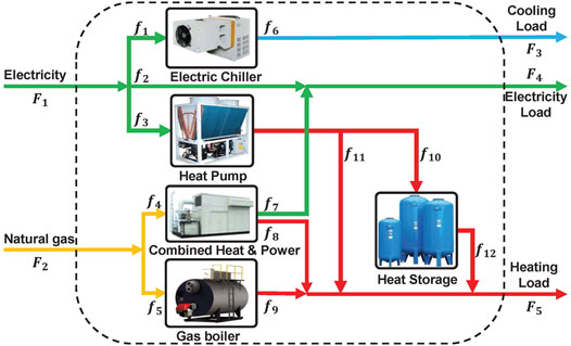
To eliminate the nonlinear problem brought by the dispatch factor, auxiliary state variables are introduced to represent each energy flow inside the EH (Wang et al., 2017b). A typical framework of EH is shown in Figure 1. The modified coupling equation of EH is given as Eq. 27.

$\left[\begin{array}{c}\hfill F_1\hfill \\ \hfill F_2\hfill \\ \hfill F_3\hfill \\ \hfill F_4\hfill \\ \hfill F_5\hfill \\ \hfill 0\hfill \\ \hfill 0\hfill \\ \hfill 0\hfill \\ \hfill 0\hfill \\ \hfill 0\hfill \\ \hfill 0\hfill \end{array}\right]=\left[\begin{array}{ccccccccccccc}\hfill 1\hfill & \hfill 1\hfill & \hfill 1\hfill & \hfill 0\hfill & \hfill 0\hfill & \hfill 0\hfill & \hfill 0\hfill & \hfill 0\hfill & \hfill 0\hfill & \hfill 0\hfill & \hfill 0\hfill & \hfill 0\hfill & \hfill 0\hfill \\ \hfill 0\hfill & \hfill 0\hfill & \hfill 0\hfill & \hfill 1\hfill & \hfill 1\hfill & \hfill 0\hfill & \hfill 0\hfill & \hfill 0\hfill & \hfill 0\hfill & \hfill 0\hfill & \hfill 0\hfill & \hfill 0\hfill & \hfill 0\hfill \\ \hfill 0\hfill & \hfill 0\hfill & \hfill 0\hfill & \hfill 0\hfill & \hfill 0\hfill & \hfill 1\hfill & \hfill 0\hfill & \hfill 0\hfill & \hfill 0\hfill & \hfill 0\hfill & \hfill 0\hfill & \hfill 0\hfill & \hfill 0\hfill \\ \hfill 0\hfill & \hfill 1\hfill & \hfill 0\hfill & \hfill 0\hfill & \hfill 0\hfill & \hfill 0\hfill & \hfill 1\hfill & \hfill 0\hfill & \hfill 0\hfill & \hfill 0\hfill & \hfill 0\hfill & \hfill 0\hfill & \hfill 0\hfill \\ \hfill 0\hfill & \hfill 0\hfill & \hfill 0\hfill & \hfill 0\hfill & \hfill 0\hfill & \hfill 0\hfill & \hfill 0\hfill & \hfill 1\hfill & \hfill 1\hfill & \hfill 0\hfill & \hfill 1\hfill & \hfill 1\hfill & \hfill 0\hfill \\ \hfill {\eta }_{\mathrm{e}\mathrm{c}}^{\mathrm{c}}\hfill & \hfill 0\hfill & \hfill 0\hfill & \hfill 0\hfill & \hfill 0\hfill & \hfill -1\hfill & \hfill 0\hfill & \hfill 0\hfill & \hfill 0\hfill & \hfill 0\hfill & \hfill 0\hfill & \hfill 0\hfill & \hfill 0\hfill \\ \hfill 0\hfill & \hfill 0\hfill & \hfill {\eta }_{\mathrm{h}\mathrm{p}}^{\mathrm{h}}\hfill & \hfill 0\hfill & \hfill 0\hfill & \hfill 0\hfill & \hfill 0\hfill & \hfill 0\hfill & \hfill 0\hfill & \hfill -1\hfill & \hfill -1\hfill & \hfill 0\hfill & \hfill 0\hfill \\ \hfill 0\hfill & \hfill 0\hfill & \hfill 0\hfill & \hfill {\eta }_{\mathrm{c}\mathrm{h}\mathrm{p}}^{\mathrm{e}}\hfill & \hfill 0\hfill & \hfill 0\hfill & \hfill -1\hfill & \hfill 0\hfill & \hfill 0\hfill & \hfill 0\hfill & \hfill 0\hfill & \hfill 0\hfill & \hfill 0\hfill \\ \hfill 0\hfill & \hfill 0\hfill & \hfill 0\hfill & \hfill {\eta }_{\mathrm{c}\mathrm{h}\mathrm{p}}^{\mathrm{h}}\hfill & \hfill 0\hfill & \hfill 0\hfill & \hfill 0\hfill & \hfill -1\hfill & \hfill 0\hfill & \hfill 0\hfill & \hfill 0\hfill & \hfill 0\hfill & \hfill 0\hfill \\ \hfill 0\hfill & \hfill 0\hfill & \hfill 0\hfill & \hfill 0\hfill & \hfill {\eta }_{\mathrm{g}\mathrm{b}}^{\mathrm{h}}\hfill & \hfill 0\hfill & \hfill 0\hfill & \hfill 0\hfill & \hfill -1\hfill & \hfill 0\hfill & \hfill 0\hfill & \hfill 0\hfill & \hfill 0\hfill \\ \hfill 0\hfill & \hfill 0\hfill & \hfill 0\hfill & \hfill 0\hfill & \hfill 0\hfill & \hfill 0\hfill & \hfill 0\hfill & \hfill 0\hfill & \hfill 0\hfill & \hfill {\eta }_{\mathrm{h}\mathrm{s}}^{\mathrm{c}\mathrm{h}\mathrm{a}\mathrm{r}}\hfill & \hfill 0\hfill & \hfill \frac{-1}{{\eta }_{\mathrm{h}\mathrm{s}}^{\mathrm{d}\mathrm{i}\mathrm{s}}}\hfill & \hfill -1\hfill \end{array}\right]\ast \left[\begin{array}{c}\hfill f_1\hfill \\ \hfill f_2\hfill \\ \hfill f_3\hfill \\ \hfill f_4\hfill \\ \hfill f_5\hfill \\ \hfill f_6\hfill \\ \hfill f_7\hfill \\ \hfill f_8\hfill \\ \hfill f_9\hfill \\ \hfill f_{10}\hfill \\ \hfill f_{11}\hfill \\ \hfill f_{12}\hfill \\ \hfill \mathrm{\Delta }E\hfill \end{array}\right](27)$

where F₁ to F₅ and f₁ to f₁₂ are the outer and inner energy flows (kW h) of the EH; ΔE is the stored energy (kW h) in the heat storage (HS) tank; ${\eta }_{\mathrm{e}\mathrm{c}}^{\mathrm{c}}$, ${\eta }_{\mathrm{h}\mathrm{p}}^{\mathrm{h}}$, ${\eta }_{\mathrm{c}\mathrm{h}\mathrm{p}}^{\mathrm{e}}$, ${\eta }_{\mathrm{c}\mathrm{h}\mathrm{p}}^{\mathrm{h}}$, ${\eta }_{\mathrm{g}\mathrm{b}}^{\mathrm{h}}$, ${\eta }_{\mathrm{h}\mathrm{s}}^{\mathrm{c}\mathrm{h}\mathrm{a}\mathrm{r}}$, ${\eta }_{\mathrm{h}\mathrm{s}}^{\mathrm{d}\mathrm{i}\mathrm{s}}$ are the energy conversion efficiencies of electric chiller (EC), heat pump (HP), combined heat and power (CHP) unit (electrical output), CHP unit (heat output), gas boiler (GB), HS (charging) and HS (discharging), respectively. Through this modification, the connection and conversion relationships are integrated into one coupling matrix, which provides considerable flexibility and simplicity to the modeling process without introducing more elements like energy buses and virtual nodes into the modeling process (Liu et al., 2020).

FIGURE 1

FIGURE 1. Framework of single EH.

2.5 Objective Function and Problem Formulation

In the system of networked EHs, the heat power of district heat network is supplied by EHs, while EHs are powered by electricity and gas from the upper networks. The objective function can be described as Eq. (28).

$C_{\mathrm{o}\mathrm{p}}=\sum _{t=1}^{N_{\mathrm{t}}}\left(P_{\mathrm{i}\mathrm{n}}{C}_{\mathrm{i}\mathrm{n}}-P_{\mathrm{o}\mathrm{u}\mathrm{t}}{C}_{\mathrm{o}\mathrm{u}\mathrm{t}}+M_{\mathrm{g}\mathrm{a}\mathrm{s}}{C}_{\mathrm{g}\mathrm{a}\mathrm{s}}\right)(28)$

where t is the index of hour; C_op is the total cost (¥) of the whole system during 24 h; N_t denotes the total scheduling time periods, which is set as 24 in this study; P_in, P_out and M_gas are the purchasing electrical power (kW h), selling electrical power (kW h) and gas flow (kcf) at gas source; C_in, C_out and C_gas are the corresponding prices (¥/kW h, ¥/kcf) for P_in, P_out and M_gas.

$Objectivefunction:\left(28\right),s.t.\left(1\right)-\left(27\right)(29)$

The formulated problem is a complicated mixed integer nonlinear programming (MINLP) problem, which can hardly be solved by existing commercial solvers. Therefore, a modified PWL method is proposed in the next section to transform part of the MINLP model (one-dimensional nonlinear functions) into the MILP formulation, which can reduce the computation difficulty.

3 Linearization Methodology

3.1 Modified Piecewise Linearization Method

In this section, a modified PWL method is proposed, with improved performance of accuracy and computation efficiency (verified in the last subsection) among popular PWL tactics, such as Taylor’s expansion based approximation (TEBA) method (Zhang et al., 2015a; Shao et al., 2016), Special Order of Sets (SOS) method (Liu et al., 2020) and binary method (Huang et al., 2020b). The proposed PWL method is based on the binary method with horizontal and vertical modifications, which are introduced in the following subsections.

3.1.1 Binary PWL Method

Through the PWL approximation, the general form of one-dimensional nonlinear function F(X) can be reformulated into the linearized function L(X). The equations of its independent variable, dependent variable, and segment range are described as Eqs 30, 31, and 32, respectively.

$X=X_0+\sum _{k=1}^N{\sigma }_k(30)$

$L\left(X\right)=F\left(X_0\right)+\sum _{k=1}^N{K}_k{\sigma }_k(31)$

$Z_{k+1}\cdot \left(\overline{X_k}-\underline{X_k}\right)\le {\sigma }_k\le Z_k\cdot \left(\overline{X_k}-\underline{X_k}\right)(32)$

where k is the index of segment; N is the total number of segments X is a continuous variable; X₀ is the minimum of X; σ_k is the value of the kth segment of X; K_k is the coefficient of the kth segment of L(X); Z_k and Z_k+1 are binary variables to guarantee the continuity of X and L(X); $\overline{X_k}$ and $\underline{X_k}$ are the upper and lower limit of the kth segment of X.

3.1.2 Horizontal Modification

The accuracy of the PWL approximation depends greatly on the selection of breakpoints. The precision of the approximation can be further improved by adding more piecewise segments. However, the addition of segments leads to a substantial increase in the computational burden. Therefore, the strategy of breakpoint selection is modified here, from the evenly-spaced selection, to the selection at the maximum error of linear approximation. The approximation error is shown as:

$E=L\left(X\right)-F\left(X\right)(33)$

where E is the error of piecewise linearization. The initial breakpoint is determined when the maximum error occurs at ∂E/∂X = 0. The following breakpoints are ranked and selected sequentially according to the maximum errors of their own ranges, as illustrated in Figure 2. This process is conducted iteratively until the maximum piecewise segment is reached or the approximation error is less than the predefined tolerance.

FIGURE 2

FIGURE 2. Horizontal Modification for PWL method.

3.1.3 Vertical Modification

Based on approximation error value, a vertical modification has been implemented on the PWL approximation, which is denoted in Eq. 34.

$L^{\prime }\left(X\right)=L\left(X\right)-\frac{{\sum }_{k=1}^N{\int }_{x_{k-1}}^{x_k}\left(L\left(X\right)-F\left(X\right)\right)dX}{{\sum }_{k=1}^N{\sigma }_k}(34)$

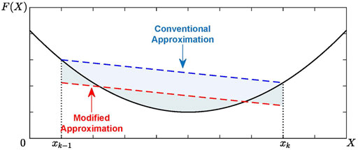
where L′(X) is the modified formulation of L(X) after vertical modification; x_k−1 and x_k are the (k−1)th and kth breakpoint for L(X). This modification can further reduce the approximation error, with its demonstration shown in Figure 3.

FIGURE 3

FIGURE 3. Vertical Modification for PWL method.

3.2 Linearization of Nonlinear Constraints

In this subsection, the above-mentioned modified PWL approach Eqs (30)–(34) will be implemented on one-dimensional nonlinear functions.

3.2.1 Modified Model for Gaseous Constraints

Variable substitutions of ${\theta }_m={\pi }_m^2,{\theta }_n={\pi }_n^2,{\phi }_{mn}={\theta }_m-{\theta }_n$ are performed to replace the original gas flow function Eq. 7 by Eq. 35. In this way, a dimension reduction is applied to the nonlinear function, which simplifies the linearization process.

$F_{\mathrm{p},mn}=\mathrm{sgn}\left({\phi }_{mn}\right)C_{mn}\sqrt{\left|{\phi }_{mn}\right|}(35)$

Besides, the substitution is applied to the variable constraints, which converts Eq. 8 into Eq. 36.

${\left({\pi }_m^{\min }\right)}^2-{\left({\pi }_n^{\max }\right)}^2\le {\phi }_{mn}\le {\left({\pi }_m^{\max }\right)}^2-{\left({\pi }_n^{\min }\right)}^2(36)$

The pressure drop equation is finally reformulated as

${\phi }_{mn}=\mathrm{sgn}\left(F_{\mathrm{p},mn}\right)\frac{{F_{\mathrm{p},mn}}^2}{{C_{mn}}^2}(37)$

The modified PWL method is then carried out on Eq. 37.

3.2.2 Modified Model for Hydraulic Constraints

The hydraulic models, including the equations of pipelines’ thermal resistance, friction factor, diameter, Reynolds number, and flow velocity, are given as Eq. 38, 39, 40, and 41, respectively.

$K_{pq}=\frac{8L_{pq}{f}_{pq}}{{D_{pq}}^5{\rho }^2{\pi }^{2}g}(38)$

$f_{pq}=\frac{0.3164}{{{Re}_{pq}}^{0.25}}(39)$

$R{e}_{pq}=\frac{v_{pq}{D}_{pq}}{\mu }(40)$

$v_{pq}=\frac{m_{\mathrm{l}\mathrm{i}\mathrm{n}\mathrm{e},pq}}{\rho \pi D_{pq}^2/4}(41)$

where K_pq, f_pq, D_pq, Re_pq and v_pq are the resistance coefficient, friction factor, diameter (m), Reynolds number and flow velocity (m/s) of pipeline pq; ρ is water density (kg/m³); g is the acceleration of gravity (kg⋅m/s²); μ is the kinematic viscosity of water (m²/s). Eq. 42 is derived from substituting Eqs. 38–41 into Eq. (18), where W denotes vector of comprehensive coefficients.

$\mathit{B}\mathit{W}{\mathit{m}}_{\mathrm{l}\mathrm{i}\mathrm{n}\mathrm{e}}|{\mathit{m}}_{\mathrm{l}\mathrm{i}\mathrm{n}\mathrm{e}}{|}^{3/4}=0(42)$

The nonlinear term in Eq. 42 can be linearized by the proposed PWL approach.

3.2.3 Modified Model for Energy Hubs

The capacities and conversion characteristics of the devices in the EH depicted in Figure 1 are shown in Table 1 (Huang et al., 2020b). The modified PWL method is applied to the nonlinear curve of each device.

TABLE 1

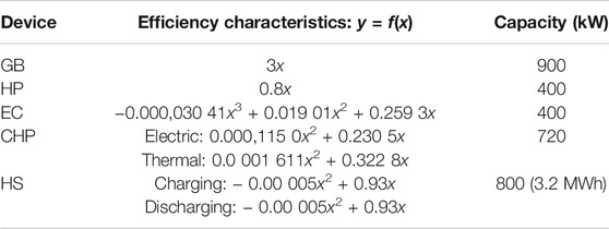
TABLE 1. Parameters for devices in Figure 1.

4 Iterative Linearization Based on SLP Algorithm

After the previous PWL section, the remaining multi-dimensional nonlinear functions are handled with the SLP algorithm in this section. The SLP obtains a feasible solution from linearized models and fixes the linearization-related inaccuracies by repeating the steps successively, leading the approximation to reach the solution (Nocedal and Wright, 2006).

4.1 Framework of Linearization and Iteration Process

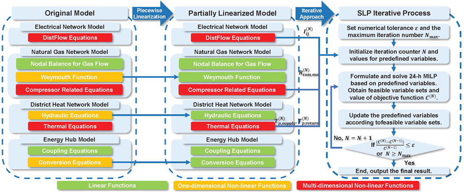
The framework of the linearization process and iteration approach is illustrated in Figure 4. In this framework, the original MINLP model is partially linearized by the proposed PWL method, and the remaining nonlinear functions are going through the iterative linearization process. Several decision variables are predefined to linearize these functions. The variables include the current term I_ij in Eqs 1–5, the compressor ratio term R_com,mn in Eqs 13, 14 and the nodal temperature terms T_p,supply, T_p,return in Eqs 21–26. The decision variables are updated through each iteration, making sure that the error caused by approximation is reduced sequentially. In this way, the model is totally linearized and forms a computational affordable MILP problem.

FIGURE 4

FIGURE 4. Framework of the linearization process and iteration approach.

4.2 Selection of Decision Variables

4.2.1 Decision Variable in Electrical Constraints

As shown in the nonlinear electrical Equation 4, the quadratic terms $P_{ij}^2$ and $Q_{ij}^2$ bring multi-dimensional nonlinearity into this formulation, which make the model difficult to be linearized. To solve this problem, Equation 4 is defined as an auxiliary constraint, which does not participate in the optimization directly but is used to update the value of I_ij repeatedly in the iteration process. Through this way, the term I_ij in Eqs 1–3 are set as constant, and thus these equations are converted into linear formulations.

4.2.2 Decision Variable in Gaseous Constraints

The three-dimensional nonlinear function Eq. 12 is difficult to linearize efficiently. In some works, the gas compressor’s consumption is replaced by an empirical ratio multiplied with the passing gas flow (Li et al., 2018). To avoid both inaccurate approximation and inefficient linearization, a hybrid method is adopted to calculate the consumption. Firstly, Equation 13 is defined as an auxiliary constraint, determining the value of compression ratio $\frac{{\pi }_n}{{\pi }_m}$ by iterative process, which transform Equation 12 into a one-dimensional function. Then, the proposed PWL method is applied to this function to remove the nonlinearity of the quadratic term.

4.2.3 Decision Variable in Hydraulic-Thermal Constraints

It is obvious that the thermal Equations 21–24 contain variable multiplications and exponential term, which introduce nonlinearity and make the hydraulic-thermal model difficult to solve. Also, common NLP and MINLP solvers met convergence problems when trying to optimize this integrated model. Therefore, Eqs 22–24 are treated as auxiliary constraints, and the nodal temperature values T_p,supply and T_p,return are determined according to the feasible solution of each iteration. In this way, the hydraulic-thermal model is transformed into a MILP format that supports rapid iteration.

4.3 Iteration Procedure

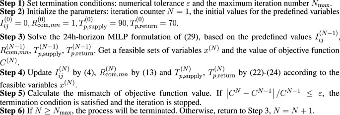
After the previous linearization process, Eq. 29 is reformulated into MILP form. An iterative approach based on SLP algorithm is carried out to get the final solution. The specific details are provided in Algorithm 1.

ALGORITHM 1

Algorithm 1. Iterative Algorithm Based on Sequential Linear Programming.

5 Case Studies

5.1 Accuracy and Efficiency Verification for the Proposed PWL Method

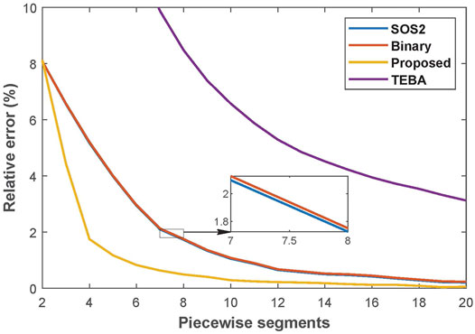
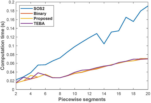
This subsection tests the performance of three mainstream PWL methods and the proposed PWL method in an optimization problem. The three PWL methods include Taylor’s expansion based Approximation (TEBA) method (Zhang et al., 2015a; Shao et al., 2016), Special Order of Sets 2 (SOS2) method (Liu et al., 2020), and Binary method (Huang et al., 2020b). The optimization problem is formulated as the day-ahead optimal scheduling of single EH shown in Figure 1. The EH contains two devices with linear efficiency curves and three devices with nonlinear efficiency curves, shown in Table 1. The optimization result is illustrated and compared in Figures 5 and 6.

FIGURE 5

FIGURE 5. Relative errors of four PWL approaches with increasing segments.

FIGURE 6

FIGURE 6. Computation time of four PWL approaches with increasing segments.

It is worth noting that when the number of piecewise segments gets large enough, all the methods obtain a relatively precise approximation. However, a large number of segments is impractical since the number of extra binary variables and constraints has a considerable impact on computational efficiency. Therefore, in this comparison, the maximum segment is limited to 20. The benchmark values are derived from directly solving the nonlinear problem by the nonlinear programming (NLP) solver IPOPT.

Figures 5 6 compare the approximation accuracy and computation efficiency of these four methods. The results come from the average of 100 calculations. As shown in Figure 5, the proposed method’s error drops fastest as the number of segments increases. In this case, the proposed method, Binary method, SOS2, and TEBA, require 5, 10, 10, and more than 20 segments, respectively, to achieve an error of less than 1%. It suggests that, given the same number of segments, the proposed method’s accuracy is clearly superior to other methods. As can be seen from Figure 6, the calculation time of the proposed method, Binary method and TEBA is nearly the same with the increasing segment number, while SOS2 requires a larger computation time. Since the proposed method can reduce the calculation error to an acceptable level with fewer segments, its accuracy advantage can be converted into a boost in computational efficiency.

5.2 Evaluation of Simulation Result

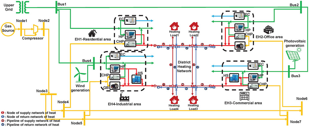
In this subsection, the numerical solution of the optimal scheduling problem is analyzed to confirm the effectiveness of proposed approach of iterative linearization. The demonstration system in Figure 7 is composed of 4-bus electrical system, 7-node natural gas network, 8-node district heating network (with looped configuration of supply and return pipelines) and four EHs representing different regional IESs, including residential area, commercial area, industrial area and office area with specific layout of equipment and load characteristics.

FIGURE 7

FIGURE 7. Schematic of the system composed of four networked EHs.

A set of cases are designed and tested to evaluate the performance of the proposed method. Due to the heavy nonlinearity, the original MINLP model in Eq. 29 is not solvable for the mainstream solvers like FMINCON and IPOPT (By replacing the binary variables bin with constraint bin (1 − bin) = 0, the MINLP problem can be transformed into NLP formulation, which expands the choices of solvers) (Yang et al., 2020). Thus, the solution of the proposed method with high numbers of iterations and piecewise segments is considered accurate and taken as the reference value to compare with other results. Simulation results are obtained from a PC with an Intel Core of i5-7400U 3.00GHz CPU and 16GB RAM; the YALMIP toolbox (Lofberg, 2004) has been used to develop the optimization programs in Matlab R2019a; the solver for nonlinear programming is IPOPT and the MILP problems are solved by GUROBI.

• Case 1: The proposed method is carried out with the convergence tolerance of 10⁻⁵ and the piecewise segment of 30. The result is regarded as the benchmark value for further comparison.

• Case 2: The MINLP model in Eq. 29 is implemented and solved. To make sure that the original nonlinear model is solvable, the conversion efficiencies for devices of EHs are set as constants and the constraints of the heat network are simplified according to (Shabanpour-Haghighi and Seifi, 2015a).

• Case 3: The proposed method is performed with the convergence tolerance of 10⁻³ and the piecewise segment of 10.

Table 2 presents a comparison of optimization results for three different cases. The table shows that the calculation time and relative error of Case 3 are significantly less than those of Case 2, demonstrating the proposed method’s improved accuracy and computation efficiency.

TABLE 2

TABLE 2. Optimization result comparison for different cases.

In terms of the calculation time, Case 3 has a clear advantage due to its fast computation (due to its MILP formulation) and fewer iterations. Case 2 is slow due to its MINLP property. In terms of the relative error, Case 3 has good performance since the modified PWL method and iterative approach fix the approximation deviation. Case 2 has a high relative error of 11.694%, mainly because its model is not accurate enough. The electrical and gaseous models are considered accurate because the original nonlinear constraints are taken. The inaccuracy is mainly introduced by simplifying the heating model (neglecting hydraulic constraints and return pipelines) and constant conversion efficiencies adopted for EHs.

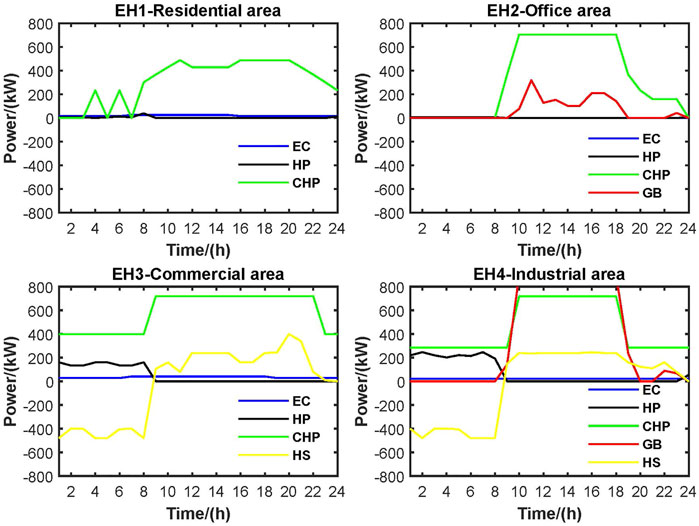
Figure 8 shows the operating states of 4 EHs, obtained from the optimization result of Case 3. It is worth noting that the CHP unit in each region is given the highest priority for operation due to its good economic performance. The HS plays a vital role in EH3 and EH4, especially when cooperating with HP. The HP generates heat and stores it in the HS during the peak time of electricity, then the HS release heat during the off-peak time of electricity. However, the HPs are not active in EH1 and EH2 due to the absence of HS. In EH4, the GB is heavily used during the day, while the HP is active at night, since gas is relatively cheaper than electricity in daylight hours.

FIGURE 8

FIGURE 8. Operation states of energy converters of four regional EHs.

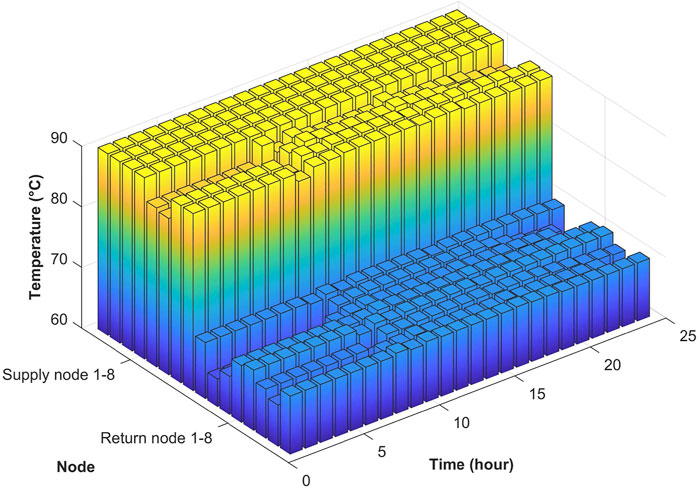
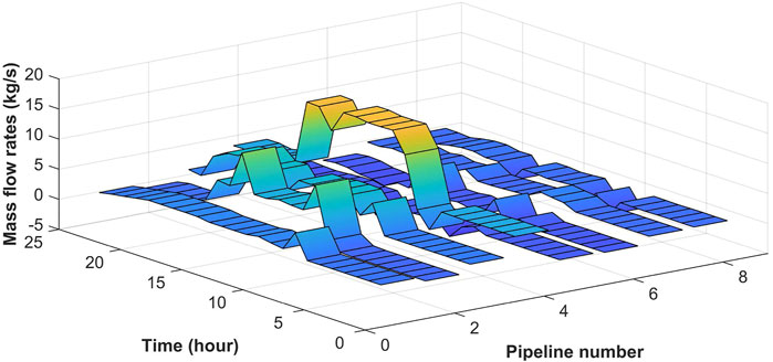
Since the VF-VT model of heat network is adopted, the mass flow of each pipe and the temperature of each node can be obtained in the optimization, as illustrated in Figures 9 and 10.

FIGURE 9

FIGURE 9. Temperatures for each node in the heat network.

FIGURE 10

FIGURE 10. Mass flow rate for each pipe in the heat network.

Unlike the CF-VT mode, which is extensively utilized in China, Russia, and part of Northern European countries, the VF-VT mode can more flexibly manage the flow and thus alter the total quantity of heat given to each node. In the study case, the heat loads in regions one to four are mostly concentrated throughout the daytime, and the peak load of the industrial zone is significantly higher than that of other regions, posing significant challenges to IES collaborative scheduling. As demonstrated in Figure 10, each pipeline can vary its flow dramatically with the VF mode to meet a load curve that fluctuates greatly throughout the day. Among all the pipelines, pipeline 4 has the highest flow and changes the most during the day since it is mostly utilized to supply the heat load in the industrial area.

5.3 Adaptability Analysis

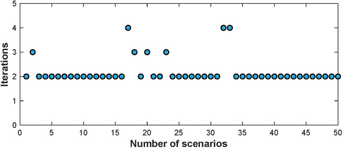
Assume that loads of electricity, heat, and gas differ uniformly with a proportion of 10% compared to the initial load values. The Monte Carlo simulation method is adopted to produce 50 scenarios with fluctuating loading conditions.

Figure 11 demonstrates the variations of the solutions under multiple scenarios. It is demonstrated that most scenarios converge within two iterations. Only a few of them require one or two more iterations, validating the convergence and adaptability of the proposed approach.

FIGURE 11

FIGURE 11. Iterations of the proposed method in scenarios of fluctuating loads.

6 Conclusion

This paper proposes a modified piecewise linearization (PWL) method to improve the linearization performance and combines it with the sequential linear programming (SLP) algorithm to deal with the multi-dimensional nonlinear problem. The formulated mixed integer linear programming (MILP) problem is tested in a multi-regional integrated energy system (MIES) including electrical, heat, and gas networks as well as four energy hubs (EH) representing residential, commercial, industrial, and office regions, respectively. The results demonstrate that the iterative linearization method can solve the optimal scheduling problem of a multi-region integrated energy system accurately and efficiently while keeping a modest number of segments and iterations. In addition, the findings from this study make several contributions to the current literature:

1. The method presented in this paper helps solve two kinds of problems that are difficult to deal with by traditional PWL methods. The first problem is the slowdown in computation speed caused by the introduction of integer variables. In this study, the PWL method is improved to accomplish the same effect with fewer segments, minimizing the calculation time increased by the additional integer variables. The other problem is that dealing with multivariable nonlinear equations is challenging using the traditional PWL method. In this work, the PWL method is combined with the SLP algorithm to transform a complex mixed integer nonlinear programming (MINLP) problem into a MILP problem that can be solved efficiently with the powerful state-of-the-art MILP solvers.

2. The proposed method can achieve a more desirable trade-off between accuracy and computational efficiency when solving MILP problems, which is especially suitable for complex and nonlinear multi-regional integrated energy system scheduling problems. Compared with the original nonlinear model, the newly formulated MILP model is computationally cheaper with only a slight loss in accuracy. The results of the case study show that the two factors that may slow down the computational efficiency, namely segments and iterations, can be kept within a tolerable range and hence have a minimal effect on calculation performance.

Although the proposed algorithm has successfully demonstrated its effectiveness in solving MINLP problems, it lacks certain considerations in terms of time-scale interaction mechanisms between multiple energy systems, as well as the time delay and energy storage effect of gas/heating pipelines. Taking these considerations into account, the proposed algorithm has not been proven to be effective, which means it will be investigated further in our future work.

Data Availability Statement

The original contributions presented in the study are included in the article/Supplementary Material, further inquiries can be directed to the corresponding author.

Author Contributions

HT: Conceptualization, Methodology, Software, Validation, Formal analysis, Investigation, Writing-original draft, Visualization, Resources. HZ: Methodology, Software, Validation, Writing-review editing, Supervision, Project administration, Funding acquisition. CL: Methodology, Validation, Writing-review editing, Project administration. JC: Methodology, Writing-review editing, Project administration.

Funding

This work was supported by National Key R&D Program of China under grant 2018YFA0702200.

Conflict of Interest

The authors declare that the research was conducted in the absence of any commercial or financial relationships that could be construed as a potential conflict of interest.

Publisher’s Note

All claims expressed in this article are solely those of the authors and do not necessarily represent those of their affiliated organizations, or those of the publisher, the editors and the reviewers. Any product that may be evaluated in this article, or claim that may be made by its manufacturer, is not guaranteed or endorsed by the publisher.

References

Bao, Y.-Q., Wu, M., Zhou, X., and Tang, X. (2019). Piecewise Linear Approximation of Gas Flow Function for the Optimization of Integrated Electricity and Natural Gas System. IEEE access 7, 91819–91826. doi:10.1109/ACCESS.2019.2927103

CrossRef Full Text | Google Scholar

Geidl, M., and Andersson, G. (2005). “A Modeling and Optimization Approach for Multiple Energy Carrier Power Flow,” in 2005 IEEE Russia Power Tech (IEEE), 1–7. doi:10.1109/PTC.2005.4524640

CrossRef Full Text | Google Scholar

He, Y., Shahidehpour, M., Li, Z., Guo, C., and Zhu, B. (2018). Robust Constrained Operation of Integrated Electricity-Natural Gas System Considering Distributed Natural Gas Storage. IEEE Trans. Sustain. Energ. 9, 1061–1071. doi:10.1109/TSTE.2017.2764004

CrossRef Full Text | Google Scholar

Huang, W., Zhang, N., Cheng, Y., Yang, J., Wang, Y., and Kang, C. (2020a). Multienergy Networks Analytics: Standardized Modeling, Optimization, and Low Carbon Analysis. Proc. IEEE 108, 1411–1436. doi:10.1109/JPROC.2020.2993787

CrossRef Full Text | Google Scholar

Huang, W., Zhang, N., Wang, Y., Capuder, T., Kuzle, I., and Kang, C. (2020b). Matrix Modeling of Energy Hub with Variable Energy Efficiencies. Int. J. Electr. Power Energ. Syst. 119, 105876. doi:10.1016/j.ijepes.2020.105876

CrossRef Full Text | Google Scholar

Li, Y., Li, Z., Wen, F., and Shahidehpour, M. (2019). Privacy-preserving Optimal Dispatch for an Integrated Power Distribution and Natural Gas System in Networked Energy Hubs. IEEE Trans. Sustain. Energ. 10, 2028–2038. doi:10.1109/TSTE.2018.2877586

CrossRef Full Text | Google Scholar

Liu, B., Meng, K., Dong, Z. Y., and Wei, W. (2019). Optimal Dispatch of Coupled Electricity and Heat System with Independent thermal Energy Storage. IEEE Trans. Power Syst. 34, 3250–3263. doi:10.1109/TPWRS.2019.2901254

CrossRef Full Text | Google Scholar

Liu, F., Bie, Z., and Wang, X. (2019). Day-ahead Dispatch of Integrated Electricity and Natural Gas System Considering reserve Scheduling and Renewable Uncertainties. IEEE Trans. Sustain. Energ. 10, 646–658. doi:10.1109/TSTE.2018.2843121

CrossRef Full Text | Google Scholar

Liu, T., Zhang, D., and Wu, T. (2020). Standardised Modelling and Optimisation of a System of Interconnected Energy Hubs Considering Multiple Energies-Electricity, Gas, Heating, and Cooling. Energ. Convers. Manag. 205, 112410. doi:10.1016/j.enconman.2019.112410

CrossRef Full Text | Google Scholar

Liu, X., Wu, J., Jenkins, N., and Bagdanavicius, A. (2016). Combined Analysis of Electricity and Heat Networks. Appl. Energ. 162, 1238–1250. doi:10.1016/j.egypro.2014.11.92810.1016/j.apenergy.2015.01.102

CrossRef Full Text | Google Scholar

Lofberg, J. (2004). “Yalmip: A Toolbox for Modeling and Optimization in Matlab,” in 2004 IEEE international conference on robotics and automation (IEEE Cat. No. 04CH37508) (IEEE), 284–289.

Google Scholar

Low, S. H. (2014). Convex Relaxation of Optimal Power Flow-Part I: Formulations and Equivalence. IEEE Trans. Control. Netw. Syst. 1, 15–27. doi:10.1109/TCNS.2014.2309732

CrossRef Full Text | Google Scholar

Mancarella, P. (2014). Mes (Multi-energy Systems): An Overview of Concepts and Evaluation Models. Energy 65, 1–17. doi:10.1016/j.energy.2013.10.041

CrossRef Full Text | Google Scholar

Manshadi, S. D., and Khodayar, M. E. (2018b). A Tight Convex Relaxation for the Natural Gas Operation Problem. IEEE Trans. Smart Grid 9, 5467–5469. doi:10.1109/TSG.2018.2817069

CrossRef Full Text | Google Scholar

Manshadi, S., and Khodayar, M. (2020a). Coordinated Operation of Electricity and Natural Gas Systems: A Convex Relaxation Approach. IEEE Trans. Smart Grid 10, 3342–3354. doi:10.1109/PESGM41954.2020.9281784

CrossRef Full Text | Google Scholar

Moeini-Aghtaie, M., Abbaspour, A., Fotuhi-Firuzabad, M., and Hajipour, E. (2014). A Decomposed Solution to Multiple-Energy Carriers Optimal Power Flow. IEEE Trans. Power Syst. 29, 707–716. doi:10.1109/TPWRS.2013.2283259

CrossRef Full Text | Google Scholar

Molzahn, D. K., Dörfler, F., Sandberg, H., Low, S. H., Chakrabarti, S., Baldick, R., et al. (2017). A Survey of Distributed Optimization and Control Algorithms for Electric Power Systems. IEEE Trans. Smart Grid 8, 2941–2962. doi:10.1109/TSG.2017.2720471

CrossRef Full Text | Google Scholar

Nocedal, J., and Wright, S. (2006). Numerical Optimization. Springer Science & Business Media.

Google Scholar

Shabanpour-Haghighi, A., and Seifi, A. R. (2015a). Energy Flow Optimization in Multicarrier Systems. IEEE Trans. Ind. Inf. 11, 1067–1077. doi:10.1109/TII.2015.2462316

CrossRef Full Text | Google Scholar

Shabanpour-Haghighi, A., and Seifi, A. R. (2015b). Multi-objective Operation Management of a Multi-Carrier Energy System. Energy 88, 430–442. doi:10.1016/j.energy.2015.05.063

CrossRef Full Text | Google Scholar

Shao, C., Ding, Y., Wang, J., and Song, Y. (2018). Modeling and Integration of Flexible Demand in Heat and Electricity Integrated Energy System. IEEE Trans. Sustain. Energ. 9, 361–370. doi:10.1109/TSTE.2017.2731786

CrossRef Full Text | Google Scholar

Shao, C., Wang, X., Shahidehpour, M., Wang, X., and Wang, B. (2017). An Milp-Based Optimal Power Flow in Multicarrier Energy Systems. IEEE Trans. Sustain. Energ. 8, 239–248. doi:10.1109/TSTE.2016.2595486

CrossRef Full Text | Google Scholar

Sheikhi, A., Bahrami, S., and Ranjbar, A. M. (2015). An Autonomous Demand Response Program for Electricity and Natural Gas Networks in Smart Energy Hubs. Energy 89, 490–499. doi:10.1016/j.energy.2015.05.109

CrossRef Full Text | Google Scholar

Wang, C., Wei, W., Wang, J., Bai, L., Liang, Y., and Bi, T. (2018a). Convex Optimization Based Distributed Optimal Gas-Power Flow Calculation. IEEE Trans. Sustain. Energ. 9, 1145–1156. doi:10.1109/TSTE.2017.2771954

CrossRef Full Text | Google Scholar

Wang, Y., Zhang, N., Kang, C., Kirschen, D. S., Yang, J., and Xia, Q. (2019b). Standardized Matrix Modeling of Multiple Energy Systems. IEEE Trans. Smart Grid 10, 257–270. doi:10.1109/TSG.2017.2737662

CrossRef Full Text | Google Scholar

Yang, L., Zhao, X., and Xu, Y. (2020). A Convex Optimization and Iterative Solution Based Method for Optimal Power-Gas Flow Considering Power and Gas Losses. Int. J. Electr. Power Energ. Syst. 121, 106023. doi:10.1016/j.ijepes.2020.106023

CrossRef Full Text | Google Scholar

Zhang, X., Shahidehpour, M., Alabdulwahab, A., and Abusorrah, A. (2016a). Hourly Electricity Demand Response in the Stochastic Day-Ahead Scheduling of Coordinated Electricity and Natural Gas Networks. IEEE Trans. Power Syst. 31, 592–601. doi:10.1109/TPWRS.2015.2390632

CrossRef Full Text | Google Scholar

Zhang, X., Shahidehpour, M., Alabdulwahab, A., and Abusorrah, A. (2015b). Optimal Expansion Planning of Energy Hub with Multiple Energy Infrastructures. IEEE Trans. Smart Grid 6, 2302–2311. doi:10.1109/TSG.2015.2390640

CrossRef Full Text | Google Scholar