 Shengxin Sun
 Chenyu Tang
 Gulizhati Hailati
 Da Xie
- 1The Key Laboratory of Control of Power Transmission and Conversion, Ministry of Education, The Department of Electrical Engineering, Shanghai Jiao Tong University, Shanghai, China
- 2The Department of Automation, The School of Intelligent Manufacturing and Control Engineering, Shanghai Polytechnic University, Shanghai, China
Due to the low inertia of the DC microgrid, the DC bus voltage is prone to drop or oscillate under disturbance. It is also challenging to supervise the stability of a DC microgrid since it is a highly nonlinear dynamic system with high dimensionality and randomness. To tackle this problem, this paper proposes a new method using ANN-aided nonlinear dynamic stability analysis for monitoring the DC bus voltage, which is combined with two steps. The first step is to establish six corresponding nonlinear accurate discrete iterative models of six switching modes of the PV-battery-load-based DC microgrid system, based on the Poincaré map theory, in order to judge the stability quantitatively with a promoted stability margin index. The second step is to use artificial neural networks (ANNs) to forecast the operating mode of the system when random changes occur in environmental circumstances and load power; this will aid the first step in being efficient and adaptable while determining stability cases. And the employed ANNs are trained with the datasets, including the circuit data, ambient temperature, irradiance, and load power, which are generated by MATLAB/Simulink simulation. Theoretical and simulation analyses are carried out under different operating conditions to validate the proposed method’s efficacy in judging the DC microgrid’s destabilizing oscillation and stable running.
1 Introduction
The DC microgrid emerged due to the integration of DC distributed energy resources (DERs), installation of battery storage systems (BSSs) and growing use of DC loads (Ahmed et al., 2020). In addition, there has been a recent increase in research interest in it, mostly because of its high transmission efficiency and good quality, requiring few power conversion stages and no reactive power (Zolfaghari et al., 2022). However, the DC microgrid utilizes numerous power electronic devices to interface energy sources and consumers, resulting in low inertia, particularly when operated independently of the primary power grid (Holari et al., 2021). This is manifested in variations in the behavior of the microgrid’s interface inputs or outputs, such as random intermittent fluctuations in the DERs and rapid changes in power loads, which can result in the DC bus voltage sagging or oscillating (Lu et al., 2015; Xia et al., 2019). Furthermore, as the scale of the modern DC microgrids continues to expand, the characteristics of high-dimensionality, nonlinearity, and strong coupling have become increasingly apparent (Zia et al., 2019), posing substantial operational security changes. Therefore, it is clear that a practical stability monitor approach that enables real-time monitoring of the microgrid’s status and provides the basis for online tuning controller parameters to achieve adequate adaptive control could be valuable (Khodamoradi et al., 2019).
Stability monitoring methods for DC microgrids include linear and nonlinear analysis methods. The linear analysis method (Eberlein and Rudion, 2021) uses the averaged model of linear approximation in the neighbourhood of the equilibrium point to analyze small-signal stability. Nonetheless, the effective range of the linearization region is frequently unclear, and the DC microgrid contains distinct and complex nonlinear features that are largely ignored, causing the stability calculations to be grossly distorted. Thus, nonlinear stability analysis is more appropriate for DC microgrids.
Nonlinear stability analysis is primarily based on nonlinear models, including quadratic or cubic nonlinear models, piecewise linear models, and discrete iterative models. According to the Taylor expansion, quadratic or cubic nonlinear models (Wang et al., 2018) retain partial nonlinear high-order terms at the equilibrium point. Piecewise linear models (Marx et al., 2012) are formed of a finite number of local linear models to approximate the original nonlinear model. Discrete iterative models (Aroudi et al., 2007) are characterized by a finite number of dynamical models corresponding to a set of toggling switching conditions. This is based on the Poincaré map theory of nonlinear dynamics, which is suitable for discontinuous systems in control engineering, such as power electronic circuits. As for a single converter system, the models above can accurately reflect the nonlinear characteristics to varying degrees. Researchers have developed various stability analysis methods such as the numerical simulation method (Seth and Banerjee, 2020), Lyapunov direct method (Toro et al., 2021), Takagi-Sugeno method (Mehran et al., 2009), saltation matrix (Wu et al., 2020), trajectory sensitivities (Geng and Hiskens, 2019), and Jacobian matrix eigenvalue analysis (Wang et al., 2020). However, as the DC microgrids expand, the number of electronic power conversion devices and the systems’ scale will increase. Consequently, these approaches may encounter numerous issues, such as extensive computation, slow calculation rates, low conservative analysis results, complex subspace division, difficulty solving the saltation matrix, and difficulty deriving the Jacobian matrix.
Therefore, in light of DC microgrids with complex structures, improved stability analysis methods are proposed according to the Lyapunov theory in (Zhang et al., 2022) and (Xie et al., 2021) for various DC microgrids. However, the offered solutions are limited to specific equivalent models, challenging generalization to other systems. Moreover, References (Ahmadi and Kazemi, 2020) and (Xia et al., 2020) present a nonlinear analysis framework applicable to other DC microgrids. Nevertheless, the modeling process is cumbersome and requires manual screening of features to reduce order, which makes it difficult to achieve flexible and accurate system monitoring. To address this issue, data-driven methods utilizing artificial intelligence technology are being developed, which primarily aim to classify prediction models or fit stable regions in various scenarios. Decision trees (Vanfretti and Narasimham Arava, 2020), support vector (Gomez et al., 2011), deep learning (Tian et al., 2022), and artificial neural network (ANN) (Tan et al., 2019) are relevant techniques. In references (Gomez et al., 2011; Tan et al., 2019; Vanfretti and Narasimham Arava, 2020; Tian et al., 2022), classical stability analysis methods are combined with intelligent technologies to achieve intelligent stability monitoring via offline training and online testing using massive datasets. Existing research focuses mostly on the traditional power system, and the intelligent stability monitoring approaches to DC microgrids are relatively rare.
To monitor the performance of DC microgrids, an intelligent nonlinear stability monitoring tool is urgently required. Poincaré map is a conventional and effective stability analysis theory in nonlinear dynamics (Tse and Di Bernardo, 2002; Moreno-Font et al., 2009). However, as the number of power electronic switches in the system increases, the iterative mapping order becomes difficult to determine, which makes it challenging to construct discrete iterative models and estimate stability calculations. Consequently, driven by the intelligent background, this paper proposes a voltage monitoring method using the Poincaré map combined with an artificial neural network for the PV-battery-load-based DC microgrid. The neural network predicts the operation mode, which facilitates discrete iterative modeling and Jacobian matrix calculation under varying input and output conditions. Thus, a stability margin is provided to quantify the operational performance. A typical case study is utilized to validate conclusions.
The remainder of this paper is structured as follows: Section 2 describes the structure and discrete iterative model of the DC microgrid; Section 3 presents the ANN-aided nonlinear voltage stability monitor method; Section 4 validates the proposed approach in numerical simulations of real scenes; Section 5 reports the conclusions of this paper.
2 Structure and modeling of the DC microgrid
2.1 Structure of the DC microgrid
Figure 1 depicts the structure of the conventional PV-battery-load-based DC microgrid understudied, which comprises a PV distributed generator (PVDG), a battery storage system (BSS), and a constant power load (CPL). The PVDG is linked to the DC bus with its boost converter. And the BSS is also connected to the same DC bus through a bidirectional dc/dc converter. As to the CPL, its equivalent model (Rahimi and Emadi, 2009) is linked to the DC bus with a buck converter. The model represents a real system to some extent. A control system contains the corresponding cascaded-PI reference voltage-current control for each device, which controls corresponding switches to ensure the uninterrupted power flow. And we refer to the cascaded-PI reference voltage-current control as the PI control for short. Particularly, the PVDG side has a maximum power point tracking (MPPT) controller and a PI controller, which can ensure the PV arrays operate at the maximum power point in any weather condition. The PI controller of BSS adjusts the operational status of the bidirectional DC/DC converter to keep the BSS charge/discharge working in a predefined state of the charge band and simultaneously maintain the DC bus voltage stable. This article assumes that the battery state can always meet the working conditions. The PI controller of CPL ensures that loads of different powers can work in the corresponding rated state.
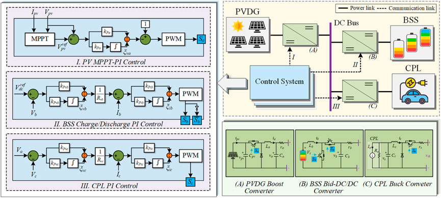
FIGURE 1. Structure of the PV-battery-load-based DC microgrid system.
2.2 Modeling of the DC microgrid
2.2.1 State equations
In nonlinear dynamics, the DC microgrid is considered a discontinuous piecewise affine system whose structure is altered when certain conditions change. The state space of the system model is divided into a finite number of non-smooth continuous subspaces, where the system model differs according to the subspace. In the power electronic switch control system, the partition of the subspace corresponds to the control law of the state change of the switch. In the following discussion, it is assumed that PVDG, BSS, and CPL remain in operation. To simplify the calculation and algorithm, the corresponding boost, buck, and bidirectional DC/DC converters of PVDG, BSS, and CPL devices are set to have the same switching frequency, and the start and end of a switching cycle are the same. Figure 2 depicts the switching timing diagrams of the three converters. Specifically, Sm =1 (m = a, b, c) presidents that the power switch is turned ON, and Sm = 0 presidents that it is turned OFF, where the subscript “m” is utilized to represent the variable associated with corresponding devices of the DC microgrid system, i.e. for the PVDC device (a), the BSS device (c), the CPL device (c). Therefore, the stable operation modes are classified into six types, including M1, M2, M3, M4, M5, M6, based on the six different switching sequences of the three switches. In Figure 2, t0, t1, t2, t3, and t4 are the switching instants when the switch is flipped. Moreover, the system structure and its corresponding state equation change 4 times when the four switch conditions toggle in turn during one period for each operation mode.
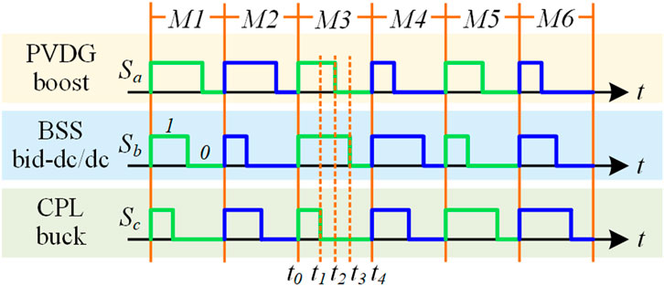
FIGURE 2. Switching sequence diagrams and six stable operation modes.
According to the four switch conditions toggling, the piecewise state equations for each operation mode in one period are as follows:
where, x = [xpv, xbss, xcpl]T is the state variable vector for the PV-battery-load-based DC microgrid system, which consists of the PVDG state vector xpv = [vpv, ia, va, ξva]T, the BSS state vector xbss = [ib, vb, ξvb, ξib]T, and the CPL state vector xcpl = [ic, vc, ξvc, ξic]T. Concretely, vpv is the output voltage of the PV arrays, im and vm (m = a, b, c) are the current of the inductance Lm and the voltage of the capacitance Cm in the corresponding converter, and ξvm and ξim are the integrated outputs of the PI voltage and current loops, respectively, as shown in Figure 1. A1, B1, A2, B2, A3, B3, A4, and B4 are state matrices, changing with the operation mode varying, and their detailed descriptions of six operation modes are given in Table 1.
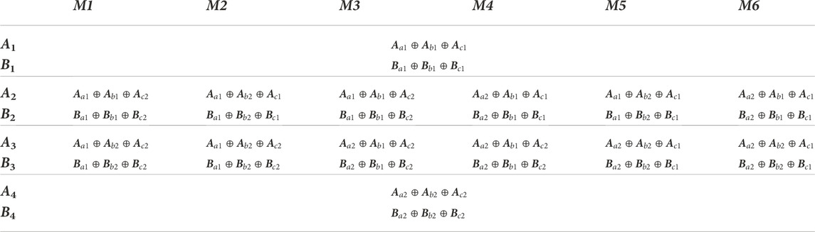
TABLE 1. State matrices of six operation modes.
In Table 1, Am1, Bm1, Am2, and Bm2 (m = a, b, c) are the state matrices for PVDG, BSS, and CPL devices. Concretely, Am1 and Bm1 correspond to the power switch on with Sm =1, and Am2 and Bm2 correspond to the power switch off with Sm = 0. And they are expressed as follows:
Where, kPvm, kIvm, kPim, kIim, Rvm (m = a, b, c) are proportional, integral, damping coefficients of corresponding PI controllers, rm is the line resistance between the equipment and the DC bus, Vs is the output voltage of the batteries, Pc and Vo are the output voltage and power at the operating point of the CPL, and V ref dc is the reference voltage of the DC bus, as shown in Figure 1.
It should be mentioned that while the matrices A1, B1, A2, B2, A3, B3, A4 and B4 are direct sums of Am1, Bm1, Am2, and Bm2, there remains still some coupling between the state equations of the individual devices linked together with the DC bus.
2.2.2 Discrete iterative model
In the nth switching cycle, let the initial conditions of state variables at the beginnings of the nth and (n+1)th switching cycle be marked as xn and xn+1. Based on the Poincaré map (Aroudi et al., 2007), during one period, local maps Pk (k = 1, 2, 3, 4) can be defined as the following forms:
where
where
The global Poincaré map P from the nth to (n+1)th switching cycle, can be defined as a composition of four different local maps Pk:
where the mathematical symbol “
Therefore, the discrete iterative map from
where
3 ANN-aided nonlinear voltage stability monitor method
3.1 Principle of nonlinear analysis
Based on the Poincaré map theory, observing the position of the eigenvalues of Jacobian matrix JP at fixed point x* in relation to the unit circle can be used to determine the nonlinear dynamic behaviour of the DC microgrid system. In addition, the eigenvalues can be determined from the eigenequation at the fixed-point x*, which consists of the following:
where λ is the eigenvalue of JP, and if all eigenvalues have a modulus length less than 1, the system is stable; otherwise, the system is unstable.
The Jacobian matrix JP is expressed as (Wang et al., 2020):
where
where xref = [
M1: K1 = 01×4
M2: K1 = 01×4
M3: K1 = 01×4
M4: K1 = Ka
M5: K1 = 01×4
M6: K1 = Ka
In combination with 5 and 7, there are:
where
Furthermore, the eigenvalue modulo length obtained from Eqn 6 can be used to reflect the system’s operating conditions and stability margins. Here, the proposed stability margin ε is defined as:
where ε represents the degree of system stability, and λMax represents the eigenvalue with the longest modulus. Define a critical value εr > 0, which is the minimum value of the system stability margin. A warning will be issued if the system stability margin drops below the critical level. And if the system is stable, 1 > ε > εr, otherwise ε < 0.
3.2 Implementation of ANN
The above content illustrates the theoretical principle of nonlinear analysis, which is dependent upon the system state. In this section, ANNs is applied to complete the procedure of multivariate classification to achieve the operating prediction mode. Figure 3A shows our neural network structure, which is fully connected and includes a 7-dimensional input layer, a 6-dimensional output layer, and four hidden layers. Specifically, the input vector [T, G, ipv, vpv, ib, ic, vdc] including ambient temperature (T), solar irradiance (G), the output current and voltage of PV arrays (ipv and vpv), the output current of battery (ib), the running current of CPL (ic), and the DC bus voltage (vdc), are the measured variables of the DC microgrid system, and the output is the probability of the operating modes P(Mi) (i = 1, 2, ...,6). Moreover, the neural node structure is illustrated in Figure 3B, which contains a linear and a nonlinear portion. The hyperparameters of the linear portion include connection weighs vector w[l,h] and a bias factor b[l,h] (l presents the serial number of the hidden layers, and h presents the serial number of neurons in one hidden layer). The nonlinear portion adopts Rectified Linea Unit (ReLU) function as an activation function f(u). The generic structure of the neural node can be stated as follows:
where r[l,h] is the input of the activation function f, y[l,h] is the output of the hth neural node in the lth hidden layer, and p presents the number of neurons in the previous layer.
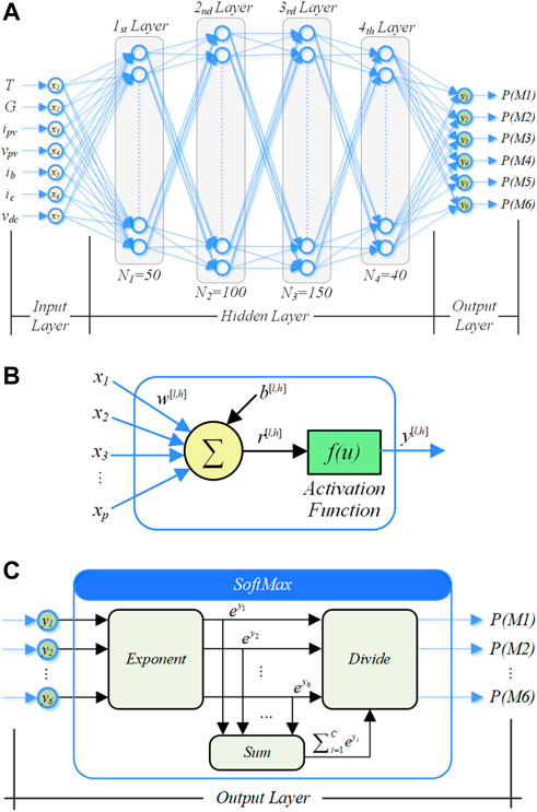
FIGURE 3. The structure of the designed ANNs. (A) The detailed structural information of the neural network. (B) The neural node structure. (C) The structure of SoftMax in the output layer.
Furthermore, the output of the full-connected ANNs is converted into the form that fulfils Formula (15) by the SoftMax algorithm, and its structure is shown in Figure 3C.
where Mi represents the operation mode, and P(Mi) is the probability of each operating state, yi is the input of the output layer, as well as the output of the full connected layers, and C = 6 represents total six operation modes, namely six outputs of the ANNs. The SoftMax algorithm is to normalize the values of the output layer lie in the range (0, 1) and the sum of the values equal 1, as expressed in Formula (16), so that these output values can be interpreted as probabilities, where the highest probability is most like the best candidate label (Maxwell et al., 2017).
Moreover, together with the Cross-Entropy Loss, SoftMax Cross-Entropy Loss is arguably one of the most commonly used in classification tasks using neural network (Liu et al., 2016). So, it is used as the loss function of the system, as follows:
where Loss is the loss function, N is the number of samples, i and j present each sample, and sji is a symbol function that can take either 0 or 1. Specifically, when the jith output value is the best candidate label, sji is 1, and others is 0.
Above all, the framework of the proposed ANN-aided nonlinear voltage stability monitor method is illustrated in Figure 4. The proposed method consists of two parts. The first step is the nonlinear stability analysis algorithm. It is based on the Poincaré map theory in nonlinear dynamics, according to the model demonstrated in Section 2.2 and the formula of calculating the stability margin ε derived in Section 3.1, to write the algorithm to evaluate the system’s stability quantitatively. In the second step, the ANNs are used to predict the operating mode of the DC microgrid. To aid the first step in efficient computation, when environmental conditions and CPL change randomly, the results predicted by the ANNs are passed on to it. To be more specific, the data set [T, G, ipv, vpv, ib, ic, vdc] generated by MATLAB/Simulink simulation is divided into training and test sets. Then the ANNs are trained and tested, and the predicted operating mode results are fed to stable calculations. We should point out that this paper calculates stability for a specific system state and does not consider the changing process between the two states.
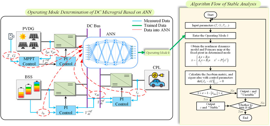
FIGURE 4. The framework of the proposed ANN-aided nonlinear voltage stability monitor method.
4 Simulation results
To evaluate the effectiveness of the proposed voltage stability monitor method, throughout this section, we produce a comprehensive introduction to neural network hyper-parameters tuning, and then combine the nonlinear stability analysis with the proposed stability margin to quantitatively analysis and predict the system’s operating state. The specific control and circuit parameters of the PV-battery-load-based DC microgrid system are shown in Table 2.
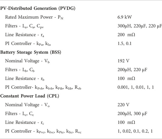
TABLE 2. Parameters of PV-battery-load-based DC microgrid system.
To begin with, the inputs and outputs of the ANNs are gathered to be trained by measured variables, including ambient temperature (T), solar irradiance (G), the output current and voltage of PV arrays (ipv and vpv), the output current of battery (ib), the running current of CPL (ic), the DC bus voltage (vdc), and the manually labelled corresponding operation modes (Mi, i =1,2, … ,6). To simulate the random and intermittent disturbances of the DC microgrid, the variations of the inputs and outputs of the system, including ambient temperature, solar irradiance (Sidi et al., 2015) and various consumed power loads, are set to generate 600 groups of environmental states. For each state, ten groups are collected and marked to ensure the accuracy of the data collection. As the nonlinear dynamic stability analysis method in this paper is a steady-state analysis, a simulation duration of 5 s is chosen, ten sets of data are initially sampled at intervals of 0.2 s between 3 and 5 s, and one set of the sampled datasets is selected as the final original datasets to guarantee that all the data sets are in the stable or unstable states. Moreover, stratified sampling (Qian et al., 2009) is employed to keep the distribution of data consistent as much as possible to ensure that each category within a dataset is adequately represented in the sample, and the datasets are divided into 85% training sets and 15% test sets.
Because we are dealing with relatively small datasets with six classes, the choice of hyper-parameters is harder and more important. For training the networks, the stochastic gradient descent (SGD) optimizer is utilized, and we set weight decay of 2 × 10⁻⁵ of SGD, which is equivalent to L2 regularization, to improve the model’s generalization capacity (Loshchilov and Hutter, 2017). There are several hyper-parameters that need to be fine-tuned, i.e., number of hidden layers, number of neurons, and learning rate. So, three-fold cross-validation is used to set them. We consider the number of hidden layers (l), the number of neurons (u), the learning rate (η), with momentum of 0.8, 2000 epochs, and other default parameters throughout.
We introduce the multi-label Accuracy measure, as defined in (Read et al., 2011), (Read and Perez-Cruz, 2014), to report the performance of ANNs with different hyper-parameters as follows:
where yi is the true set of labels, and
The results in Figure 5 show the Loss and Accuracy to evaluate the performance of a varying number of hidden layers l
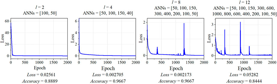
FIGURE 5. Loss of training process, and Accuracy of test datasets, for the number of hidden layers l
There are other hyper-parameters available to be tuned: the number of neurons in hidden layers (u = [u1, u2, u3, u4]) and learning rate (η), where u1∼ u4 denote the number of neurons in the corresponding layer. The results of (Loss, Accuracy) for varying number of hidden neurons and learning rate η
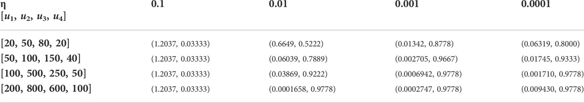
TABLE 3. (Loss, Accuracy) for varying number of hidden neurons (u = [u1, u2, u3, u4]) and learning rate (η).
The trained ANNs are then used to assist in calculating the nonlinear stability margin to monitor the DC bus voltage when both input and output conditions of the system change simultaneously. This paper simulates a real DC microgrid system by integrating fluctuations in solar radiation and ambient temperature of the photovoltaic panel and variations in the power consumption of the CPLs. Figures 6A,B depicts the variation of input and output conditions, and the variation of solar irradiance and ambient temperature in Figure 6A corresponds to the reference (Sidi et al., 2015). To study the effect of the irradiance and temperature variations throughout the day on the operation of the DC microgrid system, we compressed the data in the time range of a day into 6 s to facilitate simulation.
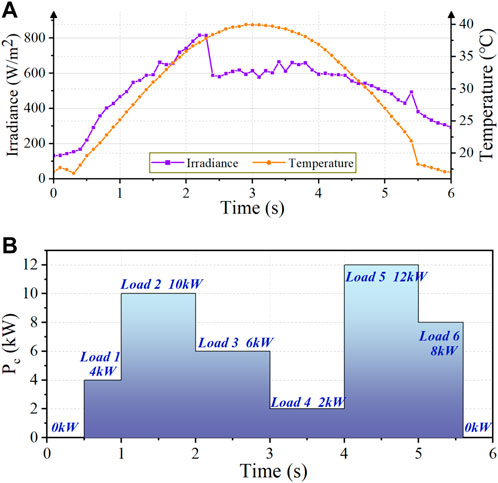
FIGURE 6. Variation of input and output conditions of the studied DC microgrid system. (A) Variation of solar irradiance and ambient temperature. (B) Variation of CPLs.
The dynamic of the calculated stability margin ε under varying input and output conditions is depicted in Figure 7. This figure shows that overall when the solar radiation and ambient temperature gradually vary, the calculated stability margin ε varies slightly. In contrast, a quick shift in CPL will have a major impact on the stability margin ε. In practice, the linked load’s power consumption frequently fluctuates abruptly, indicating that the change in CPL’s power consumption significantly impacts on system stability. At 0–0.5s and 5.5∼6s, the CPL is 0kW, which implies that the system output is zero, and the stability margin is about 0.87, which is relatively the largest, indicating that the system is most stable at this time. When the loads of 4kW and 10 kW are connected respectively at 0.5s and 1s, the stability margins decrease to around 0.59 and 0.032, respectively. In the period of 1–2 s, the stability margin falls to about 0.032, and the DC bus voltage waveform fluctuates by 2.5% in amplitude. In addition, we calculate that under the same climatic conditions for 1–2 s when the constant power load was 9.6kW, the DC bus voltage fluctuated by about 2.5%, and the stability margin was 0.091. To ensure that the bus voltage fluctuates by less than 2.5%, we have set the critical value stability margin at 0.1. The access load is then reduced to 6kW, and the stability margin increases at 2 s. Additionally, when solar radiation drops sharply, the stability margin will increase sharply, such as at 2.3 s, as the stability margin jumps from 0.37 to 0.52. After that, the access load grows abruptly to 12 kW at 4 s, leading the stability margin to decrease to approximately -0.13 and the system to lose stability. Finally, the system resumes steady operation at 5s and 5.5s when the load is gradually lowered to 6 kW and 0kW, and ε is correspondingly increased to around 0.32 and 0.87. From the preceding analysis, it can be concluded that the DC microgrid’s stability declines with rising CPL, and there is a critical CPL value.

FIGURE 7. The dynamic variation of stability margin during conditions changing.
The corresponding time domain simulation is conducted to further verify the correctness of the proposed voltage stability monitoring method, and Figures 8A,B depicts the dynamic waveforms of the DC bus voltage and the BSS charging and discharging current. In this figure, the time-domain waveforms of the DC bus voltage and BSS current vary in response to the weather conditions input to the system and the power consumed by the CPL, which appears to be operating steadily throughout the process. However, these dynamic waveforms appear to not match the stability margin calculation. Therefore, the typical states I ∼ VI, in which the system is in different degrees of stability, are selected and marked in Figure 7 and Figure 8. Figure 9 shows the zoomed waveforms corresponding to the DC bus voltage during the appropriate state.
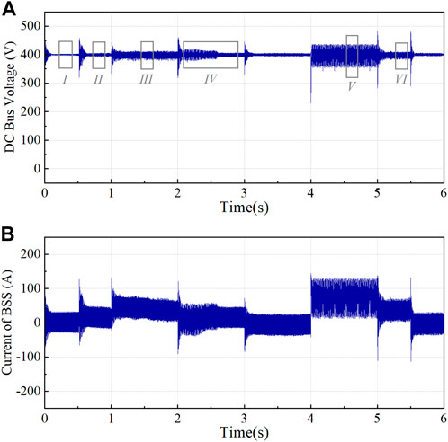
FIGURE 8. System Dynamics during conditions changing. (A) Dynamic of DC bus voltage. (B) Dynamic of BSS current.
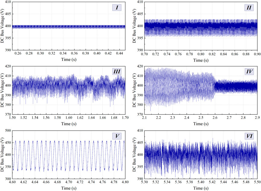
FIGURE 9. Zoomed dynamic of DC bus voltage during conditions changing.
In Figure 9, the amplified waveforms of states I and II are both stable, and the DC bus voltage fluctuation amplitude in state II is larger than that in state I, which corresponds to the variation of the stability margin in Figure 7. In state III, the fluctuation range of the DC bus voltage is greater, and it contains some harmonics. The stability margin is below critical stability margin of εr = 0.1 and close to 0, indicating that the system is in a critical stability state. In addition, it shows that the critical stability margin is set at a reasonable value, and an early warning should be given to alert of potential instability. The DC bus voltage continues to fluctuate in state IV under the disturbance of CPL. However, the waveform fluctuates less due to the sudden drop in solar irradiance, which is consistent with the calculation result of the stability margin. As a result of the sudden increase in CPL, the DC bus voltage of state V exhibits constant-amplitude oscillations, at which time the stability margin is less than 0, and the system is unstable. Lastly, when the CPL is reduced, the DC bus voltage waveform of state VI ceases to oscillate. However, this may be due to the previous oscillation as the bus voltage has some glitches at this time, but it is overall stable. In conclusion, the time domain waveform results demonstrate the precision of the proposed voltage stability monitoring method.
5 Conclusion
This paper proposes a voltage monitoring method using ANN-aided nonlinear dynamic stability analysis for the DC microgrid. In the proposed method framework, the trained neural network generates the predicted operating mode of the DC microgrid, which is then input into the nonlinear analysis algorithm based on the Poincaré map theory to calculate the stability margin. Moreover, this method makes the theoretical analysis of Poincaré mapping flexible and convenient, thereby solving the problem that the iterative mapping order is difficult to determine as the number of power electrons rises. A thorough introduction to neural network hyper-parameters tuning is provided. The theoretical and simulation analyses further verify the accuracy of the proposed analysis method. In the case study, it is found that when the solar irradiance and ambient temperature of the PVDG or the CPL change greatly, the stability margin varies from close to 1 to a negative value, which indicates that changes in the behaviour of the input and output interfaces could cause the DC microgrid to be unstable, such as oscillations in the bus voltage. Also, this nonlinear intelligent approach can be extended to other relatively small-scale power electronics-dominated power systems to monitor their stability. As for the larger system, the approximate modeling or more complex neural networks may be considered to utilized in the future study.
Data availability statement
The original contributions presented in the study are included in the article/supplementary material, further inquiries can be directed to the corresponding author.
Author contributions
SS: inspiration and implement of algorithm, simulation validation, manuscript writing and reviewing; CT: simulation validation, and manuscript reviewing; GH: supervision, and manuscript reviewing; DX: inspiration of algorithm, supervision, and manuscript reviewing.
Funding
This work was supported in part by National Natural Science Foundation of China under Grant 52077137, 51677114.
Conflict of interest
The authors declare that the research was conducted in the absence of any commercial or financial relationships that could be construed as a potential conflict of interest.
Publisher’s note
All claims expressed in this article are solely those of the authors and do not necessarily represent those of their affiliated organizations, or those of the publisher, the editors and the reviewers. Any product that may be evaluated in this article, or claim that may be made by its manufacturer, is not guaranteed or endorsed by the publisher.
References
Ahmadi, H., and Kazemi, A. (2020). The Lyapunov-based stability analysis of reduced order micro-grid via uncertain LMI condition. Int. J. Electr. Power & Energy Syst. 117, 105585. doi:10.1016/j.ijepes.2019.105585
Ahmed, M., Meegahapola, L., Vahidnia, A., and Datta, M. (2020). Stability and control aspects of microgrid architectures–A comprehensive review. IEEE Access 8, 144730–144766. doi:10.1109/access.2020.3014977
Aroudi, A. E., Debbat, M., and Martinez-Salamero, L. (2007). Poincaré maps modeling and local orbital stability analysis of discontinuous piecewise affine periodically driven systems. Nonlinear Dyn. 50, 431–445. doi:10.1007/s11071-006-9190-1
Eberlein, S., and Rudion, K. (2021). Small-signal stability modelling, sensitivity analysis and optimization of droop controlled inverters in LV microgrids. Int. J. Electr. Power & Energy Syst. 125, 106404. doi:10.1016/j.ijepes.2020.106404
Geng, S., and Hiskens, I. A. (2019). Second-order trajectory sensitivity analysis of hybrid systems. IEEE Trans. Circuits Syst. I. 66 (5), 1922–1934. doi:10.1109/tcsi.2019.2903196
Gomez, F., Rajapakse, A., Annakkage, U., and Fernando, I. (2011). “Support vector machine-based algorithm for post-fault transient stability status prediction using synchronized measurements,” in 2011 IEEE Power and Energy Society General Meeting, Detroit, MI, USA, July 24-28.
Holari, Y. T., Taher, S. A., and Mehrasa, M. (2021). Power management using robust control strategy in hybrid microgrid for both grid-connected and islanding modes. J. Energy Storage 39, 102600. doi:10.1016/j.est.2021.102600
Khodamoradi, A., Liu, G., Mattavelli, P., Caldognetto, T., and Magnone, P. (2019). Analysis of an online stability monitoring approach for DC microgrid power converters. IEEE Trans. Power Electron. 34 (5), 4794–4806. doi:10.1109/tpel.2018.2858572
Liu, W., Wen, Y., Yu, Z., and Yang, M. (2016). Large-margin softmax loss for convolutional neural networks. arXiv preprint arXiv:1612.02295.
Loshchilov, I., and Hutter, F. (2017). Decoupled weight decay regularization. arXiv preprint arXiv:1711.05101.
Lu, X., Sun, K., Guerrero, J. M., Vasquez, J. C., Huang, L., and Wang, J. (2015). Stability enhancement based on virtual impedance for DC microgrids with constant power loads. IEEE Trans. Smart Grid 6 (6), 2770–2783. doi:10.1109/tsg.2015.2455017
Marx, D., Magne, P., Nahid-Mobarakeh, B., Pierfederici, S., and Davat, B. (2012). Large signal stability analysis tools in DC power systems with constant power loads and variable power loads—a review. IEEE Trans. Power Electron. 27 (4), 1773–1787. doi:10.1109/tpel.2011.2170202
Maxwell, A., Li, R., Yang, B., Weng, H., Ou, A., Hong, H., et al. (2017). Deep learning architectures for multi-label classification of intelligent health risk prediction. BMC Bioinforma. 18 (14), 523–131. doi:10.1186/s12859-017-1898-z
Mehran, K., Giaouris, D., and Zahawi, B. (2009). Modeling and stability analysis of closed loop current-mode controlled cuk converter using takagi-sugeno fuzzy approach. IFAC Proc. Vol. 42 (7), 223–228. doi:10.3182/20090622-3-uk-3004.00043
Moreno-Font, V., El Aroudi, A., Calvente, J., Giral, R., and Benadero, L. (2009). Dynamics and stability issues of a single-inductor dual-switching DC–DC converter. IEEE Trans. Circuits Syst. I. 57 (2), 415–426. doi:10.1109/tcsi.2009.2023769
Qian, L., Zhou, G., Kong, F., and Zhu, Q. (2009). “Semi-supervised learning for semantic relation classification using stratified sampling strategy,” in Proceedings of the 2009 conference on empirical methods in natural language processing, Singapore, Aug 6-7, 1437–1445.
Rahimi, A. M., and Emadi, A. (2009). An analytical investigation of DC/DC power electronic converters with constant power loads in vehicular power systems. IEEE Trans. Veh. Technol. 58 (6), 2689–2702. doi:10.1109/tvt.2008.2010516
Read, J., and Perez-Cruz, F. (2014). Deep learning for multi-label classification. arXiv preprint arXiv:1502.05988.
Read, J., Pfahringer, B., Holmes, G., and Frank, E. (2011). Classifier chains for multi-label classification. Mach. Learn. 85 (3), 333–359. doi:10.1007/s10994-011-5256-5
Seth, S., and Banerjee, S. (2020). Electronic circuit equivalent of a mechanical impacting system. Nonlinear Dyn. 99, 3113–3121. doi:10.1007/s11071-019-05457-w
Sidi, C. El B. E., Ndiaye, M. L., Ndiaye, A., and Ndiaye, P. A. (2015). Outdoor performance analysis of a monocrystalline photovoltaic module: Irradiance and temperature effect on exergetic efficiency. Int. J. Phys. Sci. 10 (11), 351–358. doi:10.5897/ijps2015.4356
Tan, B., Yang, J., Tang, Y., Jiang, S., Xie, P., and Yuan, W. (2019). A deep imbalanced learning framework for transient stability assessment of power system. IEEE Access 7, 81759–81769. doi:10.1109/access.2019.2923799
Tian, Z., Shao, Y., Sun, M., Zhang, Q., Ye, P., and Zhang, H. (2022). Dynamic stability analysis of power grid in high proportion new energy access scenario based on deep learning. Energy Rep. 8 (6), 172–182. doi:10.1016/j.egyr.2022.03.055
Toro, V., Mojica-Nava, E., and Rakoto-Ravalontsalama, N. (2021). Stability analysis of DC microgrids with switched events. IFAC-PapersOnLine 54 (14), 221–226. doi:10.1016/j.ifacol.2021.10.356
Tse, C. K., and Di Bernardo, M. (2002). Complex behavior in switching power converters. Proc. IEEE 90 (5), 768–781. doi:10.1109/jproc.2002.1015006
Vanfretti, L., and Narasimham Arava, V. S. (2020). Decision tree-based classification of multiple operating conditions for power system voltage stability assessment. Int. J. Electr. Power & Energy Syst. 123, 106251. doi:10.1016/j.ijepes.2020.106251
Wang, B., Sun, K., and Kang, W. (2018). Nonlinear modal decoupling of multi-oscillator systems with applications to power systems. IEEE Access 6, 9201–9217. doi:10.1109/access.2017.2787053
Wang, Y., Xu, L., Chen, L., and Zhou, J. (2020). Discrete iterative map model-based stability analysis of capacitor current ripple-controlled SIDO CCM buck converter. IEEE J. Emerg. Sel. Top. Power Electron. 8 (4), 3272–3280. doi:10.1109/jestpe.2020.2972651
Wu, H., Pickert, V., Ma, M., Ji, B., and Zhang, C. (2020). Stability study and nonlinear analysis of DC–DC power converters with constant power loads at the fast timescale. IEEE J. Emerg. Sel. Top. Power Electron. 8 (4), 3225–3236. doi:10.1109/jestpe.2020.2966375
Xia, Y., Wei, W., Yu, M., and Wang, P. (2019). Stability analysis of PV generators with consideration of P&O-based power control. IEEE Trans. Ind. Electron. 66 (8), 6483–6492. doi:10.1109/tie.2018.2864695
Xia, Y., Wei, W., Long, T., Blaabjerg, F., and Wang, P. (2020). New analysis framework for transient stability evaluation of DC microgrids. IEEE Trans. Smart Grid 11 (4), 2794–2804. doi:10.1109/tsg.2020.2964583
Xie, W., Han, M., Cao, W., Guerrero, J. M., and Vasquez, J. C. (2021). System-level large-signal stability analysis of droop-controlled DC microgrids. IEEE Trans. Power Electron. 36 (4), 4224–4236. doi:10.1109/tpel.2020.3019311
Zhang, Z., Yang, X., Zhao, S., Wu, D., Cao, J., Gao, M., et al. (2022). Large-signal stability analysis of islanded DC microgrids with multiple types of loads. Int. J. Electr. Power & Energy Syst. 143, 108450. doi:10.1016/j.ijepes.2022.108450
Zia, M. F., Elbouchikhi, E., and Benbouzid, M. (2019). Optimal operational planning of scalable DC microgrid with demand response, islanding, and battery degradation cost considerations. Appl. Energy 237, 695–707. doi:10.1016/j.apenergy.2019.01.040
Keywords: voltage monitoring, nonlinear stability analysis, artificial neural network, poincaré map, DC microgrid
Citation: Sun S, Tang C, Hailati G and Xie D (2023) Voltage monitoring based on ANN-aided nonlinear stability analysis for DC microgrids. Front. Energy Res. 10:1045809. doi: 10.3389/fenrg.2022.1045809
Received: 16 September 2022; Accepted: 21 October 2022;
Published: 10 January 2023.
Edited by:
Weiye Zheng, South China University of Technology, ChinaReviewed by:
Xinran Zhang, Central Conservatory of Music, ChinaZhiyuan Tang, Sichuan University, China
Xue Lyu, University of Wisconsin-Madison, United States
Copyright © 2023 Sun, Tang, Hailati and Xie. This is an open-access article distributed under the terms of the Creative Commons Attribution License (CC BY). The use, distribution or reproduction in other forums is permitted, provided the original author(s) and the copyright owner(s) are credited and that the original publication in this journal is cited, in accordance with accepted academic practice. No use, distribution or reproduction is permitted which does not comply with these terms.
*Correspondence: Da Xie, eGllZGFAc2p0dS5lZHUuY24=