 Andrei Kulikovsky
- Forschungszentrum Jülich GmbH, Theory and Computation of Energy Materials (IEK–13), Institute of Energy and Climate Research, Jülich, Germany
Impedance of all oxygen transport processes in PEM fuel cell has negative real part in some frequency domain. A kernel for calculation of distribution of relaxation times (DRT) of a PEM fuel cell is suggested. The kernel is designed for capturing impedance with negative real part and it stems from the equation for impedance of oxygen transport through the gas-diffusion transport layer (doi:10.1149/2.0911509jes). Using recent analytical solution for the cell impedance, it is shown that DRT calculated with the novel K2 kernel correctly captures the GDL transport peak, whereas the classic DRT based on the RC-circuit (Debye) kernel misses this peak. Using K2 kernel, analysis of DRT spectra of a real PEMFC is performed. The leftmost on the frequency scale DRT peak represents oxygen transport in the channel, and the rightmost peak is due to proton transport in the cathode catalyst layer. The second, third, and fourth peaks exhibit oxygen transport in the GDL, faradaic reactions on the cathode side, and oxygen transport in the catalyst layer, respectively.
1 Introduction
Electrochemical impedance spectroscopy provides unique opportunity for testing and characterization of PEM fuel cells without interruption of current production mode (Lasia, 2014). A classic approach to interpretation of EIS data is construction of equivalent electric circuit having impedance spectrum close to the measured one. However, a more attractive option provides the distribution of relaxation times (DRT) technique. Note that DRT is sometimes called distribution function of relaxation times.
In the context of PEM fuel cell studies, the idea of DRT can be explained as follows. To a first approximation, PEM fuel cell impedance Z can be modeled as impedance of a parallel RC circuit
where ω is the angular frequency of applied AC signal. This approximation corresponds to the cell with ideal (fast) transport of reactants in all transport media (Kulikovsky, 2017). In that case, R describes Tafel resistivity of the oxygen reduction reaction (ORR), and C represents the superficial double-layer capacitance of the electrode.
In general, to calculate transport contributions to cell impedance, one has to develop a transport model for the ORR reactants. However, if information on transport resistivities and characteristic frequencies suffices, DRT provides a simpler option. Denoting RC = τ, multiplying the right side of Eq. 1 by nonnegative function γ(τ) and integrating over τ, we get
where Rpol is the total polarization resistivity of the cell, and the function γ is the DRT of impedance Z. Mathematically, Eq. 2 means expansion of Z(ω) into infinite sum of RC impedances, with the resistivity of each elementary RC circuit being Rpolγ dτ. The function
under integral in Eq. 2 is usually called “Debye model” (Barsoukov and Macdonald, 2018). Eq. 2 can also be considered as integral transform of γ(τ), which justifies the term “RC kernel” for Eq. 3.
Quite evidently, DRT of a single parallel RC circuit is Dirac delta function γ = δ(τ − τ*) positioned at τ* = RC. This example illustrates the main feature of DRT: it converts any RC-like impedance into a single, more or less smeared on the τ scale δ-like peak.
All transport processes in a fuel cell eventually are linked to the double-layer capacitance in the catalyst layer; thus, it is usually assumed that impedance of every process is not far from impedance of a parallel RC circuit. That means that the DRT of a PEMFC is expected to consist of several delta-like peaks. As the regular frequency f = 1/(2πτ), it is convenient to plot γ(f) instead of γ(τ). Position of each γ(f) peak marks a characteristic frequency of the respective transport process and
gives the contribution of process resistivity to the total cell polarization resistivity Rpol. Here, τn and τn+1 are the peak boundaries on the τ scale.
Fuel cell impedance is usually measured on equidistant in log-scale frequency mesh {fn, n = 1, … , N}, with ln (fn+1) − ln (fn) being independent of n. From numerical perspective, it is beneficial to deal with the function G(τ) satisfying to
where the term R∞ is added to describe pure ohmic (high-frequency) fuel cell resistivity. Clearly, γ = G/τ, and Eq. 4 in terms of G takes the form
where the frequencies fn = 1/(2πτn+1) and fn+1 = 1/(2πτn) mark the peak boundaries. Note that Eqs 4, 6 return a single peak resistivity if the DRT peaks are not overlapped; otherwise, Rn would represent the sum of overlapped peak resistivities. The problem of overlapped peak resistivity is alleviated if the DRT in analytical form is found, as in, for example, the ISGP method (Avioz Cohen et al., 2021).
Setting in Eq. 5 ω = 0 and taking into account that Z (0) − R∞ = Rpol, we see that G obeys to normalization condition
In the following, Eq. 5 will be discussed, as G is usually used instead of γ in practical calculations.
DRT technique, Eq. 2, was invented by Fuoss and Kirkwood (1941) in the context of polymer materials impedance and brought to the fuel cell community seemingly by Schichlein et al. (2002). Since 2002, a lot of works from the group of Ivers–Tiffée have been devoted to deciphering of solid oxide fuel cell spectra by means of DRT [see a review (Ivers-Tiffee and Weber, 2017)]. Analysis of PEMFC impedance spectra using DRT is a relatively new field (Heinzmann et al., 2018; Avioz Cohen et al., 2021; Reshetenko and Kulikovsky, 2021; Wang et al., 2021). Heinzmann et al. (2018) measured impedance spectra of a small (1 cm2) laboratory PEMFC and studied DRT peak behavior depending on cell temperature, relative humidity (RH), oxygen concentration, and current density. They obtained DRT with up to five peaks; the leftmost on the frequency scale peak P1 was attributed to oxygen diffusion in the gas-diffusion and cathode catalyst layers (CCLs). Avioz Cohen et al. (2021) performed impedance measurements of a 5-cm2 cell varying temperature, RH, and current density. The calculated DRT consisted of four peaks, attributed (in ascending frequencies) to (1) oxygen transport in the GDL/CCL, (2) ORR, (3) proton transport in the CCL, and (4) proton transport in membrane. Note that Heinzmann et al. and Cohen et al. used different codes for DRT calculation. Wang et al. (2021) measured impedance spectra of application-relevant 25-cm2 PEMFC and obtained a three–peak DRT; the lowest frequency peak was attributed to oxygen diffusion processes in the cell. In our recent work (Reshetenko and Kulikovsky, 2021), DRT spectra of a low-Pt PEMFC have been reported; we attributed the low-frequency peak to oxygen transport in the GDL and, possibly, in the channel.
In PEMFCs, the supplied oxygen (air) is transported through the four quite different media: channel, GDL, open pores of the CCL, and finally through Nafion film covering Pt/C agglomerates. One therefore could expect four corresponding peaks in the DRT spectra. However, in Heinzmann et al. (2018), Avioz Cohen et al. (2021), and Wang et al. (2021), a single oxygen transport peak has been reported. There are two options to explain this result: either some of the oxygen transport peaks overlap with each other (or with the ORR peak) and DRT is not able to separate them, or the codes used were unable to resolve all the transport processes. It is important to note that the code for DRT calculation of Wan et al. (2015) used in Heinzmann et al. (2018) and Wang et al. (2021), the ISGP code (Hershkovitz et al., 2011) used in Avioz Cohen et al. (2021), and our code using Tikhonov regularization (Tikhonov, 1995) in combination with NNLS solver (Kulikovsky, 2020a; Kulikovsky, 2021a) are based on the RC kernel, Eq. 5.
The real part of RC-circuit impedance, Eq. 1, is positive, and the imaginary part is negative. This imposes limits on functions Z, which could be represented by Eq. 5. For example, impedance of an inductive loop cannot be expanded in infinite series of RC impedances, as the imaginary part of inductive impedance is positive. Quite similarly, the impedance Z having negative real part in some frequency domain also cannot be represented by Eq. 5.
Below, we show that the DRT calculated with RC kernel could completely miss some of the transport peaks in PEMFC spectra. An alternative K2 kernel better capturing oxygen transport processes in the cell cathode is suggested. The kernel is illustrated by calculation of DRT of the recent analytical PEM fuel cell impedance spectrum (Kulikovsky, 2021b). Finally, we show that the new kernel well separates the channel, GDL, and ORR peaks in the DRT spectra of a standard Pt/C-based PEM fuel cell.
2 Model: K2 Kernel
Below, the following dimensionless variables will be used
Here, t* is the characteristic time of double-layer charging
c is the oxygen concentration,
Analytical GDL impedance
where μ is the constant parameter
Eq. 10 has been obtained from the general expression for the cathode side impedance in the limit of infinite air flow stoichiometry (Kulikovsky and Shamardina, 2015). Eq. 10 is a Warburg finite-length impedance divided by the factor
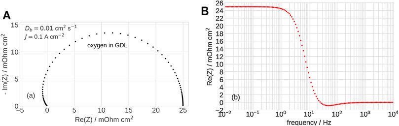
FIGURE 1. (A) Nyquist spectrum of the gas-diffusion layer impedance, Eq. 10. (B) Frequency dependence of the real part of impedance in (A). Parameters for calculations are listed in Table 1.
Impedance of oxygen transport in channel, Appendix Eq. A1, and in the CCL (Kulikovsky, 2017) also exhibits negative real part (Figure 2). Last but not least, in low-Pt cells, an important role plays oxygen transport through a thin Nafion film covering Pt/C agglomerates in the CCL (Greszler et al., 2012; Weber and Kusoglu, 2014; Kongkanand and Mathias, 2016). The spectrum of this transport layer is quite similar in shape to the spectrum in Figure 1 (Kulikovsky, 2021a). Thus, all the oxygen transport processes in a PEMFC cannot be described by the standard RC kernel, and another kernel suitable for description of impedance elements with the negative real part is needed.
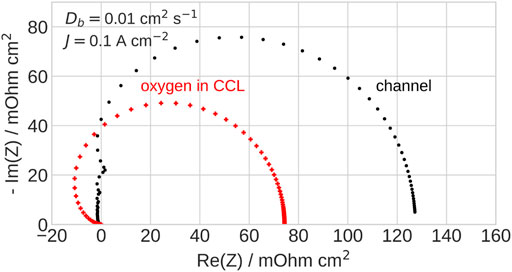
FIGURE 2. Nyquist spectra of the channel impedance, Appendix Eq. A1 and of impedance of oxygen transport in the CCL (Kulikovsky, 2017).
In a standard PEMFC, unless the cell current density is small, the DRT peaks of oxygen transport in the GDL, CCL, and channel are expected to locate at frequencies below the frequency fct of faradaic (charge transfer) processes. Thus, to capture the oxygen transport peaks, correction for the negative real part of impedance is needed in the range of frequencies f < fct. The kernel K2 suggested in his work consists, thus, of two parts:
where f* ≃ fct is the threshold frequency. Selection of optimal f* is discussed below. A function similar to impedance of a transport layer (TL) (10) forms the low-frequency part of K2; the real part of this function is negative at ωτ > 1.81052. The high-frequency (RC) part of K2 is the standard RC-circuit kernel. Switching between TL and RC kernels is necessary, as the TL part itself does not describe well RC-circuit impedance (see below). The real part of GDL impedance becomes negative at ≃20 Hz (Figure 1B), while the imaginary part at this frequency is quite large (Figure 1A). This shape of impedance around and below 20 Hz is thus far from the RC-circuit impedance and the TL kernel is needed to “recognize” this shape. At higher frequencies, transport impedances tend to zero, and the Debye kernel works better. The idea behind Eq. 12 is thus to expand the low-frequency components of cell impedance using the TL kernel and the high-frequency components using the standard RC kernel.
It is convenient to combine Eq. 12 into one function
where α is a step function of the frequency f
H(x) is the Heaviside step function, and ϵ = 10–10 is a small parameter to avoid zero division error. Parameter α therefore changes from 1 to 0 at the threshold frequency f = f*. With α → 0, the Warburg factor in Eq. 13 tends to unity:
and hence the α function serves as a switch between the two kernels in Eq. 12.
Setting in Eq. 16 ω → 0, it is easy to show that G still obeys to normalization conditions, Eq. 7.
3 Numerical Results and Discussion
3.1 Synthetic Impedance Tests
Figure 3 shows the imaginary part of the RC-circuit impedance for R = 1, C = 0.01 and the DRT calculated using Eq. 16, and α = 1 for all frequencies (TL kernel). As can be seen, the main peak is positioned correctly at the frequency 1/(2πRC); however, the DRT spectrum exhibits three phantom peaks located to the right of the main peak. It is worth noting that quite similarly, the RC kernel generates several phantom peaks in the DRT of Warburg finite-length impedance (Kulikovsky, 2020a), that is, no single kernel is able to correctly represent DRT of all impedance components.
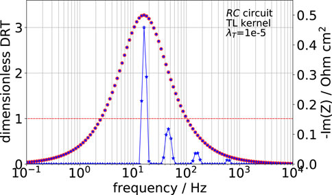
FIGURE 3. DRT (solid line, blue stars, left axis) and imaginary part of RC-circuit impedance 1/(1 + 10−2iω) (blue dots, right axis) calculated with Eq. 16 and α = 1 for all frequencies. Open red circles show imaginary part reconstructed from the calculated DRT using Eq. 16. Dashed red line plots α = 1 for this calculation.
In a standard PEMFC, the characteristic frequencies of channel and GDL impedance are approximately 1 and 10 Hz, respectively (Kulikovsky, 2021b). Thus, the typical value of the threshold frequency f* in Eq. 14 should be about 10 Hz; however, the exact value can always be selected simply looking at the calculated DRT spectrum. In standard PEMFCs operated at oxygen stoichiometry of 2, the faradaic DRT peak is located to the right of the GDL transport peak on the log-frequency scale (see below).
Analytical impedance

FIGURE 4. (A) DRT calculated with the RC kernel (solid line, left axis) using imaginary part of the total cathode side impedance, Appendix Eq. A6 (blue dots, right axis). Red open circles—
The spectrum of
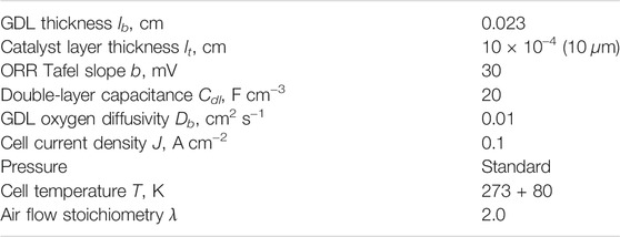
TABLE 1. The base–case cell parameters used in calculations.
Figure 4A shows the DRT spectrum of
Figure 4B displays the DRT calculated with the “pure” TL kernel, Eq. 12. The GDL peak is resolved, and the quality of reconstructed imaginary part is much better; however, phantom high-frequency peaks to the right of the faradaic peak are clearly seen (cf. Figure 3). Figure 4C shows the DRT spectrum calculated using the K2 kernel with the threshold frequency of 10 Hz; the GDL peak is well resolved, and the phantom peaks vanish. It is worth mentioning that the real part of the total cell impedance is always positive due to positive contributions of the faradaic and proton transport impedances. However, the Debye kernel fails to recognize the transport impedances having negative real part, as the whole shape of this impedance strongly deviates from the RC circuit one. The result in Figure 4C shows that in order to be recognized, the DRT peak corresponding to the process with negative real part must be fully “covered” by the TL kernel. The respective DRT peak frequency corresponds to the peak value of the imaginary part of impedance (cf. Figures 4C,D).
Table 2 shows the resistivities, Eq. 6, corresponding to individual peaks in Figure 4. As can be seen, K2 kernel provides good estimate of the channel and faradaic resistivities; however, the GDL resistivity Rgdl is underestimated by 30%. Nonetheless, as the contribution of Rgdl is small, the 30% accuracy could be tolerated.
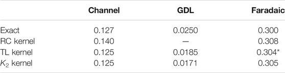
TABLE 2. Channel, GDL, and faradaic resistivities (Ω cm2) resulting from DRT, Eq. 6. Star ∗ indicates the value calculated as a sum of faradaic and all high-frequency peaks in Figure 4B. The first row shows exact data calculated with Appendix Eqs. A13.
3.2 Real PEMFC Spectra
A crucial check for the new kernel is calculation of DRT of a real PEM fuel cell. Impedance spectra of a standard Pt/C-based PEMFC have been measured in the frequency range of 0.1 to approximately 103 Hz with 11 points per decade. The cell geometrical parameters and operating conditions are listed in Table 3; note that the air flow stoichiometry was 2 in this set of measurements. The impedance points in the frequency range above ≃ 103 Hz have been discarded due to effect of cable inductance. More details on experimental setup and measuring procedures can be found in Reshetenko and Kulikovsky (2019).
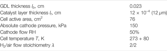
TABLE 3. PEM fuel cell geometric and operating parameters.
Figure 5 shows DRT spectra calculated with the real part of measured impedance using the RC kernel. Figure 6 shows the respective peak frequencies and resistivities. The DRT spectra in Figures 5A–C exhibit four peaks, whereas in Figure 5D, the most high-frequency peak disappears. This peak represents proton transport in the CCL, and at high cell currents, it shifts to frequencies that have been discarded. The characteristic frequency f4 of proton transport in the CCL is given by Kulikovsky (2020b)

FIGURE 5. DRT (solid line, left axis) calculated with the RC kernel using real part of the experimental PEMFC impedance (blue dots, right axis) for the current densities (A) 100, (B) 200, (C) 400, and (D) 800 mA cm−2. Red open circles—

FIGURE 6. Frequency (blue curves, left axis) and resistivity (red curves, right axis) of the DRT peaks calculated using RC kernel (Figure 5) versus mean cell current density J. (A) first peak, (B) second peak and (C) third and fourth peaks.
With the typical values of σp ≃ 0.01 S cm−1 and Cdl ≃ 20 F cm−3 [Ref. (Reshetenko and Kulikovsky, 2019)], we get fp ≃ 700 Hz, which by the order of magnitude agrees with the proton peak position in Figures 5A–C. The growth of f4 with the cell current and the respective decay of the peak resistivity R4 (Figure 6C) is due to growing amount of liquid water improving the CCL proton conductivity.
The leftmost peak in Figures 5A–D represents impedance due to oxygen transport in the cathode channel. The characteristic frequency f1 of this peak linearly increases with the cell current density (Figure 6A), which is a signature of channel impedance (Kulikovsky, 2021b).
The highest, second peak in the DRT spectra (Figures 5A–D) represents the contributions of ORR and oxygen transport in the GDL (see below). In the absence of strong oxygen and proton transport limitations, the ORR resistivity is given by
which follows the Tafel law. Qualitatively, the shape of second peak resistivity R2 follows the trend of Eq. 18 due to dominating contribution of ORR resistivity to this peak (Figure 6B). Note that the separate GDL peak is not resolved by the RC kernel.
The third CCL peak in Figures 5A–D is most probably due to oxygen transport in the CCL pores. For the estimate. we take the Warburg finite-length formula for the transport layer frequency fW
where D is the oxygen diffusivity in the transport layer of the thickness l. Setting fW = 35 Hz (Figure 5A) and l = lt, for the oxygen diffusion coefficient in the CCL, we get Dox ≃ 1.2 ⋅ 10–4 cm2 s−1, which agrees with measurements (Reshetenko and Kulikovsky, 2019). With the growth of cell current, the peak frequency f3 rapidly shifts to 200 Hz (Figure 6C), corresponding to Dox ≃ 7 ⋅ 10–4 cm2 s−1. This result correlates with the growth of Dox resulting from fitting of physics-based impedance model to the PEMFC cell spectra (Reshetenko and Kulikovsky, 2016). The mechanism of this growth yet is unclear.
Figure 7 shows the DRT of the same impedance spectra calculated with the K2 kernel. The properties of K2 kernel are immediately seen: setting of the threshold frequency f* in Eq. 14 just to the left of the “ORR + GDL” peak in Figures 5A–D splits this peak into two well-resolved peaks (Figures 7A–D). The left peak of this doublet corresponds to the GDL impedance and the right peak to the ORR impedance. With the K2 kernel, the proton transport peak is seen only at the smallest cell current density (Figure 7A), whereas at higher currents the peak vanishes, indicating its shift to the frequencies greater than 1 kHz (Figures 7B–D).
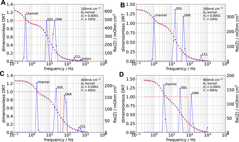
FIGURE 7. DRT (solid line, left axis) calculated with the K2 kernel using real part of the experimental PEMFC impedance (blue dots, right axis) for the current densities (A) 100, (B) 200, (C) 400, and (D) 800 mA cm−2. Red open circles—
Splitting the “CCL + GDL” peak into GDL and ORR peaks is confirmed by the behavior of peak resistivities in Figures 8B,C, respectively. The ORR peak resistivity R3 follows the trend of Eq. 18 (solid line in Figure 8C) with the ORR Tafel slope b = 30 mV, which is a typical value for Pt/C cells (Neyerlin et al., 2006). The GDL resistivity R2 decreases in the range of cell currents 100 to 400 mA cm−2 and remains nearly constant at higher currents (Figure 8B). Using again the Warburg formula Eq. 19, with l = lb = 230 ⋅ 10–4 cm and the frequency between 10 and 30 Hz (Figure 8B), for the GDL oxygen diffusivity, we get quite reasonable values of Db ≃ 0.013–0.033 cm2 s−1. The increase of Db in the range of 100 to 400 mA cm−2 is probably due to growing air flow velocity in the channel at the constant stoichiometry, which facilitates liquid droplets removal from the GDL.
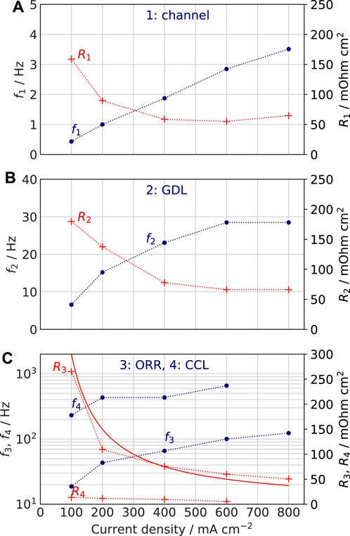
FIGURE 8. Frequency and resistivity of the DRT peaks calculated using K2 kernel (Figure 7) versus mean cell current density J. Solid line in (C) is the Tafel ORR resistivity RORR = b/J plotted with the Tafel slope b = 0.03 V (69 mV/decade). (A) first peak, (B) second peak and (C) third and fourth peaks.
Comparing the GDL peaks in Figures 7A,B one can see that the area under this peak increases with the cell current density. However, the area under the peak gives the fraction of the respective process resistivity in the total polarization resistivity of the cell Rpol. The latter value decreases with the cell current, leading to decrease in the absolute value of RGDL (Figure 8B).
K2 kernel returns twice lower resistivity and about twice higher frequency of the CCL peak (cf. f3, R3 in Figure 6C and f4, R4 in Figure 8C). This shift leads to twice higher estimate of the CCL oxygen diffusivity, which is still acceptable (see above). Overall, confirmation of the CCL peak nature requires measurements at variable oxygen concentration and RH. An important issue is accuracy of peak resistivities calculated using the K2 kernel. Impedance spectra fitting by physics-based model seems to be the only way to get an independent estimate of the resistivities for comparison.
Over the past years, large efforts have been directed toward development of universal code capable to calculate DRT based on RC kernel, not using any a priori information on the system [see a nice review of Effendy, Song and Bazant (Effendy et al., 2020)]. However, in PEMFC studies, it would be wasteful to ignore analytical results, showing that the RC kernel alone is not well suited for DRT description of the spectra.
4 Conclusion
Impedance of all oxygen transport processes in a PEM fuel cell exhibits negative real part in some frequency range. This makes it difficult to accurately calculate the respective DRT peaks using the standard RC kernel 1/(1 + iωτ). A novel kernel K2, Eq. 13, is suggested. K2 combines the low-frequency transport layer kernel having a domain with negative real part and the standard RC kernel for description of faradaic and high-frequency processes in the cell. Calculation of DRT for analytical PEMFC impedance shows that K2 kernel captures the peak due to oxygen transport in the gas-diffusion layer, whereas the RC kernel can miss this peak. Comparison of Pt/C PEMFC DRT calculated using RC and K2 kernel shows that the K2 kernel resolves the GDL oxygen transport peak, which otherwise is merged to the ORR peak when using the standard RC kernel. Overall, the K2 spectra of a standard Pt/C PEMFC operating at the air flow stoichiometry λ = 2 consist of five peaks. In the frequency ascending order, these peaks are due to (1) oxygen transport in channel, (2) oxygen transport in the GDL, (3) faradaic reactions, (4) oxygen transport in the CCL, and (5) proton transport in the CCL. If the CCL proton conductivity is high, the peak (6) shifts to the frequencies well above 1 kHz, and it may not be resolved due to inductance of measuring system.
Data Availability Statement
The original contributions presented in the study are included in the article/Supplementary Material, further inquiries can be directed to the corresponding author.
Author Contributions
The author confirms being the sole contributor of this work and has approved it for publication.
Conflict of Interest
The author declares that the research was conducted in the absence of any commercial or financial relationships that could be construed as a potential conflict of interest.
Publisher’s Note
All claims expressed in this article are solely those of the authors and do not necessarily represent those of their affiliated organizations, or those of the publisher, the editors and the reviewers. Any product that may be evaluated in this article, or claim that may be made by its manufacturer, is not guaranteed or endorsed by the publisher.
Acknowledgments
The author is grateful to Tatyana Reshetenko (University of Hawaii) for experimental spectra used in this work and useful discussions.
References
Avioz Cohen, G., Gelman, D., and Tsur, Y. (2021). Development of a Typical Distribution Function of Relaxation Times Model for Polymer Electrolyte Membrane Fuel Cells and Quantifying the Resistance to Proton Conduction within the Catalyst Layer. J. Phys. Chem. C 125, 11867–11874. doi:10.1021/acs.jpcc.1c03667
Barsoukov, E., and Macdonald, J. R. (2018). Impedance Spectroscopy: Theory, Experiment, and Applications. 3 edition. New Jersey: John Wiley & Sons.
Effendy, S., Song, J., and Bazant, M. Z. (2020). Analysis, Design, and Generalization of Electrochemical Impedance Spectroscopy (EIS) Inversion Algorithms. J. Electrochem. Soc. 167, 106508. doi:10.1149/1945-7111/ab9c82
Fuoss, R. M., and Kirkwood, J. G. (1941). Electrical Properties of Solids. VIII. Dipole Moments in Polyvinyl Chloride-Diphenyl Systems*. J. Am. Chem. Soc. 63, 385–394. doi:10.1021/ja01847a013
Greszler, T. A., Caulk, D., and Sinha, P. (2012). The Impact of Platinum Loading on Oxygen Transport Resistance. J. Electrochem. Soc. 159, F831–F840. doi:10.1149/2.061212jes
Hansen, P. C. (1992). Analysis of Discrete Ill-Posed Problems by Means of the L-Curve. SIAM Rev. 34, 561–580. doi:10.2307/213262810.1137/1034115
Heinzmann, M., Weber, A., and Ivers-Tiffée, E. (2018). Advanced Impedance Study of Polymer Electrolyte Membrane Single Cells by Means of Distribution of Relaxation Times. J. Power Sourc. 402, 24–33. doi:10.1016/j.jpowsour.2018.09.004
Hershkovitz, S., Tomer, S., Baltianski, S., and Tsur, Y. (2011). Isgp: Impedance Spectroscopy Analysis Using Evolutionary Programming Procedure. ECS Trans. 33, 67–73. doi:10.1149/1.3589186
Ivers-Tiffee, E., and Weber, A. E. (2017). Evaluation of Electrochemical Impedance Spectra by the Distribution of Relaxation Times. J. Ceram. Soc. Jpn. 125, 193–201. doi:10.2109/jcersj2.16267
Kongkanand, A., and Mathias, M. F. (2016). The Priority and Challenge of High-Power Performance of Low-Platinum Proton-Exchange Membrane Fuel Cells. J. Phys. Chem. Lett. 7, 1127–1137. doi:10.1021/acs.jpclett.6b00216
Kulikovsky, A. A. (2017). Analytical Physics-Based Impedance of the Cathode Catalyst Layer in a PEM Fuel Cell at Typical Working Currents. Electrochimica Acta 225, 559–565. doi:10.1016/j.electacta.2016.11.129
Kulikovsky, A. (2020). Analysis of Proton and Electron Transport Impedance of a PEM Fuel Cell in H2/N2 Regime. Electrochem. Sci. Adv. 1, e202000023. doi:10.1002/elsa.202000023
Kulikovsky, A. (2021). Analytical Impedance of Oxygen Transport in the Channel and Gas Diffusion Layer of a PEM Fuel Cell. J. Electrochem. Soc. doi:10.1149/1945-7111/ac3a2d
Kulikovsky, A. (2021). Impedance and Resistivity of Low-Pt Cathode in a PEM Fuel Cell. J. Electrochem. Soc. 168, 044512. doi:10.1149/1945-7111/abf508
Kulikovsky, A. (2020). PEM Fuel Cell Distribution of Relaxation Times: a Method for the Calculation and Behavior of an Oxygen Transport Peak. Phys. Chem. Chem. Phys. 22, 19131–19138. doi:10.1039/D0CP02094J
Kulikovsky, A., and Shamardina, O. (2015). A Model for PEM Fuel Cell Impedance: Oxygen Flow in the Channel Triggers Spatial and Frequency Oscillations of the Local Impedance. J. Electrochem. Soc. 162, F1068–F1077. doi:10.1149/2.0911509jes
Neyerlin, K. C., Gu, W., Jorne, J., and Gasteiger, H. A. (2006). Determination of Catalyst Unique Parameters for the Oxygen Reduction Reaction in a PEMFC. J. Electrochem. Soc. 153, A1955–A1963. doi:10.1149/2.0471803jes10.1149/1.2266294
Reshetenko, T., and Kulikovsky, A. (2019). A Model for Local Impedance: Validation of the Model for Local Parameters Recovery from a Single Spectrum of PEM Fuel Cell. J. Electrochem. Soc. 166, F431–F439. doi:10.1149/2.1241906jes
Reshetenko, T., and Kulikovsky, A. (2021). Understanding the Distribution of Relaxation Times of a Low-Pt PEM Fuel Cell. Electrochimica Acta 391, 138954. doi:10.1016/j.electacta.2021.138954
Reshetenko, T., and Kulikovsky, A. (2016). Variation of PEM Fuel Cell Physical Parameters with Current: Impedance Spectroscopy Study. J. Electrochem. Soc. 163 (9), F1100–F1106. doi:10.1149/2.0981609jes
Schichlein, H., Müller, A. C., Voigts, M., Krügel, A., and Ivers‐Tiffée, E. (2002). Deconvolution of Electrochemical Impedance Spectra for the Identification of Electrode Reaction Mechanisms in Solid Oxide Fuel Cells. J. Appl. Electrochem. 32, 875–882. doi:10.1023/A:1020599525160
Tikhonov, A. N. (1995). Numerical Methods for the Solution of Ill-Posed Problems. Dordrecht: Kluwer.
Wan, T. H., Saccoccio, M., Chen, C., and Ciucci, F. (2015). Influence of the Discretization Methods on the Distribution of Relaxation Times Deconvolution: Implementing Radial Basis Functions with DRTtools. Electrochimica Acta 184, 483–499. doi:10.1016/j.electacta.2015.09.097
Wang, Q., Hu, Z., Xu, L., Li, J., Gan, Q., Du, X., et al. (2021). A Comparative Study of Equivalent Circuit Model and Distribution of Relaxation Times for Fuel Cell Impedance Diagnosis. Int. J. Energ. Res. 45, 15948–15961. doi:10.1002/er.6825
Warburg, E. (1899). Ueber das Verhalten sogenannter unpolarisirbarer Elektroden gegen Wechselstrom. Ann. Phys. Chem. 303, 493–499. doi:10.1002/andp.18993030302
Weber, A. Z., and Kusoglu, A. (2014). Unexplained Transport Resistances for Low-Loaded Fuel-Cell Catalyst Layers. J. Mater. Chem. A. 2, 17207–17211. doi:10.1039/c4ta02952f
Appendix A. Model Equations for GDL, Channel, and Faradaic Impedance
Equations of this section have been derived in Kulikovsky (2021b).
• Channel impedance is
where
and parameters ξ and λ are given by
• GDL impedance is given by Eq. 10.
• Faradaic impedance is
• Total impedance of the cathode side, including channel, GDL, and faradaic components
where
and the coefficients A, B, and C are given by
Auxiliary parameters ϕ and ξ are given by
• The cell polarization curve is
• GDL Rgdl, faradaic Rf, and channel Rchan resistivities in the dimension form (Ω cm2):
Nomenclature
˜ marks dimensionless variables
b ORR Tafel slope, V
Cdl double-layer volumetric capacitance, F cm−3
c1 oxygen molar concentration at the CCL/GDL interface, mol cm−3
cb oxygen molar concentration in the GDL, mol cm−3
ch oxygen molar concentration in the channel, mol cm−3
Db oxygen diffusion coefficient in the GDL, cm2 s−1
F Faraday constant, C mol−1
f characteristic frequency, Hz
i* ORR volumetric exchange current density, A cm−3
i imaginary unit
j local proton current density along the CCL, A cm−2
j0 local cell current density, A cm−2
lb GDL thickness, cm
lt CCL thickness, cm
t time, s
t* characteristic time, s, Eq. 9
x coordinate through the cell, cm
Z local impedance, ohm cm2
Zgdlc GDL + channel impedance, ohm cm2
Ztot total cathode side impedance, including faradaic one, ohm cm2
z coordinate along the cathode channel, cm
Subscripts
0 membrane/CCL interface
1 CCL/GDL interface small-amplitude perturbation
b in the GDL
gdl GDL
gdlc GDL + channel
f characteristic frequency, Hz faradaic
h air channel
W Warburg
Superscripts
0 membrane/CCL interface steady-state value
1 CCL/GDL interface small-amplitude perturbation
Greek
η ORR overpotential, positive by convention, V
λ air flow stoichiometry, Appendix Eq. A4
λT Tikhonov regularization parameter
μ dimensionless parameter, Eq. 11
ξ dimensionless parameter, Appendix Eq. A4
ϕ dimensionless parameter. Appendix Eq. A11
ψ dimensionless parameter. Appendix Eq. A11
ω angular frequency of the AC signal, s−1
Keywords: PEM fuel cell, impedance, GDL, modeling, distribution of relaxation times (DRT)
Citation: Kulikovsky A (2021) A Kernel for Calculating PEM Fuel Cell Distribution of Relaxation Times. Front. Energy Res. 9:780473. doi: 10.3389/fenrg.2021.780473
Received: 21 September 2021; Accepted: 19 October 2021;
Published: 02 December 2021.
Edited by:
Quentin Meyer, University of New South Wales, AustraliaReviewed by:
Yoed Tsur, Technion Israel Institute of Technology, IsraelHao Yuan, Tongji University, China
Copyright © 2021 Kulikovsky. This is an open-access article distributed under the terms of the Creative Commons Attribution License (CC BY). The use, distribution or reproduction in other forums is permitted, provided the original author(s) and the copyright owner(s) are credited and that the original publication in this journal is cited, in accordance with accepted academic practice. No use, distribution or reproduction is permitted which does not comply with these terms.
*Correspondence: Andrei Kulikovsky, YS5rdWxpa292c2t5QGZ6LWp1ZWxpY2guZGU=