Basic assumptions, core connotations, and path methods of model modification—using confirmatory factor analysis as an example

Structural equation modeling (SEM) is a widely used statistical method in social science. However, many published articles employing SEM appear to contradict its underlying principles and assumptions, which undermines the scientific rigor of the research. Model modifications should be data-driven and clearly justified, rather than arbitrarily changing the relationships between variables. Removing measurement indicators can significantly reduce discrepancies between the sample data and the model. This approach is often considered optimal for model modification. Except for certain specific models, error correlations should only be established based on theoretical support to improve the model’s goodness-of-fit. Finally, any modifications to the model should undergo cross-validation to ensure its applicability to other sample datasets.

1 Introduction

Over the past 40 years, Structural Equation Modeling (SEM) has become a primary statistical technique in many social science fields, such as education (Teegan, 2016), sociology (Michael, 1992), psychology (Cao, 2023), and economics (Wang and Qu, 2020). It is also a required course for graduate students in various social science disciplines at numerous universities. A search on the CNKI (China National Knowledge Infrastructure) database using the keyword “structural equation modeling” returned over 9,000 journal articles and more than 6,000 dissertations. These publications cover over 20 fields, and their number continues to grow, showing SEM’s wide application and significant contributions. Compared with classical statistical methods like ANOVA, t-tests, and linear regression, SEM solves many complex problems, such as handling unobserved variables (latent variables or factors), managing models with multiple causes and effects, and model evaluation and comparison (Hou and Cheng, 1999). Therefore, SEM is regarded as a second-generation statistical technique. SEM includes both a measurement model and a structural model. Confirmatory Factor Analysis (CFA) is both the measurement model of SEM and a specific application of it. CFA should be conducted before the structural model and is crucial for questionnaire design, scale validity testing, and evaluation. CFA plays a key role in SEM (MacCallum and Austin, 2000). As an advanced statistical technique, SEM involves complex concepts and theories, which can be difficult for researchers to master. Many authoritative journals in China have published articles on CFA errors, but often with unclear or insufficient explanations (Hu et al., 2018). Therefore, exploring the basic assumptions and key concepts of model modification using CFA as an example is both theoretically and practically important. This document provides guidelines for researchers seeking to utilize these methodologies.

2 The basic assumptions of structural equation modeling

Since the data in SEM (Structural Equation Modeling) is typically obtained from surveys, many problems in SEM are often caused by poor measurement model quality. Therefore, Confirmatory Factor Analysis (CFA) is essential to examine the data’s reliability and validity and ensure that the measurement indicators adequately reflect the traits of latent variables. Only if the measurement model meets validation criteria can further exploration of the relationships between latent variables in the structural model be meaningful. However, in practice, due to factors like scale quality, data issues, and sample size, the CFA model often cannot achieve a good fit initially. Hence, modifying the CFA model is necessary to improve measurement quality. During this process, it is crucial not to violate the model’s basic assumptions without relevant theoretical support.

2.1 Principle of unidimensionality

Confirmatory Factor Analysis (CFA) differs from Exploratory Factor Analysis (EFA). While EFA focuses on identifying underlying factors and developing scales, researchers using EFA must identify the number of factors and the measurement indicators for these factors. Next, they assign names to the factors based on the characteristics of the measurement indicators, with all results being data-driven. Even if measurement indicators are assigned to a specific factor in EFA, they may still have loadings on other factors, as each indicator typically has non-zero loadings on all factors. In contrast, CFA functions as a confirmatory test for theories and scales. Researchers start with a hypothesized model in CFA, where the number, names, and relationships between factors and measurement indicators are predefined. Each measurement indicator has loadings on its corresponding factor only, with loadings on other factors being zero. This aligns with the principle of unidimensionality in Structural Equation Modeling (SEM).

2.2 There is no correlation between errors and factors

A complete structural equation model (SEM) consists of two parts: the measurement model and the structural model. The measurement model describes how latent variables are measured or conceptualized by their observed indicators. Latent variables are divided into exogenous latent variables ( $\xi$ ) and endogenous latent variables ( $\eta$ ). The observed indicators of exogenous latent variables are called exogenous indicators ( $\mathcal{X}$ ), and the error that cannot be explained by exogenous latent variables is denoted as $\delta$ . The observed indicators of endogenous latent variables are called endogenous indicators ( $\mathcal{Y}$ ), and the error that cannot be explained by endogenous latent variables is denoted as $\epsilon$ .The equations of the measurement model are as follows: $\mathcal{X}={\Lambda }_{\mathcal{X}\xi }+\delta$ ; $\mathcal{Y}={\Lambda }_{\mathcal{Y}}\eta +\epsilon$ . ${\Lambda }_{\mathcal{X}}$ represents the relationship between exogenous indicators and exogenous latent variables, and it is the factor loading matrix of exogenous indicators on exogenous latent variables.The structural model describes the relationships between latent variables and the error $\zeta$ that cannot be explained by exogenous latent variables.The equations of the structural model are as follows: $\eta =B\eta +\Gamma \xi +\zeta$ . $B$ represents the relationships between endogenous latent variables, $\Gamma$ represents the influence of exogenous latent variables on endogenous latent variables. An example diagram of a two-factor structural equation model is detailed in Figure 1.

Figure 1

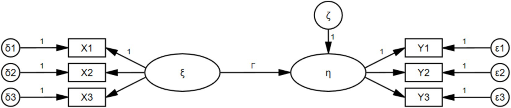
Figure 1. Example diagram of structural equation modeling (two-factor).

Every structural equation model has the following assumptions: (1) errors $\delta$ and $\epsilon$ are uncorrelated with latent variables, including exogenous and endogenous latent variables; (2) errors $\delta$ and $\epsilon$ are uncorrelated with each other; (3) errors $\zeta$ , $\delta$ , and $\epsilon$ are uncorrelated. Confirmatory factor analysis (CFA) is a special case of SEM that does not include the structural model, but only exogenous indicators and exogenous latent variables. Therefore, when modifying the model, it is necessary to follow the assumptions of uncorrelated errors $\delta$ and uncorrelated errors $\delta$ with latent variables. Although theoretically errors $\delta$ should not be correlated, due to systematic content biases of measurement tools (such as high similarity between exogenous indicators) or response biases of participants (such as practice effects), unexplained variations that cannot be accounted for theoretically may occur in different exogenous indicators, allowing for correlations between errors $\delta$ in such cases.

For general CFA models, correlations between errors $\delta$ cannot be established without reasonable explanations. However, there are some special CFA models that allow for correlations between errors $\delta$ , and sometimes this correlation is necessary.

The multitrait multimethod (MTMM) model measures multiple traits using multiple methods, aiming to test convergent validity, discriminant validity, and method effects. However, it is difficult to achieve the above validity or effect tests using the MTMM model. Therefore, the data from the MTMM model are often processed using factor analysis, where factors represent “traits” and “methods.” Scores of different traits measured by different methods belong to the same “trait” factor, and scores of different traits measured by the same method belong to the same “method” factor. This method is called correlated trait-correlated method (CTCM). Since the “traits” in the CTCM model are not measured by the same “method,” and the “traits” measured by the same “method” all have errors generated by that method, there may be correlations among the errors produced by different “methods.” For example, when two traits A and B are measured by two methods C and D, method C and method D may be affected by some common factors (such as the similarity of the evaluation environment, certain common behavioral characteristics of the evaluated objects, etc.), resulting in correlated errors. Therefore, the CTCM model allows correlations to be established among the error terms $\delta$ (Lance Charles et al., 2002).

The CTCM model of MTMM overcomes the challenges of validity testing. However, when the number of “methods” and “traits” is limited, the CTCM model may lead to non-convergence or results that cannot be positively defined, making it difficult to estimate the model. Marsh (1989) proposed the correlated trait-correlated uniqueness (CTCU) method to set factors. The CTCU model is based on the CTCM model, but it eliminates the “method” factor and only retains the “trait” factor. For scores obtained using the same method, it allows their errors $\delta$ to be correlated. Taking the CTCU model in Figure 2 as an example, the CTCU model in Figure 2 eliminates the method factor and only retains the trait factors $\xi 1$ and $\xi 2$ . If X1, X2, X5, and X6 are measured by the same method, and X3, X4, X7, and X8 are measured by the same method, then it is allowed to establish correlations among their errors.

Figure 2

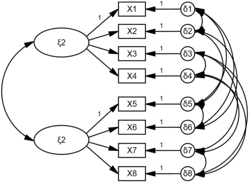
Figure 2. Example diagram of the CTCU model.

In most surveys and studies, due to limitations in manpower, financial resources, and material resources, cross-sectional studies are often conducted. The data from cross-sectional studies are collected at a specific point in time or within a relatively short time interval. Compared to cross-sectional studies, longitudinal studies can collect data on certain observational indicators at different time points. Since the data collected in longitudinal studies only involve changes over time and the observational indicators themselves do not change, it is generally believed that the error $\delta$ remains constant and unchanged between multiple data collection instances (Vandenberg and Lance, 2000), allowing for correlation to be established.

3 The core essence of model modification

The core of SEM analysis is the covariance matrix, which provides insights into the relationships between variables. Providing a covariance matrix with sufficient precision allows for the reproducibility of research results. There are three types of covariance matrices: sample, implied, and residual. The sample covariance matrix is derived directly from the sample data and serves as the original covariance matrix for SEM analysis. The implied covariance matrix is obtained by iteratively minimizing the difference between the sample covariance matrix and the hypothesized model. The residual covariance matrix is the difference between the sample and implied covariance matrices. SEM assesses the difference between the sample and implied covariance matrices using a chi-square test. Smaller differences suggest a better model fit, while larger differences indicate a poorer fit. Model evaluation is the preliminary step in model modification. Only a well-fitting model allows meaningful interpretation of SEM parameters (Wang et al., 2022). Unlike traditional statistics, SEM provides multiple model fit indices alongside p-values for a comprehensive fit evaluation. Upon passing the evaluation, the model proceeds to further analysis; otherwise, modifications are necessary.

3.1 Model fitness indicators and evaluation criteria

Since the emergence and popularity of structural equation modeling (SEM), scholars have proposed over 40 fit indices, which can be divided into three categories: absolute fit indices, relative fit indices (also known as incremental fit indices), and parsimony fit indices. Absolute fit indices include χ² (also known as CMIN), χ²/df, RMR, SRMR, RMSEA, etc. Relative fit indices include NFI, CFI, TLI, etc. Parsimony fit indices include PNFI, PCFI, PGFI, etc. Different fit indices represent the influence of different sample characteristics, and researchers can judge the model fit based on different indices. Due to the existence of numerous fit indices, careful consideration is needed when selecting which fit indices to evaluate the model. Some foreign scholars found through a study of 194 CFA studies published in American Association journals from 1998 to 2006 that almost all authors reported χ². Apart from χ², the most common fit indices were CFI (78.4%), RMSEA (64.9%), and TLI (46.4%) (Jackson et al., 2009). Currently, the recommended fit indices recognized by domestic scholars in China include CFI, TLI, RMSEA, and SRMR. A comparison reveals that the recommended fit indices by domestic and foreign scholars are almost the same. Regarding the recommended fit indices mentioned above, it is generally suggested that CFI and TLI should be >0.9 (Bentler and Bonett, 1980), and SRMR and RMSEA should be <0.08 (Browne and Cudeck, 1992) for the model to be considered acceptable. Other scholars believe that CFI and TLI should be >0.95, and SRMR and RMSEA should be <0.05 (Hu and Bentler, 1999) to be considered as excellent model fit standards. Moreover, the Gamma Hat is highly sensitive to model specification errors. It is an ideal indicator of model fit (Fan and Sivo, 2007) and also a commonly used one. Its value needs to be close to above 0.95 to indicate a good model fit (Li‐tze and Peter, 1999). The ratio of chi-square to degrees of freedom, compared with other commonly used fit indices, can effectively reflect the changes in the relationship between the model and the data caused by an increase in sample size (Herbert et al., 2004). Among the aforementioned fit indices, χ² is more susceptible to sample size. A larger sample size makes the chi-square test more likely to be significant (p < 0.05), thus indicating a poorer fit between the model and the sample data. A smaller χ² value is preferred, but there is no universally recognized standard for how small it should be to be considered good or how large it should be to be considered poor. Since χ² serves as the basis for calculating many other fit indices, most SEM analyses will present χ². The significant critical value of chi-square is 3.84. When it exceeds 3.84, it indicates that the model cannot be fitted to the data.

Each goodness-of-fit indicator can only judge the goodness of fit of a model from a certain perspective, and has its limitations. In addition, goodness-of-fit indicators are generally more or less influenced by factors such as sample size, data distribution, and parameter estimation methods (Shi and Maydeu-Olivares, 2020). Therefore, besides the aforementioned goodness-of-fit indicators, it is necessary to refer to other basic criteria. For example, whether the factor loading coefficient is significant and whether the standardized factor loading coefficient exceeds 0.7, whether the average variance extracted (AVE) reaches above 0.5, whether the composite reliability (CR) is above 0.5 (Kline, 1998), however, the Average Variance Extracted (AVE) test is often difficult to pass. In contrast, the Heterotrait-Monotrait Ratio (HTMT) test is not as stringent and serves as a better indicator. Under normal circumstances, when the value of HTMT reaches 0.85 (Clark and Watson, 1995) or 0.9 (Gold et al., 2001), it indicates that the model has good discriminant validity.Whether the correlation coefficients between factors are <0.85 or not (Kenny, 2016), and whether the variance and standard error are >0. In conclusion, it is important to scientifically and reasonably evaluate the goodness of fit of a model from multiple perspectives.

3.2 Modification indices and residual covariance matrix

The modification indices and standardized residual covariance matrix can be referred to for model Modification, which can be obtained from SEM analysis software such as Amos, LISREL, Mplus, etc.

Modification Indices (MI) refer to the reduction in the overall model chi-square (χ²) when a constrained parameter (usually fixed at 0) is freely estimated with one degree of freedom (df). This is achieved by changing the relationships between variables to improve the model fit. For example, if variables A and B are originally uncorrelated (correlation coefficient = 0), and the modification index is 10, then establishing a correlation between e1 and e2 through their free estimation will reduce the model’s χ² by 10 (with a decrease of 1 degree of freedom). Typically, when α is set to 0.05, the critical value of significant χ² for one degree of freedom is 3.84. If the modification index is <3.84, it indicates that there is no significant difference between the model before and after modification, and changing the parameters will not significantly improve the model fit. If the modification index is >3.84, it indicates that there is a significant difference between the model before and after modification, and changing the parameters will significantly improve the model fit.

The residual covariance matrix is obtained by subtracting the latent covariance matrix from the sample covariance matrix, and its elements are residual covariances. A positive residual covariance indicates that the sample covariance is greater than the latent covariance, and the model parameters underestimate the correlation between variables in the sample data. A negative residual covariance indicates that the sample covariance is smaller than the latent covariance, and the model parameters overestimate the correlation between variables in the sample data. For example, if the sample covariance between variables A and B is 0.6 and the latent covariance is 0.4, then the residual covariance is 0.2, indicating that the model should allow for a stronger direct or indirect path between variables A and B to match the higher correlation between A and B in the sample data. If the residual covariance between A and B is negative, it indicates that the model should reduce the direct or indirect paths to weaken the correlation between A and B in the sample data. Since residuals are influenced by the measurement units of variables, it is difficult to compare and measure them directly. Standardized residuals can be obtained by dividing the residuals by the square root of their estimated asymptotic variances, which are less affected by measurement units. They can serve as a standard for assessing model fit. If the absolute value of a standardized residual is >1.96 (p < 0.05), it indicates a significant difference between the variable relationships in the sample covariance matrix and the latent covariance matrix. In a well-fitting model, the majority of standardized residual covariances should be smaller than 1.96.

3.3 Parameters and strategies for model modification

There are three types of parameters to be adjusted: “Covariance,” “Variance,” and “Regression Weight.” For CFA, “Covariance” establishes the correlation between errors ( $\delta$ ) or errors ( $\delta$ ) and factors. “Variance” is used to check if the model’s variance has inappropriate values, such as if the value of error ( $\delta$ ) is too large or if both the factors and the variance of error ( $\delta$ ) are >0. In most cases, there is no need to adjust “Variance.” “Regression Weight” establishes the causal relationship between factors and observed indicators or between observed indicators. Cross-loadings refer to the causal relationship between factors and non-corresponding observed indicators, while establishing causal relationships between observed indicators is not desirable. In addition, if there are factor loading coefficients that are not significant (p > 0.05) or standardized factor loading coefficients that are <0.45, the corresponding observed indicators can be directly deleted. If multiple Modification indices with large values occur simultaneously, they should be adjusted in order of magnitude, and only one parameter can be adjusted at a time, followed by re-estimation of the model. If the model cannot be adjusted successfully at once, repeat the process until the model fits well.

Whether it is establishing correlations between errors ( $\delta$ ) or deleting measurement indicators, it is necessary to ensure that the model is identifiable. Model identification is a function of the number of distinct sample moments and the number of distinct parameters, i.e., whether the covariance matrix can provide sufficient information to estimate the free parameters.The calculation formula for the number of different sample moments is: $\frac{k\left(k+1\right)}{2}$ , k represents the number of observation indicators. The criteria for estimating the degrees of freedom for structural equation modeling (SEM) are as follows (Bishop, 2008): (1) The variances of all exogenous variables, including the error terms $\delta$ , $\epsilon$ , $\zeta$ , and the variances of exogenous latent variables. (2) The covariances between all exogenous variables. (3) The factor loading coefficients of all measurement indicators. Each latent variable’s latent scale needs to be specified, usually fixed at 1. This is because the loading coefficient will change with the change of the measurement unit of the latent variable. Without such a setting, any model would be unidentifiable. Factor loading coefficients that are fixed at 1 do not need to be estimated. (4) The regression coefficients between all measurement indicators or latent variables. (5) The variances and covariances of endogenous variables, as well as the covariances between exogenous variables and endogenous variables, are not parameters to be estimated by the model. The prerequisite for successful model identification is that the number of moment conditions from different sample moments should be greater than or equal to the number of free parameters estimated by the model, i.e., df ≥ 0. For a single-factor model, at least 3 measurement indicators are required for identification. For models with two or more factors, each factor should have at least 2 measurement indicators (Bollen and Davis, 2009). If a factor has only one indicator, it is not possible to simultaneously estimate the factor loading coefficients and the error term $\delta$ unless a method model fixes the factor loading coefficients and error term as fixes parameters and sets the factor variance as a free parameter.

4 Path for model modification methods

We estimated and modified the reading ability model shown in Figure 3 using AMOS software as the analysis tool (Xiong, 2023). The model includes four factors: Reading Perception Ability (RPA) with observed indicators RPA1 to RPA5, Understand Analytical Ability (UAA) with observed indicators UAA1 to UAA5, Appreciation Evaluation Ability (AEA) with observed indicators AEA1 to AEA4, and Creative Imagination Ability (CIA) with observed indicators CIA1 to CIA4. In total, the model comprises 18 observed indicators. The variables in this study are ordinal variables with a scale of 1 to 4. If the ordinal variables are treated as continuous variables, maximum likelihood estimation or weighted least squares estimation would be preferable analytical methods (Robitzsch, 2020). ML is the default estimation method in SEM analysis software. For this study, we utilized the software’s default ML method to estimate the model.

Figure 3

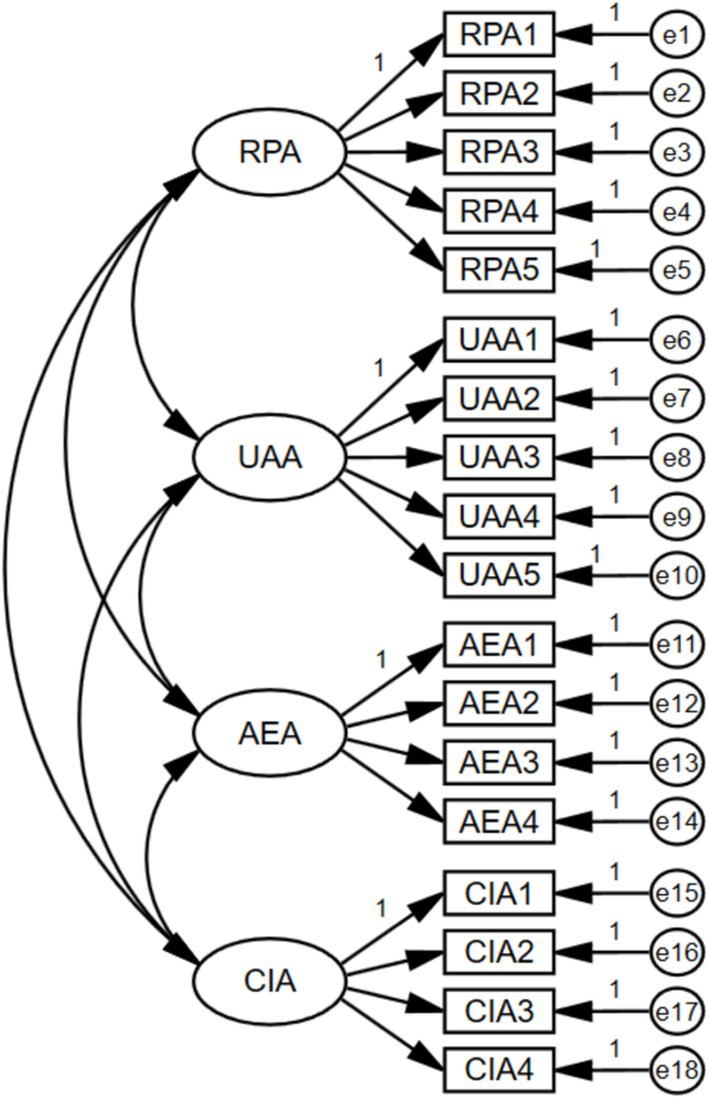
Figure 3. Confirmatory factor analysis.

The fit indices of the original model are shown in Table 1. The value of χ²/df is 3.4616, which falls within the lenient range of 3–5 but exceeds the stricter limit of 3. The values of TLI and CFI are 0.8810 and 0.8997, respectively, both below the acceptable criterion of 0.9. The values of SRMR and RMSEA are 0.0668 and 0.0800, respectively, both exceeding the criterion of 0.05. The AVE of one factor is 0.4810, while the other three factors are all above 0.5, indicating good overall convergent validity for most factors. The CR of all factors is above 0.5, indicating good composite reliability. Based on the fit indices mentioned above, it is evident that the model needs to be revised to achieve better fit.

Table 1

Table 1. Indicators of the original model fitting degree.

The study adopted three Modification methods, namely “deletion of observed indicators” “establishment of correlation (covariance)” and “a combination of both” to correct the model. The final models after applying these three Modification methods are named Model A, Model B, and Model C, respectively. The goodness-of-fit indicators of Model A, Model B, Model C, and the initial model all meet the standard. The process of Modification in the model is intended only as a demonstration and exploration of the methodology, without considering the actual interpretation of the model. To highlight the impact of Modification methods on the goodness-of-fit indicators, only the model χ² after each Modification is presented.

4.1 Model modification method 1: Removal of measurement indicators

As shown in Table 2, Model Modification Method 1 uses the method of deleting observed indicators for operation. The specific operation method is as follows: (1) Find the variable with the largest “M.I.” sequentially. (2) If there is a correlation between errors, compare the standardized factor loading coefficients of the corresponding observed indicators for the errors and examine the correlation between the two errors and other variables. For example, e3 and e2: if e3 needs to establish a correlation not only with e2 but also with many other variables, then delete the observed indicator corresponding to e3; otherwise, delete the observed indicator corresponding to e2. (3) If there is a correlation between errors and factors, directly delete the observed indicator corresponding to the error. (4) In multi-factor CFA, each factor should have at least one observed indicator. In summary, the model was modified a total of four times, deleting the observed variables “RPA2,” “CIA1,” “UAA1,” and “RPA4.” The final modified model’s chi-square value is 172.3445, which is lower than the initial model’s χ² by 274.2079.

Table 2

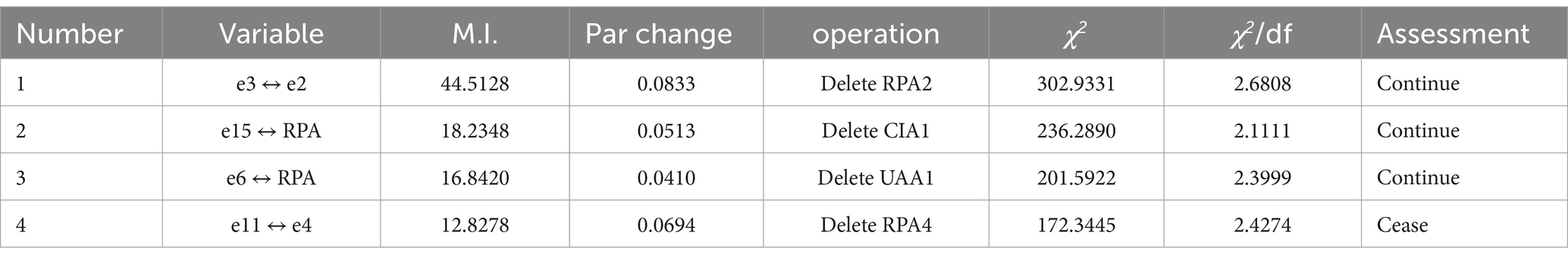
Table 2. Operational procedure for modification method 1.

The goodness-of-fit indices for Model A are shown in Table 3. The value of χ²/df is 2.4274, which falls within the range of 1 to 3. The values of TLI and CFI are 0.9419 and 0.9546, respectively, both exceeding the criterion of 0.9. The SRMR value is 0.0424, meeting the criterion of 0.05. The RMSEA value is 0.0615, complying with the lenient criterion of 0.08. Except for one factor with an AVE of 0.4791, all other factors have AVE values above 0.5, and the CR values for all factors are above 0.5. The model demonstrates good convergent validity and composite reliability. In conclusion, all the goodness-of-fit indices for the revised Model A meet the criteria for a well-fitting model.

Table 3

Table 3. Fit indices for model A.

The HTMT values of Model A are presented in Table 4. All the HTMT values are <0.85, indicating that there is a good degree of discriminant validity among the factors. Thus, Model A has good discriminant validity.

Table 4

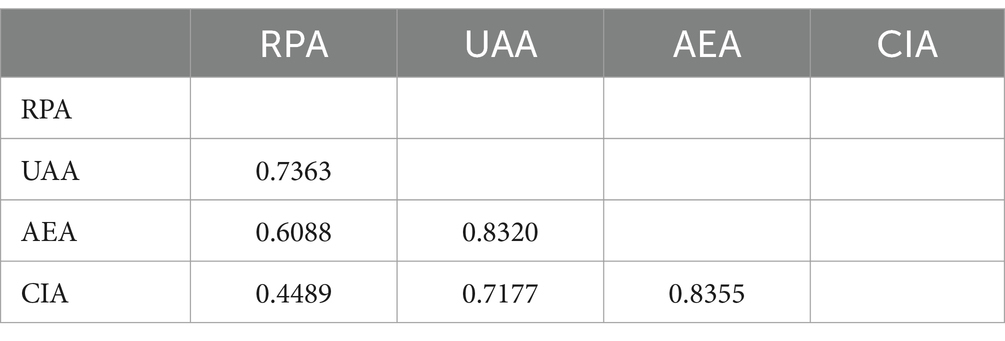
Table 4. HTMT for model A.

4.2 Model modification method 2: Establishing relevance

As shown in Table 5, Model Modification Method 2 uses a method based on establishing variable correlations for operation. The specific operational steps are as follows: sequentially identify the variables with the highest “M.I.” values that require establishing correlations and establish a correlation relationship between the two variables. The model was corrected a total of 6 times, establishing correlations between errors and between errors and factors. The final corrected model, χ² is 261.5837, which is 184.9687 lower than the initial model’s χ².

Table 5

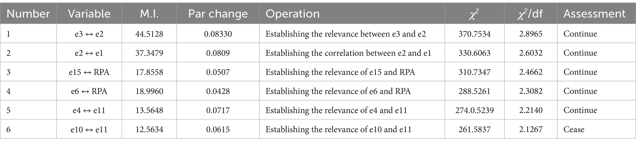
Table 5. Operational procedure for modification method 2.

The fit indices of Model B are shown in Table 6. The value of χ²/df is 2.1267, which falls within the range of 1 to 3. The values of TLI and CFI are 0.9455 and 0.9562, respectively, both higher than the criterion of 0.9. The value of SRMR is 0.0421, meeting the criterion of 0.05. The value of RMSEA is 0.0547, meeting the lenient criterion of 0.08. Except for one factor with an AVE of 0.4315, all other factors have values above 0.5. The CR values of all factors are above 0.5. The modified Model B demonstrates good convergent validity and composite reliability. In conclusion, all the fit indices of the modified Model B meet the criteria for a well-fitting model.

Table 6

Table 6. Goodness-of-fit indices for model B.

The HTMT values of Model B are shown in Table 7. There are some HTMT values exceeding 0.85, indicating that the discriminant validity among factors needs to be improved and that Model A may have poor discriminant validity.

Table 7

Table 7. HTMT for model B.

4.3 Model modification method 3: Deletion of observational indicators and establishment of relevance

As shown in Table 8, Model Modification Method 3 uses a combination of deleting observed indicators and establishing variable correlations for operations. The specific operation methods are as follows: (1) Find the variable with the largest “M.I.” value one by one. (2) If there is a correlation between the error and the factor, first consider deleting the observed indicator corresponding to the error. If the standardized factor loading coefficient of the deleted observed indicator is large, then consider establishing a correlation. (3) If there is a correlation between errors and the two correlated errors are less related to other variables, first consider establishing a correlation; otherwise, delete the observed indicators corresponding to the error variables that are more related to other variables. The model has been modified a total of four times, including establishing correlations between errors and deleting observed indicators. The final modified model chi-square is 188.4007, which is reduced by 258.1517 compared to the initial model.

Table 8

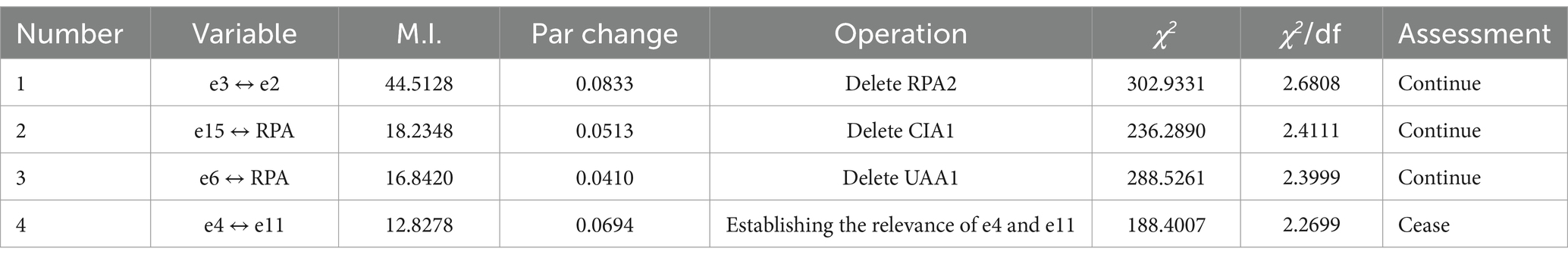
Table 8. Operational procedure for modification method 3.

The goodness-of-fit indices of Model C are shown in Table 9. The value of χ²/df is 2.2699, which falls within the range of 1 to 3. The values of TLI and CFI are 0.9444 and 0.9561, respectively, both higher than the criterion of 0.9. The value of SRMR is 0.0417, meeting the criterion of 0.05. The value of RMSEA is 0.0580, which satisfies the lenient criterion of 0.08. Except for one factor with an AVE of 0.4569, all other factors have values above 0.5, and the CR values of all factors are above 0.7. The model demonstrates good convergent validity and composite reliability. In conclusion, all the fit indices of the modified Model C meet the criteria for a well-fitting model.

Table 9

Table 9. Goodness-of-fit indices for model C.

The HTMT values of Model C are presented in Table 10. All the HTMT values are <0.85, indicating that there is a good degree of discriminant validity among the factors. Similarly, Model A also demonstrates good discriminant validity.

Table 10

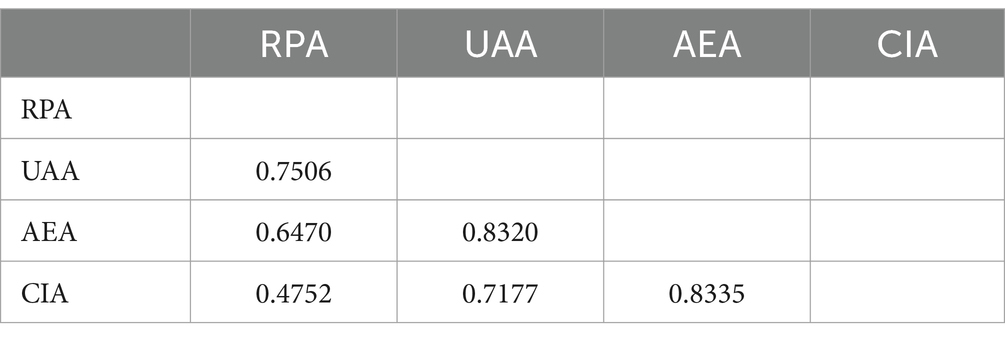
Table 10. HTMT for model C.

5 Discussion

5.1 The best way to modify the model is to delete the observed indicators

Through a detailed analysis of the modification process, frequency, and results mentioned above, it can be observed that in the first modification, both Modification Method 1 and Modification Method 3 used the approach of “deleting RPA2 corresponding to e2 to modify the model”. The chi-square value decreased from 446.5524 in the initial model to 302.9331, with a decrease of 143.6193. Modification Method 2, on the other hand, used the approach of “establishing a correlation between e3 and e2” in the first modification, resulting in a chi-square value decrease from 446.5524 in the initial model to 370.7534, with a decrease of 75.799.

It can be seen that compared to the modification approach of “establishing correlations between variables,” the modification approach of “deleting observed indicators” leads to a greater decrease in the chi-square value. This is because the modification approach of “establishing correlations between variables” only addresses the issue of chi-square value inflation caused by the lack of correlation between two variables in the model, while the modification approach of “deleting observed indicators” addresses the issue of chi-square value inflation caused by the lack of correlation between multiple variables. For example, after “deleting RPA2 corresponding to e2,” the issue of chi-square value inflation caused by the lack of correlation between “e2” and “RPA2” in the model will also be resolved. Therefore, the modification approach of deleting observed indicators leads to a greater decrease in the chi-square value.

In terms of the number of modifications, Modification Method 1 and Modification Method 3 were modified four times, while Modification Method 2 was modified six times. The final model’s chi-square value for Modification Method 1 was 172.3445, for Modification Method 2 was 261.5837, and for Modification Method 3 was 180.4007. It can be observed that although Modification Method 1 and Modification Method 3 have the same number of modifications, which is four times, the reduction in the chi-square value of the modification method that completely adopts “deleting observed variables” is much greater than that of the combination of “deleting observed indicators” and “establishing correlations between variables.” In addition, in terms of other goodness-of-fit indices, Modification Method 1 is also the best among the three modification methods overall.

5.2 Model modification is a process of sequential adjustment, dynamic change, and comprehensive judgment

The differences in each revision method can also lead to changes in subsequent revision methods. For example, in Revision Method 1 and Revision Method 3, the first revision involves “deleting RPA2 corresponding to e2,” while their second revision involves “deleting CIA1 corresponding to e15.” Revision Method 2, on the other hand, revises the model by first establishing the correlation between e3 and e2, and then, in the second revision, establishing the correlation between e2 and e1. Therefore, it is best to revise one parameter at a time during model revision and decide the next revision method based on the revised results. The Mutual Information (MI) provided by the software is merely a mathematical result of association and equations, similar to χ². MI is also influenced by the sample size, so model revision cannot rely solely on MI. In addition, the model fit index is an empirical judgment agreed upon by scholars. When to stop revising the model should not be determined only by the fit index but also requires researchers to examine the model’s significance from a professional and theoretical standpoint.

5.3 Model modification should be supported by theoretical evidence and cross validation should be conducted after the modification

When researchers adjust a model, they should carefully consider relevant theories and understand which modifications are feasible and which ones contradict assumptions, logic, and so on. It is crucial not to ignore the practical significance of the model itself. For example, the most commonly used and reasonable way to improve the goodness-of-fit index in actual model adjustments is through modification method 1, which removes measurement indicators. On the other hand, modification method 2, which suggests establishing correlations between measurement errors, requires theoretical support. However, establishing correlations between measurement errors and factors contradicts assumptions and logic. Mathematically driven modification methods are not desirable as they may lead to a “data-driven” pitfall. Even if a highly fitting model is obtained in the end, it might lack value or meaning. Furthermore, while confirmatory factor analysis (CFA) originally aims to validate the quality of a model using collected sample data, model adjustments involve an ongoing exploration for the best model, thus deviating from the essence of CFA. Although the adjusted model may have a good fit with the sample data, it could significantly differ from the original hypothesized model. Therefore, some scholars suggest that it is necessary to cross-validate the model and use the cross-validity fit index to verify the model’s cross-validity (Browne and Cudeck, 1989). If the sample size is large, the sample data can be randomly divided into two subsets, one for exploring the model and the other for validating the model; if the sample is small, additional data can be collected for validation. In conclusion, separately estimating and correcting the measurement model is an important step in the “two-step approach” to structural equation modeling, which should take into account the theory and content, residual matrix, factor loading coefficients, and other information to make a comprehensive judgment on the poorly fitted model by removing or adding indicators, and establishing correlations between errors, to ensure the model fit and interpretability (Anderson and Gerbing, 1988). Furthermore, if relatively large values appear in the modification indices of CFA regarding error correlations, it may indicate the presence of common method biases caused by factors such as the same data source, raters, or measurement environment. Statistical methods can be employed to test and control for common method biases. For instance, Harman’s single-factor test can determine whether common method biases exist. If they do, the “latent method factor control” can be utilized, adding a method factor to explain variance and thus improve the model’s fit indices.

Data availability statement

The raw data supporting the conclusions of this article will be made available by the authors, without undue reservation.

Author contributions

ZX: Writing – original draft, Writing – review & editing. HX: Writing – review & editing, Conceptualization, Investigation, Resources. JN: Writing – review & editing, Methodology, Funding acquisition. HH: Writing – review & editing, Supervision, Project administration, Validation.

Funding

The author(s) declare that financial support was received for the research, authorship, and/or publication of this article. This research was funded by the National Social Science Fund, with the project number 20BKS129. The fund supported various aspects such as data collection and field investigations, which significantly contributed to the smooth progress of the research.

Conflict of interest

The authors declare that the research was conducted in the absence of any commercial or financial relationships that could be construed as a potential conflict of interest.

Generative AI statement

The author(s) declare that no Generative AI was used in the creation of this manuscript.

Publisher’s note

All claims expressed in this article are solely those of the authors and do not necessarily represent those of their affiliated organizations, or those of the publisher, the editors and the reviewers. Any product that may be evaluated in this article, or claim that may be made by its manufacturer, is not guaranteed or endorsed by the publisher.

Supplementary material

The Supplementary material for this article can be found online at: https://www.frontiersin.org/articles/10.3389/feduc.2025.1506415/full#supplementary-material

References

Anderson, J. C., and Gerbing, W. (1988). Structural equation modeling in practice: a review and recommended two-step approach. Psychol. Bull. 103, 411–423. doi: 10.1037/0033-2909.103.3.411

Crossref Full Text | Google Scholar

Bentler, P. M., and Bonett, D. G. (1980). Significance tests and goodness of fit in the analysis of covariance structures. Psychol. Bull. 88, 588–606. doi: 10.1037/0033-2909.88.3.588

Crossref Full Text | Google Scholar

Bishop, J. W. (2008). A first course in structural equation modeling. Organ. Res. Methods 11, 408–411. doi: 10.1177/1094428107308985

Crossref Full Text | Google Scholar

Bollen, K. A., and Davis, W. R. (2009). Two rules of identification for structural equation models. Struct. Equ. Model. 16, 523–536. doi: 10.1080/10705510903008261

Crossref Full Text | Google Scholar

Browne, M. W., and Cudeck, R. (1989). Single sample cross-validation indices for covariance structures. Multivar. Behav. Res. 24, 445–455. doi: 10.1207/s15327906mbr2404_4

PubMed Abstract | Crossref Full Text | Google Scholar

Browne, M. W., and Cudeck, R. (1992). Alternative ways of assessing model fit. Sociol. Methods Res. 21, 230–258. doi: 10.1177/0049124192021002005

Crossref Full Text | Google Scholar

Cao, X. (2023). The application of structural equation model in psychological research. CNS Spectr. 22, S17–S19. doi: 10.1017/S1092852923000858

Crossref Full Text | Google Scholar

Clark, L. A., and Watson, D. (1995). Constructing validity: basic issues in objective scale development. Psychol. Assess. 7, 309–319. doi: 10.1037/1040-3590.7.3.309

Crossref Full Text | Google Scholar

Fan, X., and Sivo, S. A. (2007). Sensitivity of fit indices to model misspecification and model types. Multivar. Behav. Res. 3, 509–529. doi: 10.1080/00273170701382864

Crossref Full Text | Google Scholar

Gold, A. H., Malhotra, A., and Segars, A. H. (2001). Knowledge management: an organizational capabilities perspective. J. Manag. Inf. Syst. 18, 185–214. doi: 10.1080/07421222.2001.11045669

Crossref Full Text | Google Scholar

Herbert, W. M., Kit-Tai, H., and Zhonglin, W. (2004). In Search of Golden Rules: Comment on Hypothesis-Testing Approaches to Setting Cutoff Values for Fit Indexes and Dangers in Overgeneralizing Hu and Bentler’s (1999) Struct Equ Modeling. 3, 320–341. doi: 10.1207/s15328007sem1103_2

Crossref Full Text | Google Scholar

Hou, J., and Cheng, Z. (1999). The application and analysis strategy of structural equation modeling. Psychol. Explor. 1, 54–59. doi: 10.3969/j.issn.1003-5184.1999.01.010

Crossref Full Text | Google Scholar

Hu, L., and Bentler, P. M. (1999). Cutoff criteria for fit indexes in covariance structure analysis: conventional criteria versus. Struct. Equ. Model. 6, 1–55. doi: 10.1080/10705519909540118

Crossref Full Text | Google Scholar

Hu, P., Lu, H., and Ma, Z. (2018). The feasibility and conditionality of allowing error correlation in confirmatory factor analysis. Statistics Decision 19, 37–41. doi: 10.13546/j.cnki.tjyjc.2018.19.008

Crossref Full Text | Google Scholar

Jackson, D. L., Gillaspy, J. A. Jr., and Purc-Stephenson, R. (2009). Reporting practices in confirmatory factor analysis: an overview and some recommendations. Psychol. Methods 14, 6–23. doi: 10.1037/a0014694

PubMed Abstract | Crossref Full Text | Google Scholar

Kenny, D. A. (2016). Multiple latent variable models: confirmatory factor analysis. Available at: https://davidakenny.net/cm/mfactor.htm (Accessed April 13, 2016).

Google Scholar

Kline, R. B. (1998). Software review: software programs for structural equation modeling: Amos, eqs, and lisrel. J. Psychoeduc. Assess. 16, 343–364. doi: 10.1177/073428299801600407

Crossref Full Text | Google Scholar

Lance Charles, E., Noble Carrie, L., and Scullen, S. E. (2002). A critique of the correlated trait-correlated method and correlated uniqueness models for multitrait-multimethod data. Psychol. Methods 7, 228–244. doi: 10.1037/1082-989X.7.2.228

Crossref Full Text | Google Scholar

Li‐tze, H., and Peter, M. B. (1999). Cutoff criteria for fit indexes in covariance structure analysis: Conventional criteria versus new alternatives, Structural Equation Modeling: A Multidisciplinary Journal. 1, 1–55.

Google Scholar

MacCallum, R. C., and Austin, J. T. (2000). Applications of structural equation modeling in psychological research. Annu. Rev. Psychol. 51, 201–226. doi: 10.1146/annurev.psych.51.1.201

Crossref Full Text | Google Scholar

Marsh, H. W. (1989). Confirmatory factor analyses of multitrait-multimethod data: many problems and a few solutions. Appl. Psychol. Meas. 13, 335–361. doi: 10.1177/014662168901300402

Crossref Full Text | Google Scholar

Michael, E. S. (1992). Review:the American occupational structure and structural equation modeling in sociology. Contemp. Sociol. 21, 662–666. doi: 10.2307/2075551

Crossref Full Text | Google Scholar

Robitzsch, A. (2020). Why ordinal variables can (almost) always be treated as continuous variables: clarifying assumptions of robust continuous and ordinal factor analysis estimation. Methods 5:589965. doi: 10.31234/osf.io/hgz9m

Crossref Full Text | Google Scholar

Shi, D., and Maydeu-Olivares, A. (2020). The effect of estimation methods on SEM fit indices. Educ. Psychol. Measur. 80, 421–445. doi: 10.1177/0013164419885164

PubMed Abstract | Crossref Full Text | Google Scholar

Teegan, G. (2016). A methodological review of structural equation modelling in higher education research. Stud. High. Educ. 12, 2125–2155. doi: 10.1080/03075079.2015.1021670

Crossref Full Text | Google Scholar

Vandenberg, R. J., and Lance, C. E. (2000). A review and synthesis of the measurement invariance literature: suggestions, practices, and recommendations for organizational research. Organ. Res. Methods 3, 4–70. doi: 10.1177/109442810031002

Crossref Full Text | Google Scholar

Wang, X., and Qu, L. (2020). A review of structural equation modeling and its application in the economic field. Modern Bus. 27, 23–25. doi: 10.14097/j.cnki.5392/2020.27.009

Crossref Full Text | Google Scholar

Wang, Y., Wen, Z., Li, W., and Fang, J. (2022). Domestic research and model development of structural equation modeling in the past 20 years of the new century. Adv. Psychol. Sci. 30, 1715–1733. doi: 10.3724/SP.J.1042.2022.01715

PubMed Abstract | Crossref Full Text | Google Scholar

Xiong, Z. (2023). The development of a Reading ability scale for junior high school students in Chinese and its application in evaluation [Master's Degree Thesis]. Zhoushan: Zhejiang Ocean University.

Google Scholar