 Martin Abt
 Timo Leuders
 Katharina Loibl
 Anselm R. Strohmaier
 Wim Van Dooren4
 Frank Reinhold
- 1Institute for Mathematics Education, University of Education Freiburg, Freiburg, Germany
- 2Institute of Psychology, University of Education Freiburg, Freiburg, Germany
- 3Institute of Mathematics II, University of Education Ludwigsburg, Ludwigsburg, Germany
- 4Centre for Instructional Psychology and Technology, University of Leuven, Leuven, Belgium
Tasks in which learners are asked to compare two data sets using box plots and decide which distribution contains more observations above a given threshold have already been investigated in research. There are indications that these tasks are solved schema-based and that different (correct and erroneous) schemas are used depending on the arrangement of the quartiles around the threshold. Erroneous schemas can cause systematic errors and are often based on typical misconceptions. For example, if learners did not complete the conceptual change and assume that in box plots – like in most other statistical representations (e.g., bar or circle diagrams) - more (box) area also represents more observations, they decide the task according to which box plot shows more box area above the threshold. However, this can lead to incorrect answers, as the box area does not represent frequency but the range of the middle half of the data (interquartile range) and thus a measure of variability. So far, these schema-based reasoning processes have mainly been investigated via differences in solution rates of congruent and incongruent items. The present study investigates whether eye-tracking data can help to better understand which information is processed in the different schemas. Our research interest is based on hypotheses specifying which box plot components are significantly involved in the different schemas. We assume that the gaze patterns of learners using different schemas differ both regarding the number and duration of fixations on the relevant box plot components (areas of interest) and in terms of the number of transitions between them. We asked N = 14 participants to solve congruent and incongruent items and simultaneously collected eye movement data. In the analysis, we first used the solution rates to assign the schemas most likely used. Subsequently, the eye-tracking data were analyzed regarding differences in line with our hypotheses. We found hypothesis-compliant effects in all schemas regarding the number of fixations and transitions, but not regarding fixation duration. These results not only validate the schemas identified in previous studies, but also indicate that the schemas differ primarily in terms of which quartile is focused.
1 Introduction
1.1 Comparing data sets through box plots
In today’s digitalized and interconnected world, large amounts of data are collected and evaluated. In the public or political sphere, hardly any debate is carried out without referring to study results or statistical data to support one’s own position. Whether in the context of epidemics or global climate change, or even in everyday life situations people are often faced not only with the challenge of being able to assess empirically supported arguments, but also to make their own data-driven decisions. Therefore, statistical literacy has become an integral part of the school curriculum and, not least, mathematics education provides important tools for evaluating data in a reputable manner (Ben-Zvi et al., 2018; Garfield and Ben-Zvi, 2008; Watson, 2006). Among these tools, the box plot (Tukey, 1977) takes an important position (National Council of Teachers of Mathematics, 2000). However, box plots– frequently used in scientific contexts (Streit and Gehlenborg, 2014) – are a challenging topic to learn since they display a number of descriptive statistical parameters in a condensed form (Bakker et al., 2005; Behrens et al., 1990; Edwards et al., 2017; Finger and Spelt, 1947): Box plots represent the statistical distribution of one quantitative variable by dividing the distribution into four equally sized1 subsets and plotting the cut-offs (quartiles) as short vertical lines along a x-axis (Figure 1). While the smallest observation (minimum) and the first quartile as well as the third quartile and the largest observation (maximum) are each connected by a horizontal line (upper and lower whisker), the first and third quartiles form the lateral outlines of a box representing the middle half of the data. The second quartile (median) - within the box - splits the distribution into an upper and a lower half and is used as a robust central value (Dodge, 2008). However, the box plot can be understood not only as a four-part distribution, but also as an overlay of two measures of variability, − the range, i.e., the distance between the minimum and maximum, and the more robust interquartile range (IQR), i.e., the distance between the first and third quartiles, indicated by the width of the box. This simultaneous presence of measures of central tendency and variability is a unique feature of the box plot (Cobb and Moore, 1997) and makes it a suitable tool for comparing distributions at a glance (Kader and Perry, 1996; Krzywinski and Altman, 2014; Massart et al., 2005). From this perspective, the boxplot is particularly relevant for students in the middle grades. While pupils learn about central tendency from an early age and are familiar with measures of central tendency such as the arithmetic mean or the median, there is no corresponding routine in dealing with measures of variability (e.g., Reading and Shaughnessy, 2004). Often in higher grades, standard deviation is the first systematic exposure to the concept of variability although the interplay of variability and central tendency is considered the core of statistical science (Shaughnessy, 1997). The boxplot, which introduces the interquartile range as another quantile-based measure of variability in addition to the range, not only supports the acquisition of conceptual knowledge about variability, but also allows middle school students to compare distributions in a differentiated way, including a more robust measure of variability compared to the range. We argue that these two perspectives on box plots (four-part split of a distribution / overlay of measures of variability) are mirrored in two types of tasks that can be solved via box plots. As an example we assume the following functional context (Strohmaier et al., 2022) (referenced “school context” in the following): Two schools (A and B) are attended by the same number of children. At both schools, a survey was carried out in which all children answered the question of how many minutes it takes them to get to school in the morning (Figure 1).
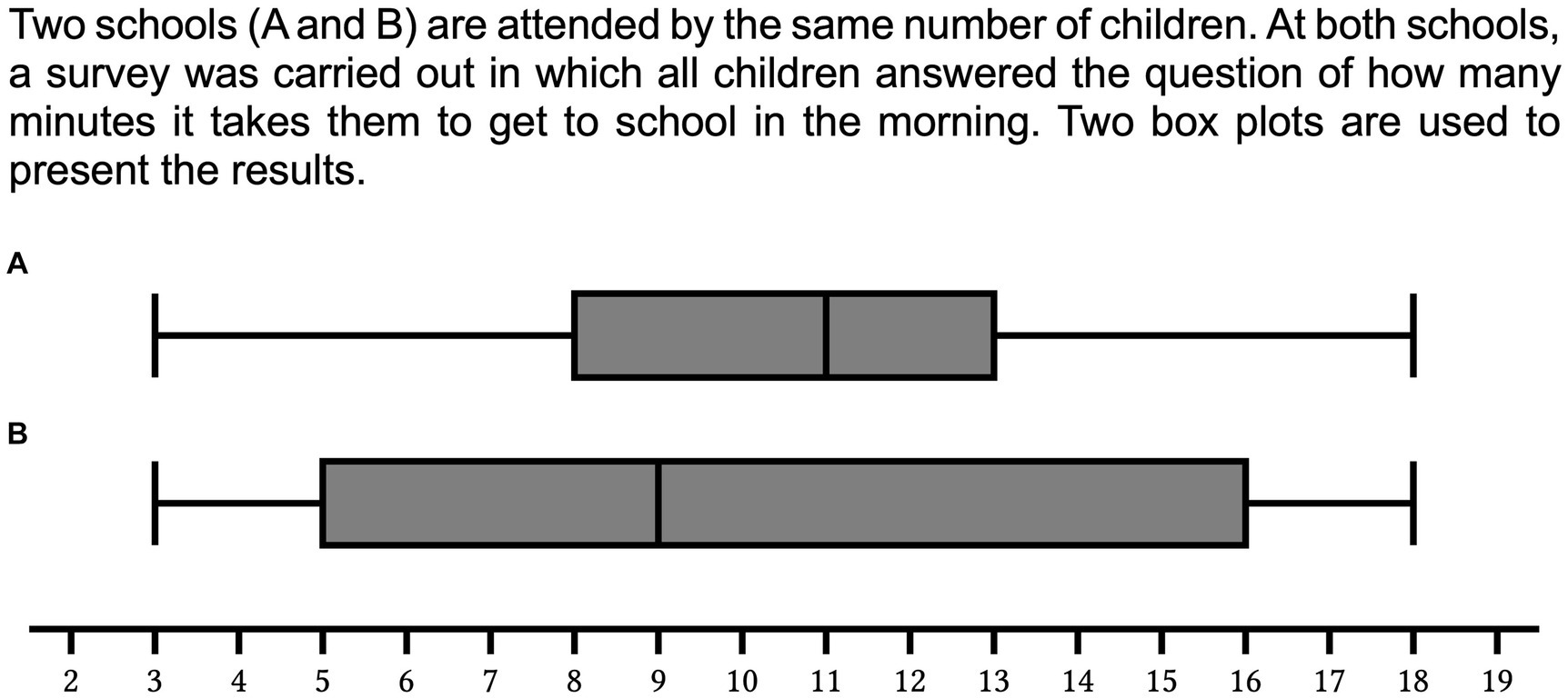
Figure 1. Two box plots representing five characteristic values of the represented distribution: the extremes values (minimum and maximum), the first and the third quartile and the median.
Within such functional contexts different task types of tasks are conceivable:
(1) In the first task type, a comparison of variability (here: distances between the quartiles) and not a comparison of absolute values is key to the solution. For the school context (Figure 1) a question that addresses variability would be: at which of the two schools do the children take a more similar amount of time to get to school in the morning (correct answer: school A, since box plot B shows a higher IQR than box plot A)?
(2) In a second task type, a comparison of the location parameters (minimum, maximum, first/third quartile, median) is key to the solution.
(a) One subtype are tasks that require focusing the highest and/or lowest value of a given proportion (e.g., the upper quarter) of a distribution. For the school context (Figure 1) a question would be: at which of the two schools do you have to spend longer walking to school in the morning to be among the 25% of children with the longest way to school (correct answer: school B, since in box plot B the third quartile is 16, whereas the third quartile in box plot A is only 13)?
(b) Another subtype require identifying the proportion of a distribution that is above or below one or two predefined threshold values. For the school context (Figure 1) a question would be: at which school there are more children who travel longer than 10 min (critical value) to school in the morning (correct answer: school A, since box plot A shows a median above the critical value)?
1.2 Systematic student errors in critical-value-comparison tasks
Type 2b tasks, which we also refer to as critical-value-comparison tasks thus represent one of three basic requirements that learners have to master when interpreting boxplots. This type of task has already been investigated in a number of studies (e.g., Abt et al., 2022, 2023, 2024; Lem et al., 2013). Two systematic student errors have been described that frequently lead to erroneous solutions: One particular hurdle when dealing with box plots is the correct interpretation of the box area (delMas, 2004). In many data representations like histograms or circle charts, areas are proportional to frequencies. In box plots, the box always represents half of the data, regardless of its area. Rather, the box area is proportional to the range of the middle half of the data and is therefore an indicator of variability (interquartile range, IQR). Learners may not fully manage this conceptual change (Posner et al., 1982; Vosniadou and Verschaffel, 2004) when learning about box plots and continue interpreting area as an indicator of frequency (area misconception) (Abt et al., 2022, 2023, 2024; Bakker et al., 2005; Lem et al., 2013). When students in critical-value-comparison tasks compare the area above the critical value to determine the correct solution, this can lead to errors.
In Figure 2A the item can be answered by comparing the medians since there is exactly one median above the critical value. Therefore, the correct answer is school A. However, if students are subject to the area misconception and think more area also represents a higher number of observations, they decide according to which box plots shows more area above the critical value of 10 min and will give the incorrect answer (school B). This systematic error was first systematically investigated by Lem et al. (2013). Central values are often introduced at an early stage and not just in the context of instruction on box plots. Thus, when students identify the median in the box plot representation then they might use this isolated knowledge even if a comprehensive conceptual about the box plot as a whole is not available. The prominent importance of central values for data-driven decisions was describes in a number of previous research (Biehler, 1997; Kramer et al., 2017; Masnick and Morris, 2008; Obrecht et al., 2007). Abt et al. (2022, 2023, 2024) therefore assumed that, in addition to area misconception as a cause of errors in critical-value-comparison tasks, an overgeneralization of the comparison of medians in tasks in which a comparison of medians is not an appropriate approach is another plausible cause of errors. In Figure 2B the correct solution can be determined by comparing the first quartiles since exactly one of the two first quartiles is located above the critical value. Therefore, the correct answer is school A. Contrary, comparing the medians and choosing the higher median leads to an incorrect solution (school B). Since both medians are above the critical value, they cannot be used to answer the question.
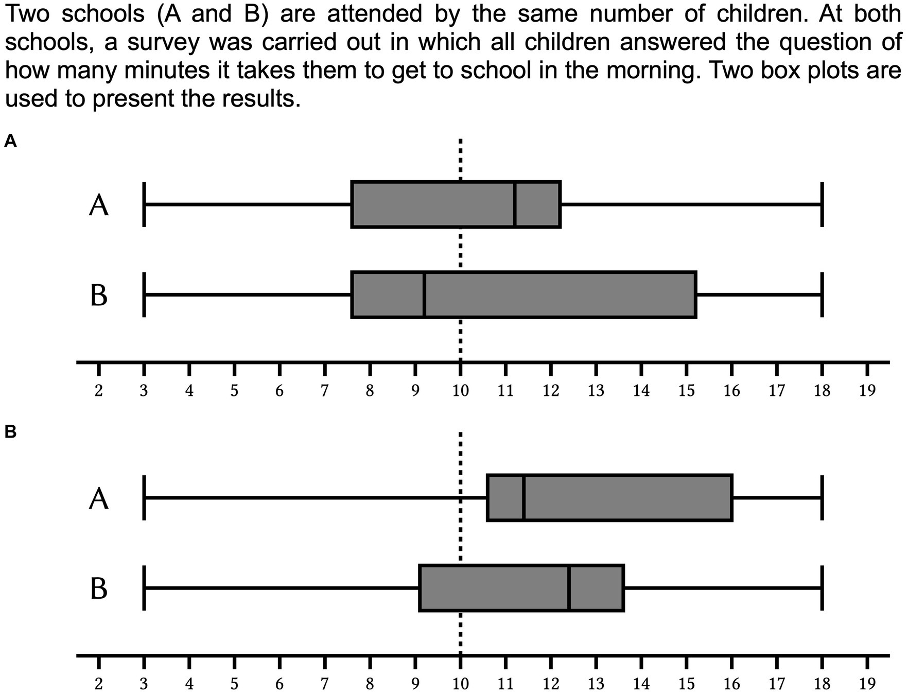
Figure 2. Two box plot pairs representing a comparison of how long students at school A/B spend getting to school in the morning. Box plot pair (A) can be solved by comparing the medians, box plot pair (B) can be solved by comparing the position of the boxes.
1.3 Detecting systematic errors via congruent and incongruent items
Abt et al. (2022, 2023, 2024) used congruent and incongruent items to identify these errors and to make predictions about whether students in critical-value-comparison tasks display one of these two systematic errors. The authors distinguished six different item categories (Figure 3): First, they distinguish two item types: In median items (Figure 3, first row) exactly one of the two box plots shows a median above the critical value. Therefore, median items can be solved by comparing the medians. In items (A) and (B) box plot A shows a median above the critical value. This indicates that more than half of the children attending school A have a walk to school of more than 10 min. In box plot B, on the other hand, the median is below the critical value, indicating that less than half of the children attending school B have a walk to school of more than 10 min. So, in both items school A is the correct answer. However, in item (A) comparing the area above the critical value leads to the correct answer (school A) as well. This is why the authors call this median item area congruent. Conversely, in item (B) comparing the area above the critical value leads to the incorrect answer (school B). This is why the authors call this median item area incongruent.
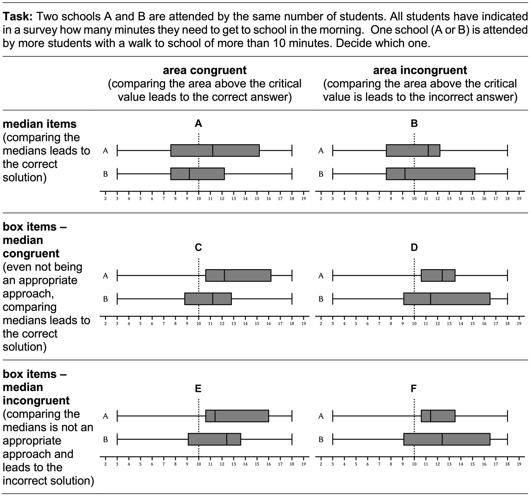
Figure 3. According to Abt et al. (2024) six item categories distinguish possible items according to item type (median items / box items) and two levels of congruency (area congruency /median congruency). Item (A) is an area congruent median item, item (B) is an area incongruent median item, item (C) is an area congruent, median congruent box item, item (D) is an area incongruent, median congruent box item, item (E) is an area congruent, median incongruent box item, and item (F) is an area incongruent and median incongruent box item.
In addition to median items, the authors consider items in which comparing the medians is not an appropriate approach, since both medians are above the critical value (Figure 3, second and third row). In the items (C) – (F) in exactly one of the two box plots the entire box lies above the critical value, e.g., comparing the position of the boxes can considered to be an appropriate approach. This is why the authors call such items box items. In all four box items, box plot A shows a box completely located above the critical value. This means that more than three quarters of the children attending school A have a walk to school of more than 10 min. Conversely, less than three quarters of the children attending school B have such a long walk. So, in all four items, school A is the correct answer. In items (C) and (E), comparing the area above the critical value leads to the correct answer. That is why those box items are called area congruent. Conversely, in items (D) and (F) comparing the area above the critical value leads to the incorrect answer. That is why those box items are called area incongruent. Even if a comparison of the medians in box items is always inappropriate, the comparison still leads to a correct answer in some cases. Analogous to the distinction between area congruent and area incongruent items, this results in a second level of congruence for box items, − the median congruency. Since in items (C) and (D) box plot A also shows the higher median, a comparison of the medians leads to the correct answer here. Such box items are therefore called median congruent. Conversely, in items (E) and (F) box plot B shows the higher median, so that a comparison of the medians here leads to the incorrect answer. Such box items are therefore called median incongruent.
These item categories can be used to identify systematic errors: If students compare the area above the critical value, this shows up in high solution rates, i.e., solution rates significantly above the guessing probability, in area congruent items, and in low solution rates, i.e., solution rates significantly below the guessing probability, in area incongruent items. If students compare the median even when this approach is not appropriate, this shows up in high solution rates, i.e., solution rates significantly above the guessing probability, in median congruent box items, and in low solution rates, i.e., solution rates significantly below the guessing probability, in median incongruent box items.
Abt et al. (2024) identified the characteristics item type (median items/box items), median congruency (median congruent/median incongruent), and area congruency (area congruent/area incongruent) as difficulty-generating item variables and found that over 80% of the variance of item solutions could be explained by these variables. The authors found that median items were more likely to be solved correctly than box items, median-congruent box items were more likely to be solved correctly than median-incongruent box items, and area-congruent items were more likely to be solved correctly than area-incongruent items. In addition, they were able to show at the person level that participants did not answer items correctly or incorrectly randomly, but that participants answered items belonging to one of the six item categories either consistently correctly or consistently incorrectly.
Taken these empirical results together, it seems highly plausible that the reason for the systematic differences in solution rates is that learners use different schemas (Chi et al., 1982; Mandler, 2014; Rumelhart et al., 1986) in critical-value-comparison tasks. In addition to a median schema (leading to correct answers in median items and median-congruent box items), Abt et al. (2024) assumed a box schema (leading to correct answers in box items) and an area schema (leading to correct answers only in area congruent items).
1.4 The present study
Even if the results of Abt et al. (2022, 2023, 2024) suggest that items for critical-value-comparison tasks are solved using different schemas that lead to correct or incorrect answers in different item categories, it remains unclear which components of the box plot are used in the decision-making process. In contrast to the median schema – where the only plausible type of decision making is the pairwise comparison of the median – it is not yet clear whether the box and the area schema also involve a pairwise comparison of quartiles. Students may perceive the box as a unit representing the middle half of the data. Thus, they may or may not answer the question of whether this box is above the critical mark via a pairwise comparison of the first quartiles (box schema). Similarly, they may or may not answer the question of which box plot shows more box area above the critical mark via a pairwise comparison of the third quartiles (area schema). How students answer these questions cannot be derived adequately via congruently and incongruently designed items. Therefore, Abt et al. (2023) used the terms box schema and area schema as (preliminary) umbrella terms without specifying exactly which boxplot components are involved in the decision-making process and in which way. This research question requires insight on how students relate the information (i.e., the components of the boxplot) to each other during the decision-making process. Assuming that eye movement data allow conclusions about such underlying cognitive processes (Holmqvist et al., 2011) eye-tracking methodology is an appropriate approach to quantitatively investigate and better understand the cognitive processes underlying box and area schema.
From an instructional perspective, insights into these decision-making processes are highly desirable for essentially two reasons: Firstly, understanding cognitive processing enables more targeted intervention during instruction on box plots. Secondly, numerous variations in the design of the boxplot (horizontal/vertical, shaded/unshaded box, thickness of the lines, etc.) have been described in the literature (e.g., Watson et al., 2008). We argue that such discussions on improving the box plot design can benefit from insights into the question of which box plot components are focused on in the context of certain questions and to what extent these focuses lead to correct and incorrect solutions.
Therefore, in the present study eye-tracking data was used to investigate the following research question: When we know a student’s solution rates in the different item categories, we already have a strong indication of which schema the student most likely applies in median and which schema the student most likely applies in box items. Will the corresponding gaze patterns in the eye-tracking data then (i) provide information about which box plot components are primarily focused on when applying different schemas, and (ii) substantially differ depending on the schema used.
The eye-mind-assumption behind this idea was initially formulated for the area of text comprehension (Just and Carpenter, 1980) and has since been part of the established repertoire of research on learning and instruction for years. Between 2000 and 2012, Lai et al. (2013) identified 113 studies that investigated learning processes using eye-tracking data. The authors were able to identify seven main areas in which eye movements were used to gain insight: patterns of information processing, effects of instructional design, reexamination of existing theories, individual differences, effects of learning strategies, conceptual development, and – as in the present paper – pattern of decision making. In addition to this cross-sectional spectrum of different possible applications, there is also an increasing number of domain-specific applications in the field of mathematical education (Lilienthal and Schindler, 2019; Strohmaier et al., 2020) and especially in the field of research on the interpretation of statistical graphs (e.g., Boels et al., 2019). For example, using eye-tracking data, Schreiter and Vogel (2023) were able to find empirical-quantitative evidence for the differentiation between a perception of a distribution as a set of individual data (local perspective) and a perception as a conceptual entity (global perspective), which had previously been assumed mainly on a theoretical level.
The fact that we triangulate the eye movement data with solution rates and interpret them together in our research design also takes into account that equating the visual and cognitive focus has proven to be problematic (Schindler and Lilienthal, 2019) and that the question of the relevance of the characteristic interweaving of text, symbols, and visualizations in mathematics is unclear (Andrà et al., 2009; Ott et al., 2018). To draw conclusions about which areas of the box plots are compared, we use three established measures: The fixation duration (on one or more areas of interest, AOIs), the number of fixation (on one or more AOIs) and the number of transitions (between two AOIs) (Holmqvist et al., 2011).
1.4.1 Median schema
We assume that the median schema is a pairwise comparison of the medians and that eye-tracking data support this focus from three (quantitative) perspectives (Figure 4A).
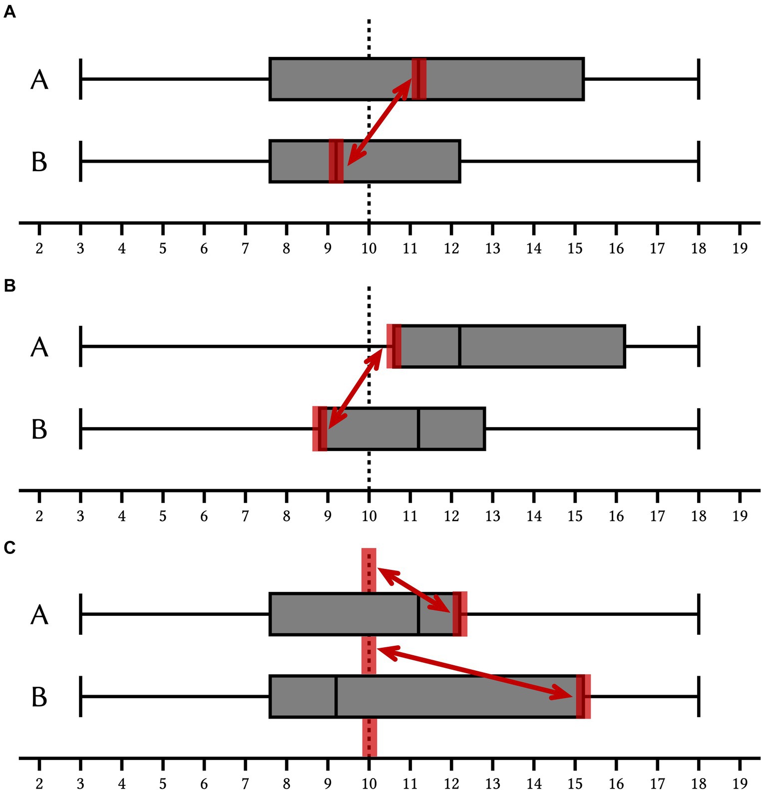
Figure 4. Illustration of the hypotheses regarding the median schema (A), the box schema (B), and the area schema (C). The critical value is indicated as a dashed line.
H1a: [longer fixation duration] Students who can be considered to systematically apply the median schema show a longer fixation duration on the medians than those who cannot be considered to systematically apply the median schema.
H1b: [higher number of fixations] Students who can be considered to systematically apply the median schema show a higher number of fixations on the medians than those who cannot be considered to systematically apply the median schema.
H1c: [higher number of transitions] Students who can be considered to systematically apply the median schema show a higher number of transitions between the medians than those who cannot be considered to systematically apply the median schema.
1.4.2 Box schema
While it is rather obvious that the median schema involves a pairwise comparison of the medians, in the case of the box schema and in the case of the area schema it is not as obvious which components of the box plot are used, respectively, compared within decision-making. Since in box items, by design, exactly one first quartile is above the critical value, while the other is below the critical value, we assume - analogous to the median schema - that the box schema essentially is a pairwise comparison of the first quartiles and that eye-tracking data support this focus from three (quantitative) perspectives (Figure 4B).
H2a: [longer fixation duration] Students who can be considered to systematically apply the box schema show a longer fixation duration on the first quartiles than those who cannot be considered to systematically apply the box schema.
H2b: [higher number of fixations] Students who can be considered to systematically apply the box schema show a higher number of fixations on the first quartiles than those who cannot be considered to systematically apply the box schema.
H2c: [higher number of transitions] Students who can be considered to systematically apply the box schema show a higher number of transitions between the first quartiles than those who cannot be considered to systematically apply the box schema.
1.4.3 Area schema
We assume that the area schema involves assessing which box plot shows more (box) area above the critical value. In median items, there is no gap between the critical value and the box area, as the box covers the dashed line; in box items, this gap was minimized by design. We therefore assume that an area schema essentially consists of a comparison of [the distance between the critical value (dashed line) and] the third quartiles and that eye-tracking data support this focus from three (quantitative) perspectives (Figure 4C).
H3a: [longer fixation duration] Students who can be considered to systematically apply the area schema show a longer fixation duration on the third quartiles and the critical value (dashed line) than those who cannot be considered to systematically apply the area schema.
H3b: [higher number of fixations] Students who can be considered to systematically apply the area schema show a higher number of fixations on the third quartiles and the critical value (dashed line) than those who cannot be considered to systematically apply the area schema.
H3c: [higher number of transitions] Students who can be considered to systematically apply the area schema show a higher number of transitions between the third quartiles and the critical value (dashed line) than those who cannot be considered to systematically apply the area schema.
2 Method and materials
2.1 Participants
The study involved N = 14 pre-service teachers from the Freiburg University of Education, Germany. The participants’ ages varied from 19 to 28 years (Mdn = 21 years). A total of 10 participants indicated female gender (71%), four participants indicated male gender (29%). At the time of the study, the participants were between their first and seventh semester (Mdn = 2 semesters). All participants had taken university courses in mathematics in the winter term 2022–2023. Since the boxplot is a mandatory topic in schools leading to the German A-levels in Baden-Wuerttemberg, we can assume that each participant has a foundational school-based knowledge of boxplot representation. The boxplot was intentionally not revisited in these courses to ensure the integrity of our study, particularly to avoid influencing cognitive processes, eye movements, and the focus of these eye movements. Participation was voluntary and an expense allowance of 10 euros was paid.
2.2 Materials
In the study, all critical-value-comparison tasks used the functional context described in Figure 1. We constructed four items for each of the six item categories (Figure 3) and thus used an item set with a total of 24 items. In an initial pilot study (N = 13), we presented the items in the form shown in Figure 3: The critical value is highlighted by an additional dashed vertical line. Both box plots were arranged one below the other. However, it turned out that a vertical alignment of the two box plots apparently enables a comparison of box plot components without (additional) eye movements. To create longer distances between the box plot components, in the following study the box plots were not presented in the vertical but in a diagonal alignment (Figure 5). Regarding the solution rates, using a GLMM, we found no difference in the solution rates between the participants who were presented with items in a vertical alignment and those who were presented with the items in a diagonal alignment, so that we assume that the alignment is not a difficulty-generating item characteristic (Abt et al., 2023). Based on these empirical piloting results, we consider the artificial diagonal arrangement to be solely a methodological tool that allows for measuring eye movements.
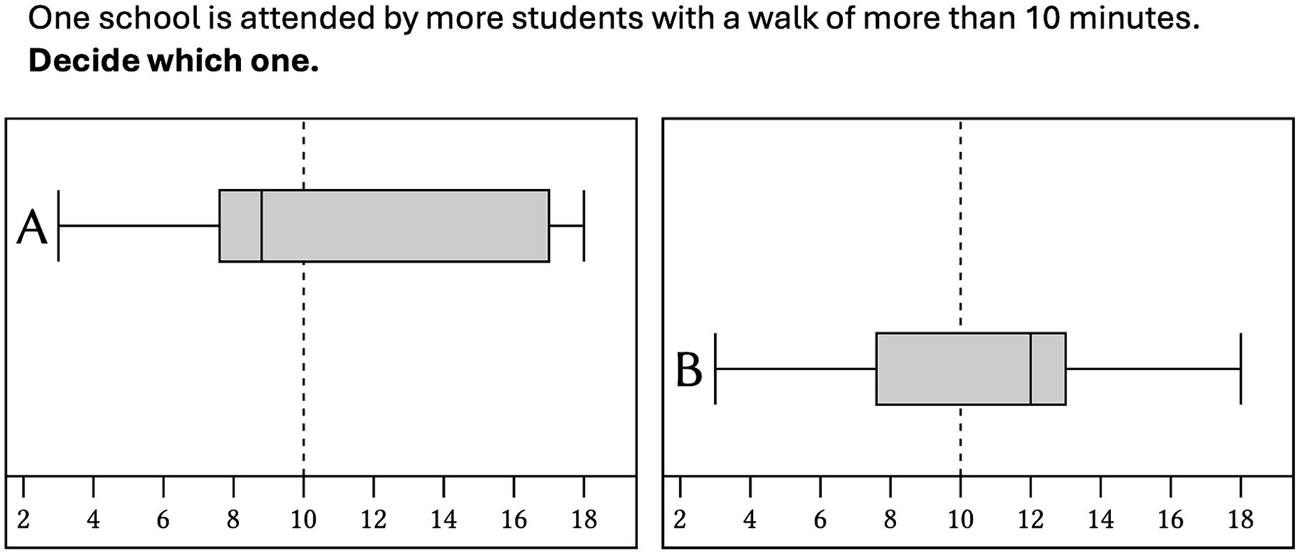
Figure 5. Example of an item in diagonal alignment (translated from German into English).
2.3 Procedure and technical equipment
The study was conducted in the university’s eye-tracking lab with a Tobii Pro Spectrum (600 Hz) between December 2022 and January 2023. The stimuli were displayed full screen on the monitor (Eizo FlexScan EV2451) with a screen diagonal of 23.8 inches, a resolution of 1920 × 1,080 and a refresh rate of 60 Hz. After participants were informed about the data collection by means of eye tracking, they gave their written consent to the anonymized data collection, storage, analysis, and academic use (including scientific publications). After setting up (70 cm distance from screen, free head moving) and performing a 5-point-calibration with validation (accuracy: M = 0,47°, SD = 0,15°, precision (SD): M = 0,23°, SD = 0,18°, precision (RMS): M = 0,16°, SD = 0,09°,) the participants were first presented with a single box plot for 10,000 ms with the instruction that the subsequent items were about this statistical representation. On two following slides, the task was presented (for detailed wording see Figure 3, in German translation) with the information that the task was the same in all following items. At this point, no example item with box plots was shown. Participants were informed that they would only see each of the following items for 10,000 ms seconds and were asked to give an answer within this time. In previous studies, 5,000 ms was chosen (Lem et al., 2013) as time restriction with the aim of inducing heuristic solution processes. Since this was not our goal, but at the same time we wanted to prevent learning during the assessment, we also used a time restriction but doubled the time. The 24 items were presented in a semi-random order: Each of the six item categories was only repeated after an item from all other categories had been shown. This order was the same for all participants. The participants could see each item for a maximum of 10,000 ms and gave the answer (school A or school B) by acclamation during this period. If the participants gave the answer before the 10,000 ms had elapsed, the next item was shown straight afterwards.
2.4 Data analysis
For each participant, two data sets were used for the data analysis: on the one hand, based on the answers given by each participant for each of the 24 items, information was available about whether this item was solved correctly or incorrectly. On the other hand, for each participant and each item, eye-tracking data that was recorded. The data was analyzed in a two-step process.
2.4.1 Grouping of participants based on solution patterns
Initially, regardless of the eye-tracking data, the solution patterns in the six different item categories were used to determine for each participant which schema was applied most likely in which of the two item types (median items and box items). In Table 1, the expected solution patterns are listed. If the individual solution rate that was achieved in an item category was greater than or equal to 0.5, this value was referred to as high, otherwise as low. Thus, each participant could either be assigned to a pattern or considered unclassifiable. For each participant and each schema (median schema, box schema and area schema), we then specified a dichotomous variable that takes the value 1 if the participant does apply the schema and the value 0 otherwise.
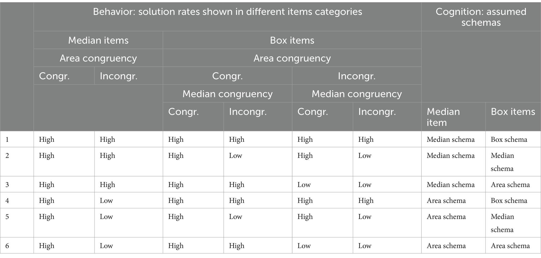
Table 1. Solution pattern and the corresponding schemas.
2.4.2 Defining areas of interest
In a second step, we defined disjoint AOIs for each item (Figure 6). For each of the two box plots, an AOI was defined for the first quartile (A1/B1), the median (A2/B2), the third quartile (A3/B3), and the dashed line highlighting the critical value (A4/B4). Although not required for the analysis, two theoretical AOIs were also defined for the minimum and maximum (gray fields, Figure 6) to determine the borders of the AOIs according to the following principle: The middle between two adjacent quartiles, respectively, between the line that indicates the critical value, and the adjacent quartiles represented the border of two adjacent AOIs. All AOIs were of the same height. Table 2 shows the average width of the AOIs, the height of all AOIs was the same (209 px/57 mm). We used the Tobii I - VT fixation filter to classify (threshold velocity of 30°/s) eye movement as part of a fixation or as a part of a saccade. For the fixation points, it was then determined in which AOI they were positioned. For each participant and for each schema, we summed up across all items how long (fixation duration), how often (number of fixations) the AOIs assumed to be relevant for the schema were fixated or how many transitions (transition count) were observed between these AOIs. The relevant AOIs were derived from the hypotheses: AOIs A2 and B2 were assumed to be relevant for the median schema, AOIs A1 and B1 for the box schema, and AOIs A3 and A4 or B3 and B4 for the area schema. For each participant, this resulted in three variables for each of the three schemas.
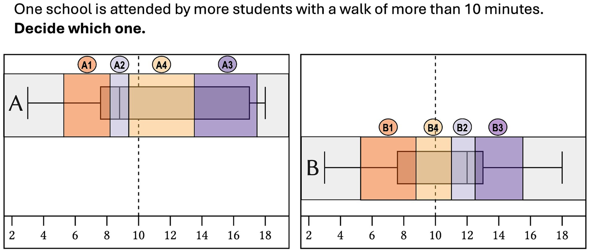
Figure 6. Example item (translated from German into English) with defined AOIs for the first quartile (A1/B1), the median (A2/B2), the third quartile (A3/B3) and the critical value (dashed line, A4/B4).
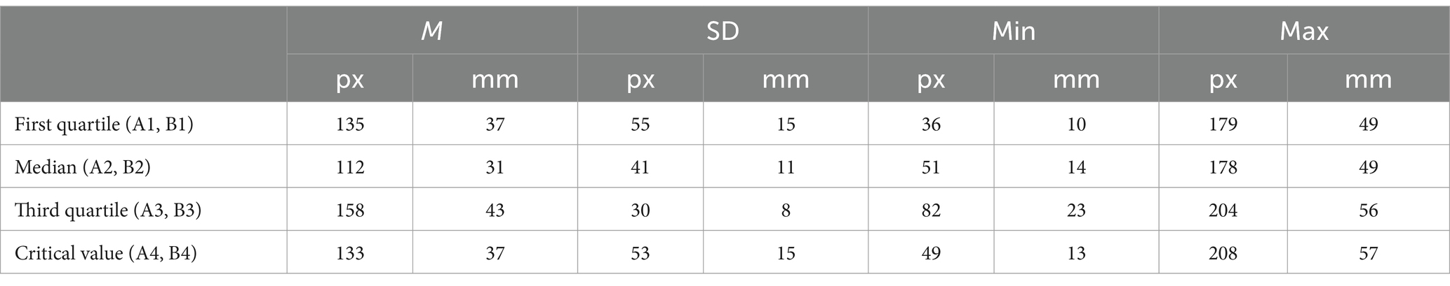
Table 2. Width of the AOIs.
2.4.3 Testing the hypotheses
In a third step, we tested the hypotheses by using the schemas determined based on the solution rates (see section 2.4.1) as independent variables and the variables determined from the eye-tracking data (2.4.2) as dependent variables to check the extent to which the assumed schema explained differences in eye movements. In the case of the hypotheses regarding the fixation duration, a linear model was used to check whether the participants fixed significantly longer on the relevant AOIs. In the case of the hypotheses regarding the number of fixations, a generalized linear model (poisson distributed) was used to check whether the participants showed a significantly higher number of fixations on the relevant AOIs. In the case of the hypotheses regarding the number of transitions, a generalized linear model (poisson distributed) was used to check whether the participants showed a significantly higher number of transitions between the relevant AOIs (Table 3).
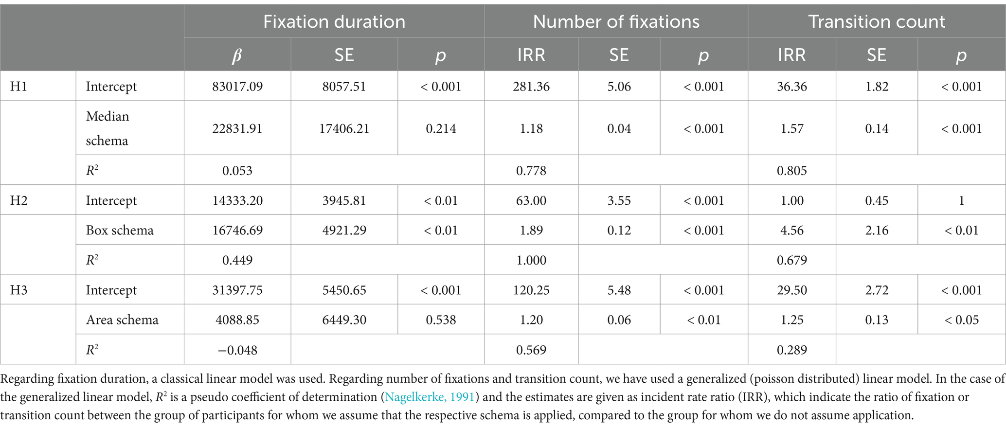
Table 3. Results of the (generalized) linear models.
3 Results
Overall, n = 13 participants could be assigned to a profile (Table 1) based on their solution patterns. For one participant, the solution pattern did not match any of the assumed profiles. A total of n = 3 participants showed high solution rates in both item types and thus could be assigned to the first profile. We therefore assumed that these participants used a median schema for median items and a box schema for box items. A total of n = 6 participants showed high solution rates in box items, in median items only if the item was area congruent and thus could be assigned to the fourth profile. We therefore assumed that these participants used a box schema for box items and an area schema for median items. A total of n = 4 participants showed high solution rates only in area-congruent items, but low solution rates in area-incongruent items (regardless of the item type) and thus could be assigned to the sixth profile. We therefore assumed that these participants used an area schema in both item types. For each of the three schemas, we report the results with regard to the fixation duration (hypothesis a), the number of fixations (hypothesis b) and the number of transitions (hypothesis c).
3.1 Median schema
We investigated whether participants who applied the median schema showed eye movement data that suggest a comparison of the medians. We assumed that this comparison is reflected on three levels: Firstly, we hypothesized (H1a) that the median schema becomes manifest in a longer fixation duration on the medians. Even if this effect was descriptively apparent, it was not statistically significant in our sample (β = 22831.91, 95%CI [−15092.97, 60756.79], p = 0.214). Secondly, we hypothesized (H1b) that the median schema becomes manifest in a higher number of fixations on the medians. We found this hypothesis supported by our sample (IRR = 1.18***, 95%CI [1.10, 1.27], p < 0.001). Thirdly, we hypothesized (H1c) that the median schema becomes manifest in more transitions between the two medians. We found this hypothesis supported by our sample (IRR = 1.57***, 95%CI [1.31, 1.87], p < 0.001).
3.2 Box schema
We investigated whether participants who correctly solved box items showed eye movement data that suggest a comparison of the first quartiles. We assumed that this comparison is reflected on three levels: Firstly, we hypothesized (H2a) that the box schema becomes manifest in a longer fixation duration on the first quartiles. We found this hypothesis supported by our sample (β = 16746.69**, 95%CI [6024.13, 27469.25], p < 0.01). Secondly, we hypothesized (H2b) that the box schema becomes manifest in a higher number of fixations on the first quartiles. We found this hypothesis supported by our sample (IRR = 1.89***, 95%CI [1.67, 2.15], p < 0.001). Thirdly, we hypothesized (H2c) that the box schema becomes manifest in more transitions between the two first quartiles. We found this hypothesis supported by our sample (IRR = 4.56***, 95%CI [1.98, 13.19], p < 0.01).
3.3 Area schema
We investigated whether participants who correctly solve only area congruent items show eye movement data that suggest a comparison of the area above the critical value. We assumed that this comparison is reflected on three levels: Firstly, we hypothesized (H3a) that the area schema becomes manifest in a longer fixation duration on the third quartiles and the critical value. Even if this effect was descriptively apparent, it was not significant in our sample (β = 4088.85, 95%CI [−9962.96, 18140.66], p = 0.538). Secondly, we hypothesized (H3b) that the area schema becomes manifest in a higher number of fixations on the third quartiles and the critical value. We found this hypothesis supported by our sample (IRR = 1.20**, 95%CI [1.08, 1.33], p < 0.01). Thirdly, we hypothesized (H3c) that the area schema becomes manifest in more transitions between the two first quartiles and the critical value. We found this hypothesis supported by our sample (IRR = 1.25***, 95%CI [1.02, 1.55], p < 0.05).
4 Discussion
Box plots are a widely used form of representation in descriptive statistics, but at the same time a challenging subject to learn. So far, research has identified different schemas based on systematically different solution rates in congruent and incongruent items that represent both appropriate and erroneous attempts to answer critical-value-comparison tasks. This study assumes that different box plot components are cognitively processed in the different schemas. With reference to the eye-mind assumption, we used eye tracking data to investigate whether these different cognitive processes are also reflected in different gaze pattern. In fact, for each schema, differences in the eye movement data could be identified that were in line with the assumptions: While the median schema includes a pairwise comparison of the medians and the box schema a pairwise comparison of the first quartiles as a characteristic feature, the area schema works primarily by focusing on the third quartiles, which represent the expansion of the area above the critical value. These results can not only provide validation of the schemas assumed based on the solution rates, but also indicate that critical-value-comparison tasks are solved by focusing on certain quartiles, where the quartiles that are particularly focused depend on the item configuration (median items / box items). Particularly noteworthy is the observation that although these differences in focus can be found across all schemas regarding the number of fixations and also regarding the number of transitions, the duration of fixations on the relevant AOIs is only significantly increased in the case of the median schema. One possible explanation could be that no text elements had to be encoded in the items used, but rather components of a diagram had to be perceived. It is possible that this form of perception requires less long but more frequent fixations.
The following rather methodological finding is related to this issue: There were participants who, based on their solution rates, were highly likely to consistently decide according to a particular schema. While the different schemas were visible in the eye-tracking data in the diagonal arrangement, it was not the case for the vertical arrangement. This raises some general questions about the interpretation of eye-tracking data for stimuli that do not require encoding of symbols. Obviously, participants were able to perceive relevant features of the items without explicitly focusing on them if they were within a certain radius of their actual fixation points (in the case of the vertical presentation).
The study is essentially subject to three limitations: First, the study investigated the extent to which eye movement data differed between groups that had previously been defined on the basis of solution rates in congruent and incongruent items. The differences in the eye movement data were then used on the one hand to validate these schemas, but primarily to describe the previously identified schemas in more detail. It is questionable whether the schemas can be identified solely based on eye movement data without the use of congruent and incongruent items. For this endeavor - and this is the second limitation - a substantially larger sample is required. It can also be expected that in a larger sample all theoretically assumed profiles (see table) would actually be assigned to one or more participants, which was not the case in the present study. Thirdly, a central assumption of our study is that the diagonal arrangement of the box plots is solely a matter of design and has no effect on the cognitive processes when comparing the box plots. Whether this is indeed the case should be confirmed by replicating the results using alternative designs. Overall, this study should therefore be considered as a feasibility test. However, the results provide promising indications that eye-tracking data can help to better understand cognitive processes when comparing statistical representations.
Data availability statement
The raw data supporting the conclusions of this article will be made available by the authors, without undue reservation.
Ethics statement
Ethical approval was not required for the studies involving humans because local legislation and authorities do not require this for the conducted kind of research and participants involved. The studies were conducted in accordance with the local legislation and institutional requirements. The participants provided their written informed consent to participate in this study.
Author contributions
MA: Conceptualization, Data curation, Formal analysis, Investigation, Methodology, Project administration, Resources, Validation, Visualization, Writing – original draft, Writing – review & editing. TL: Conceptualization, Funding acquisition, Methodology, Supervision, Validation, Writing – review & editing. KL: Conceptualization, Funding acquisition, Methodology, Supervision, Validation, Writing – review & editing. AS: Conceptualization, Data curation, Formal analysis, Methodology, Validation, Writing – review & editing. WD: Conceptualization, Methodology, Validation, Writing – review & editing. FR: Conceptualization, Data curation, Formal analysis, Funding acquisition, Investigation, Methodology, Project administration, Resources, Supervision, Validation, Visualization, Writing – review & editing.
Funding
The author(s) declare that financial support was received for the research, authorship, and/or publication of this article. This work was supported by the Baden-Wuerttemberg Ministry of Science, Research and Arts (grant number: 43–7742.35/24/1); and the University of Education Freiburg (grant number: 20204023). This publication was funded by the German Research Foundation (DFG) grant “Open Access Publication Funding/2023–2025/University of Education Freiburg (512888488)”.
Conflict of interest
The authors declare that the research was conducted in the absence of any commercial or financial relationships that could be construed as a potential conflict of interest.
Publisher’s note
All claims expressed in this article are solely those of the authors and do not necessarily represent those of their affiliated organizations, or those of the publisher, the editors and the reviewers. Any product that may be evaluated in this article, or claim that may be made by its manufacturer, is not guaranteed or endorsed by the publisher.
Footnotes
1. ^If the number of observations in the distribution is not divisible by four without remainder, this may result in subsets that are not exactly the same size. However, these differences are neglectable for a sufficiently large sample.
References
Abt, M., Loibl, K., Leuders, T., and Reinhold, F. (2022). Considering conceptual change as a source for errors when comparing data sets with boxplots. EARLI SIG3. Zwolle, The Netherlands.
Abt, M., Loibl, K., Leuders, T., Van Dooren, W., and Reinhold, F (2024). Understanding Student Errors in Comparing Data Sets with Boxplots.
Abt, M., Reinhold, F., and Van Dooren, W. (2023). Revealing cognitive processes when comparing box plots using eye-tracking data—a pilot study. Proceedings of the 46th conference of the International Group for the Psychology of mathematics education, 11–18.
Andrà, C., Arzarello, F., Ferrara, F., Holmqvist, K., Lindström, P., Robutti, O., et al., (2009). How students read mathematical representations: an eye tracking study. Proceedings of the33rd conference of the International Group for the Psychology of mathematics education, 49–56.
Bakker, A., Biehler, R., and Konold, C. (2005). “Should young students learn about box plots?” in Curricular Development in Statistics Education. eds. G. Burrill and M. Camden (Lund, Sweden: International Association for Statistical Education), 163–173. Available at: https://iase-web.org/documents/papers/rt2004/1_Frontmatter.pdf?1402524986
Behrens, J. T., Stock, W. A., and Sedgwick, C. (1990). Judgment errors in elementary box-plot displays. Comm. Stat. Sim. Comp. 19, 245–262. doi: 10.1080/03610919008812855
Ben-Zvi, D., Makar, K., and Garfield, J. B. (Eds.) (2018). International handbook of research in statistics education. Cham, Switzerland: Springer International Publishing.
Biehler, R. (1997). “Students’ difficulties in practicing computer-supported data analysis: some hypothetical generalizations from results of two exploratory studies” in Research on the Role of Technology in Teaching and Learning Statistics. eds. J. Garfield and G. Burrill (Granada, Spain: International Statistical Institute), 176–197.
Boels, L., Bakker, A., and Drijvers, P. (2019). Eye-tracking secondary school students’ strategies when interpreting statistical graphs. Proceedings of the 43rd Conference of the International Group for the Psychology of mathematics education, 113–120.
Chi, M., Glaser, R., and Rees, E. (1982). “Expertise in problem solving” in Advances in the psychology of human intelligence. ed. R. Sternberg, vol. 1 (Hillsdale, NJ: Lawrence Erlbaum Associates), 7–75.
Cobb, G. W., and Moore, D. S. (1997). Mathematics, statistics, and teaching. Am. Math. Mon. 104, 801–823. doi: 10.1080/00029890.1997.11990723
delMas, R. C. (2004). “A comparison of mathematical and statistical reasoning” in The challenge of developing statistical literacy, reasoning and thinking. eds. D. Ben-Zvi and J. B. Garfield (Netherlands: Springer), 79–95.
Edwards, T. G., Özgün-Koca, A., and Barr, J. (2017). Interpretations of boxplots: helping middle school students to think outside the box. J. Stat. Educ. 25, 21–28. doi: 10.1080/10691898.2017.1288556
Finger, F. W., and Spelt, D. K. (1947). The illustration of the horizontal-vertical illusion. J. Exp. Psychol. 37, 243–250. doi: 10.1037/h0055605
Garfield, J. B., and Ben-Zvi, D. (2008). Developing students’ statistical reasoning: Connecting research and teaching practice. New York, USA: Springer.
Holmqvist, K., Nyström, M., Andersson, R., Dewhurst, R., Jarodzka, H., de Weijer, V., et al. (2011). Eye tracking: A comprehensive guide to methods and measures. Oxford (GB) and New York (USA): Oxford University Press.
Just, M. A., and Carpenter, P. A. (1980). A theory of reading: from eye fixations to comprehension. Psychol. Rev. 87, 329–354. doi: 10.1037/0033-295X.87.4.329
Kader, G., and Perry, M. (1996). To boxplot or not to boxplot? Teach. Stat. 18, 39–41. doi: 10.1111/j.1467-9639.1996.tb00279.x
Kramer, R. S. S., Telfer, C. G. R., and Towler, A. (2017). Visual comparison of two data sets: do people use the means and the variability? J. Numer. Cog. 3, 97–111. doi: 10.5964/jnc.v3i1.100
Krzywinski, M., and Altman, N. (2014). Visualizing samples with box plots. Nat. Methods 11, 119–120. doi: 10.1038/nmeth.2813
Lai, M.-L., Tsai, M.-J., Yang, F.-Y., Hsu, C.-Y., Liu, T.-C., Lee, S. W.-Y., et al. (2013). A review of using eye-tracking technology in exploring learning from 2000 to 2012. Educ. Res. Rev. 10, 90–115. doi: 10.1016/j.edurev.2013.10.001
Lem, S., Onghena, P., Verschaffel, L., and Van Dooren, W. (2013). The heuristic interpretation of box plots. Learn. Instr. 26, 22–35. doi: 10.1016/j.learninstruc.2013.01.001
Lilienthal, A., and Schindler, M. (2019). “Current trends in the use of eye tracking in mathematics education research: a PME survey” in Proceedings of 43rd annual meeting of the International Group for the Psychology of mathematics education, vol. 4, 62.
Masnick, A. M., and Morris, B. J. (2008). Investigating the development of data evaluation: the role of data characteristics. Child Dev. 79, 1032–1048. doi: 10.1111/j.1467-8624.2008.01174.x
Massart, D. L., Smeyers-Verbeke, J., Capron, X., and Schlesier, K. (2005). Visual presentation of data by means of box plots.
Nagelkerke, N. J. D. (1991). A note on a general definition of the coefficient of determination. Biometrika 78, 691–692. doi: 10.1093/biomet/78.3.691
National Council of Teachers of Mathematics. (2000). Principles and standards for school mathematics. National Council of Teachers of Mathematics.
Obrecht, N. A., Chapman, G. B., and Gelman, R. (2007). Intuitivet tests: lay use of statistical information. Psychon. Bull. Rev. 14, 1147–1152. doi: 10.3758/BF03193104
Ott, N., Brünken, R., Vogel, M., and Malone, S. (2018). Multiple symbolic representations: the combination of formula and text supports problem solving in the mathematical field of propositional logic. Learn. Instr. 58, 88–105. doi: 10.1016/j.learninstruc.2018.04.010
Posner, G. J., Strike, K. A., Hewson, P. W., and Gertzog, W. A. (1982). Accommodation of a scientific conception: toward a theory of conceptual change. Sci. Educ. 66, 211–227. doi: 10.1002/sce.3730660207
Reading, C., and Shaughnessy, J. M. (2004). “Reasoning about variation” in The challenge of developing statistical literacy, reasoning and thinking. eds. D. Ben-Zvi and J. B. Garfield (Netherlands: Springer), 201–226.
Rumelhart, D. E., McClelland, J. L., and Hinton, G. E. (1986). “Schemata and sequential thought processes in PDP models” in Parallel Distributed Processing: Explorations in the Microstructure of Cognition: Psychological and Biological Models (Cambridge: The MIT Press).
Schindler, M., and Lilienthal, A. J. (2019). Domain-specific interpretation of eye tracking data: towards a refined use of the eye-mind hypothesis for the field of geometry. Educ. Stud. Math. 101, 123–139. doi: 10.1007/s10649-019-9878-z
Schreiter, S., and Vogel, M. (2023). Eye-tracking measures as indicators for a local vs. global view of data. Front. Educ. 7:1058150. doi: 10.3389/feduc.2022.1058150
Shaughnessy, J. M. (1997). Missed opportunities in research on the teaching and learning of data and chance. Hamilton: MERGA, 1997.
Streit, M., and Gehlenborg, N. (2014). Bar charts and box plots. Nat. Methods 11:117. doi: 10.1038/nmeth.2807
Strohmaier, A. R., MacKay, K. J., Obersteiner, A., and Reiss, K. M. (2020). Eye-tracking methodology in mathematics education research: a systematic literature review. Educ. Stud. Math. 104, 147–200. doi: 10.1007/s10649-020-09948-1
Strohmaier, A. R., Reinhold, F., Hofer, S., Berkowitz, M., Vogel-Heuser, B., and Reiss, K. (2022). Different complex word problems require different combinations of cognitive skills. Educ. Stud. Math. 109, 89–114. doi: 10.1007/s10649-021-10079-4
Vosniadou, S., and Verschaffel, L. (2004). Extending the conceptual change approach to mathematics learning and teaching. Learn. Instr. 14, 445–451. doi: 10.1016/j.learninstruc.2004.06.014
Watson, J. M. (2006). Statistical literacy at school: Growth and goals. Mahwah, NJ: L. Erlbaum Associates.
Keywords: box plots, misinterpretation, systematic error, conceptual change, schema-based reasoning, statistical literacy, eye-tracking
Citation: Abt M, Leuders T, Loibl K, Strohmaier AR, Van Dooren W and Reinhold F (2024) How can eye-tracking data be used to understand cognitive processes when comparing data sets with box plots? Front. Educ. 9:1425663. doi: 10.3389/feduc.2024.1425663
Edited by:
Joaquin Marc Veith, University of Hildesheim, GermanyReviewed by:
Julia Sirock, Heidelberg University of Education, GermanyMehmet Fatih Öçal, Ağrı İbrahim Çeçen University, Türkiye
Copyright © 2024 Abt, Leuders, Loibl, Strohmaier, Van Dooren and Reinhold. This is an open-access article distributed under the terms of the Creative Commons Attribution License (CC BY). The use, distribution or reproduction in other forums is permitted, provided the original author(s) and the copyright owner(s) are credited and that the original publication in this journal is cited, in accordance with accepted academic practice. No use, distribution or reproduction is permitted which does not comply with these terms.
*Correspondence: Martin Abt, bWFydGluLmFidEBwaC1mcmVpYnVyZy5kZQ==