Meta-critical thinking, paradox, and probabilities

There is as much lack of clarity concerning what “critical thinking” involves, even among those charged with teaching it, as there is consensus that we need more emphasis on it in both academia and society. There is an apparent need to think critically about critical thinking, an exercise that might be called meta-critical thinking. It involves emphasizing a practice in terms of which “critical thinking” is helpfully carried out and clarifying one or more of the concepts in terms of which “critical thinking” is usually defined. The practice is distinction making and the concept that of evidence. Science advances by constructing models that explain real-world processes. Once multiple potential models have been distinguished, there remains the task of identifying which models match the real-world process better than others. Since statistical inference has in large part to do with showing how data provide support, i.e., furnish evidence, that the model/hypothesis is more or less likely while still uncertain, we turn to it to help make the concept more precise and thereby useful. In fact, two of the leading methodological paradigms—Bayesian and likelihood—can be taken to provide answers to the questions of the extent to which as well as how data provide evidence for conclusions. Examining these answers in some detail is a highly promising way to make progress. We do so by way of the analysis of three well-known statistical paradoxes—the Lottery, the Old Evidence, and Humphreys’—and the identification of distinctions on the basis of which their plausible resolutions depend. These distinctions, among others between belief and evidence and different concepts of probability, in turn have more general applications. They are applied here to two highly contested public policy issues—the efficacy of COVID vaccinations and the fossil fuel cause of climate change. Our aim is to provide some tools, they might be called “healthy habits of mind,” with which to assess statistical arguments, in particular with respect to the nature and extent of the evidence they furnish, and to illustrate their use in well-defined ways.

1 Introduction

“I do not feel obliged to believe that the same God who has endowed us with sense, reason, and intellect has intended us to forgo their use” Galileo—Letter to the Grand Duchess Christina.

It has been said:

While there is general agreement that critical thinking is important, there is less consensus, and often lack of clarity, about what exactly constitutes critical thinking. For example, in a California study, only 19 percent of faculty could give a clear explanation of critical thinking even though the vast majority (89 percent) indicated that they emphasize it (Stassen et al., 2011).

The problem is 2-fold. On the one hand, the conventional treatment of critical thinking is general not specific, often suggests a perspective or frame of mind, and does not provide a set of skills, still less a handy set of tools with which to exercise them or criteria for their application.¹ On the other hand, it is not usually made clear what the aim or outcome of critical thinking is (Schmaltz et al., 2017).

1.1 Why is the ability to think critically to be prized?

To provide still another definition of “critical thinking” at this point would be of little use. We are better advised to focus on the concepts in terms of which it is most often characterized, an exercise in what might be called meta-critical thinking. This sort of second-order reflection applies equally to the conduct of one’s own research, the evaluation of scientific results published by others, and the settling of public policy and other issues of general concern in which such studies often play a large role. As the previous sentence indicates, scientific inference occurs at multiple levels. Scientists are individuals and learn on a personal level. Science, on the other hand, is a collective activity. Learning in Science, writ large, is a massively collective activity involving communication (much of which is indirect) among every scientist living, every scientist who has ever lived, and everything they have ever written. Different levels may require different inferential tools (for a discussion of public versus private epistemology see Taper and Ponciano, 2016).

Slogans like “make only evidence-based claims” are everywhere in the critical thinking literature and to the best of our knowledge are left largely undefined and vague.² Since statistical inference has to do in large part with showing how data provide support, i.e., evidence, for more or less likely conclusions, we are well advised to turn to it to make the concept more precise and thereby useful. As will be shown, the leading inferential methodologies in statistics³ can be taken to provide answers to the questions: to what extent and how data provide evidence to support conclusions? The fact that statistical inferences are commonly made in all of the sciences underlines the importance of examining these methodologies in some detail.

Too often the case is made for a particular claim that has far spreading public policy implications on the basis of an alleged “consensus of experts,” without any attempt to indicate the reasoning on the basis of which these claims are made.⁴ It is the ability of citizens to appreciate in general terms how central scientific claims are tested and come to be accepted that is a fundamental feature of democratic societies and should be a cornerstone of all STEM education.⁵ This is all the more important at a time when the general acceptance or rejection of these conclusions has increasingly been politicized.⁶ It should not be surprising as a result that there is a growing lack of confidence in science on the part of the general public and a corresponding distrust of “experts” and “elites,” a key ingredient in populist politics.⁷

For example, although more than 99.9% of published studies agree that climate change is due more to human activities than natural conditions (Lynas et al., 2021),⁸ recent polling indicates that no more than 64% of the general population agrees (Saad et al., 2021).⁹ Similarly, although the Pfizer-BioTech and Moderna vaccines were shown to be more than 95% effective against the original coronavirus strain in Phase 3 clinical trials and continued to be so at the same rate against SARS-CoV-2 variants through 2021, only 55% of Americans polled agree that vaccination is “extremely or very effective” at limiting coronavirus spread (Kennedy et al., 2022). Of course, both climate change and the coronavirus have become deeply partisan political issues, with elected officials offering and occasionally institutionalizing their own uninformed takes. We will return to these examples of human-caused climate change or the effectiveness of COVID vaccines in more detail later. Not surprisingly, a recent Gallup Poll reports a long-term decrease of confidence in the scientific community from 70% in 1975 to 64% in 2021 (Boyle, 2022). The reasons for this decline are undoubtedly manifold, but it is clear that in part the decline is due to perceptions by the public of bias on the part of scientists. Many Pew poll responders indicated they did not believe that scientists had the public’s best interest at heart (Kennedy et al., 2022). Other Pew research shows that 35% of the American population think the scientific method can be used to produce “any result a researcher wants” (Funk, 2020). Our aim is to provide and illustrate some general but very useful ways of assessing the statistical arguments on which the “consensus of experts” (genuine as well as Self-proclaimed) among other sources of statistical claims is assumed to rest, in particular with respect to the nature and extent of the evidence they should be expected to furnish. The end product is a list of “healthy habits of mind” to use whenever confronted with such arguments and the main question asked concerns their evidential force.

1.2 The purposes of paradoxes

The task is clear: to think critically about statistical inference, identify distinctions that both aid in doing so and have more general application, and in the process develop helpful “habits of mind” to use when confronted with statistical claims and the arguments on which they are based. How to proceed? One traditionally productive way to do so is by way of reflecting on paradoxes, conclusions that seem absurd and are on occasion self-contradictory, but are entailed by premises that are plausible if not also obvious. Short of being willing to grant on reflection that the conclusion is not so absurd after all or finding Zen comfort in perplexity, there are two ways as a matter of logic to unravel paradoxes, either reject one of the premises or show that the paradoxical conclusion does not follow from them. To these two, we add a useful third; disarm the paradox by showing that it rests on an equivocation:

List 1: Methods of unraveling paradoxes

I Show that at least one of the premises required for its derivation is false, in which case the derivation is not sound, i.e., though the argument is valid the conclusion is not necessarily true.

II Show that an argument of the same form can have true premises and a false conclusion, in which case the argument is not valid.

III Disarm the paradox by showing that it rests on an equivocation, that is, amalgamates two concepts that should be kept distinct or demonstrates that two traditionally distinct concepts should be assimilated so as to distinguish both of them from a third.

The third way of unraveling paradoxes, by drawing a new distinction (sometimes after undermining an old), has often proved the most fruitful. That is, the critical and creative thinking involved in disarming paradoxes has historically cleared a path to progress (see Box 1 for two classic examples).

BOX 1. Two transformative scientific paradoxes

For the benefit of those readers unfamiliar with the analysis of paradoxes, we look briefly at two notable mathematical and physical examples, draw some lessons from them as concerns the distinctions they draw, and illustrate the benefits of drawing these distinctions.

Galileo’s paradox of infinity

The first of our examples has to do with a basic mathematical concept, infinity, the second with a basic physical concept, motion. Both were made famous by Galileo.

Galileo was not the first to demonstrate the paradoxical character of infinite sets. Among others, the philosopher Duns Scotus noted in 1302 that although intuitively there are half as many even numbers as there are whole numbers, on reflection there are an infinite number of each, i.e., there are as many even numbers as whole numbers. Nevertheless, the paradox has come to be associated with Galileo. In his final scientific work, the Dialogues Concerning Two New Sciences Galileo’s spokesperson, Salviati concludes:

So far as I can see we can only infer that the totality of all numbers is infinite, that the number of squares is infinite, and that the number of their roots is infinite; neither is the number of squares less than the totality of all the numbers, nor the latter greater than the former; and finally the attributes ‘equal,’ ‘greater,’ and ‘less,’ are not applicable to infinite but only to finite quantities (Galileo Galilei, 1638).

Salviati goes on to draw the corollary that “longer” lines do not contain more points than “shorter,” but that each line contains an infinite number. There the matter stood—that a set can have multiple proper subsets, all of the same size as the parent set, so long as both sets and subsets are infinite and that infinite sets cannot be compared to one another with respect to size—until Georg Cantor in 1874 was able to provide a proof (Cantor, 1874) that at least some (“uncountable”) sets, e.g., the set of real numbers, cannot be put into one-to-one correspondence with any of their proper (“countable”) subsets, e.g., the set of rationals. Thus, it is therefore possible, indeed necessary, to say of at least some infinite sets that they are equal to, greater than, or less than others. In the process, he drew a finer distinction between different senses of “equal,” “greater,” and “less,” and disarmed the paradox that some sets of numbers are apparently smaller than others and at the same time equal in size to them by reformulating and embracing the first of its premises.

Galileo’s paradox of motion

A second Galilean paradox has to do with the relativity of motion. It exemplifies a conflict between what we observe and what a theory postulates. The theory in question is Copernicus’ revolutionary two-part claim that the earth both revolves around the sun and rotates on its own axis. Galileo wrote Dialogues Concerning Two New Sciences of 1632 to defend this theory (and the Euclidean geometry used to expound it, hence his disarming the criticism that longer and shorter lines could not, as against that geometry, contain equal and infinite numbers of points) against the criticisms commonly made of it, the majority of which had to do with the fact that the claim flew in the face of observation.

If the earth revolved around the sun, then the 24-h passage from day to night and back again that we observe could only be explained by the earth’s rotating on its axis at a notable speed, in which case we would sense the motion internally and observe untethered objects moving west. But when lying in bed at night we do not feel like we are moving and during the day we do not see balls tossed in the air invariably land to the west of us. These simple observations would seem to entail that the Copernican hypothesis is false, the earth does not rotate on its axis and still less around the sun.

To counter this argument, Galileo’s spokesperson, Salviati, develops a thought experiment.

Shut yourself up with some friend in the main cabin below decks on some large ship, and have with you there some flies, butterflies, and other small flying animals. Have a large bowl of water with some fish in it; hang up a bottle that empties drop by drop into a wide vessel beneath it. With the ship standing still, observe carefully how the little animals fly with equal speed to all sides of the cabin. The fish swim indifferently in all directions; the drops fall into the vessel beneath; and, in throwing something to your friend, you need to throw it no more strongly in one direction than another, the distances being equal; jumping with your feet together, you pass equal spaces in every direction. When you have observed all these things carefully (though doubtless when the ship is standing still everything must happen in this way), have the ship proceed with any speed you like, so long as the motion is uniform and not fluctuating this way and that. You will discover not the least change in all the effects named, or could you tell from any of them whether the ship was moving or standing still (Galileo Galilei, 1632, p. 186).

The paradox—the apparent contradiction between theory and observation, to wit, between motion and rest, is explained away by showing that there is no principled way to distinguish between them so long as the motion is uniform.

2 The discipline of distinction-making

The importance of distinctions underlined, it is worthwhile to pause for a moment and reflect briefly on four criteria that in our view should be satisfied before making them if distinctions are to play a useful role. It will shortly be made clear how these criteria apply and why they are useful.

List 2: Useful distinction criteria

I Should make a difference, i.e., no genuine difference, no distinction.¹⁰

II Should be clear: There must be some hallmark or feature on the basis of which the distinction can be made.

III Should be insightful: Adequate distinctions should serve to unify or explain facts and ideas in a new and interesting way.

IV Should be applicable to more topics of concern than the paradox at hand, i.e., must not be ad hoc.

2.1 Paradoxically useful distinctions

Now to the nub of the narrative. A failure to recognize a few critical distinctions is at the heart of a great deal of misunderstanding in statistics. This is to say that terms with very different meanings are often used interchangeably, that is the terms are equivocated. The result, as we will go on to demonstrate, is the source of misunderstandings and mistakes. We outline here five particularly important distinctions, which we will use to resolve three statistical paradoxes. Becoming aware of these distinctions may not make statistics easy, but it will make you aware of when you are entering a minefield and should keep you safer when the time comes.

The rest of this article depends heavily on the distinction between probability and likelihood, and the related distinction between conditioning on a random variable and conditioning on a fixed value. We understand that readers will come to the article with varying degrees of statistical background. To mitigate this discrepancy, we have provided two explanations—one on probability, a second on likelihood—in Boxes 2 and 3. Since they serve the role of extended footnotes, the reader can bypass them and nonetheless follow the main line of argument.

BOX 2. A précis of probability

Probability is a word whose meaning seems clear until you start to think about it. Then things get very fuzzy. If you look that term up, you will often find a definition like this one copied from an educational website: “Probability is simply how likely something is to happen”. This seems helpful but is not. If you look the word up in an English dictionary you will see that probable is defined as likely; and likely is defined as probable. In statistics, the terms probability and likelihood while intimately related, like the face and backside of a coin, mean very different things.

Terminology

Experiment

An experiment is a repeatable procedure with clearly defined possible outcomes. If there are more than one possible outcomes, and which will occur is uncertain, then the procedure is a random experiment. Flipping a coin is an experiment. The procedure is repeatable and has the uncertain defined outcomes of heads (H) or tails (T). A single iteration of the procedure is often called a trial.

Sample space

The sample space of an experiment is the set of all possible outcomes of the experiment. Outcomes should be thought of as primitive in that only one outcome can occur at a time. The sample space for the coin flip experiment is the set {H, T}. The sample space is often denoted by the symbol S.

Probability

Somethings/objects/sets/outcomes can be said to have a probability if for each object, a weight can be assigned following three rules: (1) all weights are greater than 0. (2) The weight of the union of two outcomes is equal to the sum of the weights of each outcome. And (3) The sum of the weights for all outcomes equals 1. Weights defined this way are called probabilities (Kolmogorov, 1956). If the outcomes are not categorical but are instead continuous an outcome point technically has a probability density, which only becomes a probability, in strict notation, when integrated over an interval or region and the sums are replaced by integrals. Note that more than just the mathematical definition of probabilities will be needed for these weights to be scientifically useful. In coin flip sample-space, we might say either based on a deductive assumption or based on experience with many repetitions that each of the outcomes {H} and {T} has a probability of ½.

Event

An event is a defined outcome or set of outcomes or set of other events The set of all possible events is generally designated as Ω. Technical choices in how Ω is constructed lead to different kinds of probability. The probability of an event is the sum of the probabilities of the outcomes that comprise it. If the experiment is to flip a coin twice, your sample space is the set {(H,H), (H,T), (T,H),(T,T)}. Each of these outcomes have probabilities of ¼. If an event, E₁, is defined as a two-tuple having one head and one tail, then the event is the set {(H,T), (T,H)}. The probability of this event is ¼ + ¼ = ½. Note that an outcome might be a member of more than one event. For instance, if E₂ is defined as all tuples containing at least 1 tail then E₂ = {(H,T),(T,H),(T,T)}, and the outcome (T,H) is a member of both E₁ and E₂. Because of this overlap, the probability of E₃ = (E₁,E₂) is not the sum of the probability of E₁ and the probability of E₂, but needs to be adjusted so the probability of any outcomes on which they overlap is not counted twice.

Random draw

A random draw selects one outcome from the sample-space. Which outcome will be selected is not determined or known before the draw. In an infinite series of draws, each possible outcome will occur in proportion to its probability. This property is a consequence of a mathematical theorem known as the Law of Large Numbers and forms one of the ways of defining probability for scientific applications.

Random variable

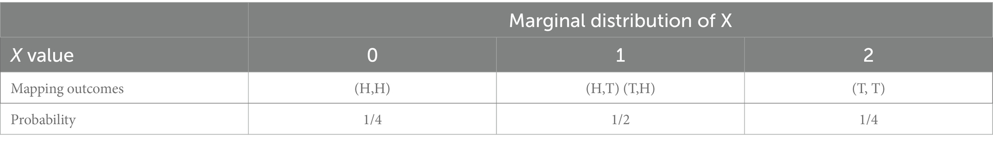
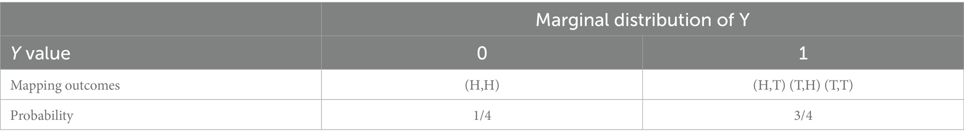
A random variable is a function that maps the collection of all events of an experiment to a set on numerical values, which can be integers, real, imaginary, or complex numbers. The function can be applied to any of the elements of the sample-space deterministically. The function only becomes a random variable if it is applied to a random draw from the sample-space. Random variables are generally denoted by italic uppercase roman letters such as X or Y. A random variable applied to a random draw returns a realization of the random variable, often called observation. Realizations/observations are generally designated an italic lower-case letter corresponding to the random variable such as x or y. The notation for probability is usually Pr(X = x). This is read as the probability that the random variable X takes on the value x. Often for the notation is shortened to Pr(x). This is compact but suppresses the information that probabilities are functions of random variables. It is critical to recognize that realizations/observations are no longer random. Two example random variables definitions are: (1) let X be a random variable that maps outcomes of the double coin flip experiment to the count of the number of its tails. X can have the values 0, 1, or 2. (1) Let Y be the random variable that maps outcomes to the presence or absence of tails. Y has the values 0 or 1.

Marginal probability

The marginal probability for a given value of a random variable is the probability that a random draw from the experiment will be mapped by the random variable to that particular value. Following rule 2 from the definition of probability, the marginal probability will be the sum of the probabilities of all the outcomes that map to the value.

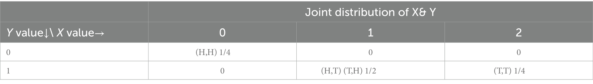
Joint probability

The joint probability distribution of two (or more) random variables is the set of all possible combinations of the values of the random variables with probabilities that are given by the sum of all outcomes that map to the particular combinations. Because the joint probability is a probability, the sum of the probabilities of all possible combinations must be 1.

Probability conditioned on a random variable

Because different events can share outcomes, knowing the value of one random variable can strongly influence your assessment of the probabilities for other random variables. This new probability is written verbosely as Pr(X = x|Y = y) and read as the probability that the unknown value of variable X will be x given that Y has been observed to have a value of y.

Continuing the coin tossing example, if y is observed to be 0 then the only possible outcome is (H,H) and the realized value of X must also be 0. Therefore Pr(X = 0|Y = 0) = 1, Pr(X = 1|Y = 0) = 0, and Pr(X = 2|Y = 0) = 0. If y is observed to be 1, the outcomes that can map to 1 are (H,T), (T,H), and (T,T). The conditional distribution of X is very different. The universe of possible outcomes is smaller than the sample-space but the conditional probabilities still need to sum to 1. The conditional probabilities can be calculated by dividing the joint probabilies of X and Y, Pr(X = x, Y = y), by the marginal probabilities of Y, Pr(Y = y). Note that Pr(X|Y) is generally not equal to Pr(Y|X). In our double coin flip experiment, Pr(X = 2|Y = 1) =2/3, but Pr(Y = 1|X = 2) = 1.

Bayes’ rule

An interesting and useful fact about conditional probabilities is that they are invertable: If you have two random variables, say X and Y, if you know both marginal probabilities and one conditional probability then you can calculate the other conditional probability. That is:

$a)\mathrm{Pr}\left(X|Y\right)=\frac{\mathrm{Pr}\left(Y|X\right)\mathrm{Pr}\left(X\right)}{\mathrm{Pr}\left(Y\right)},\text{and}\mathrm{b})\mathrm{Pr}\left(Y|X\right)=\frac{\mathrm{Pr}\left(X|Y\right)\mathrm{Pr}\left(Y\right)}{\mathrm{Pr}\left(X\right)}$

These formulae seem abstract, but can be understood in terms of the simple geometry of the portioning of the sample space by random events/variables.

Figure B2.1

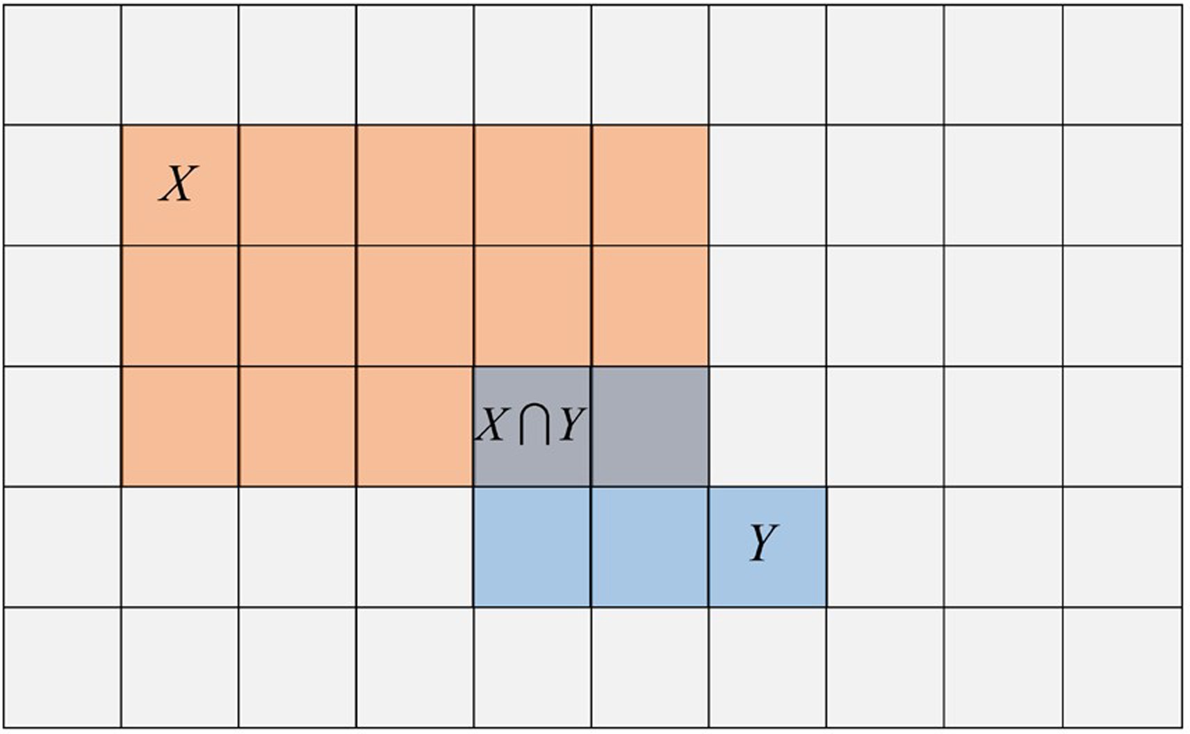
Figure B2.1. A geometric interpretation of Bayes’ rule. The probability space is the set of all squares, primitive outcomes, which here all have equal probabilities. The event X is the 15 squares with red tint. The event Y is the five squares with blue tint. The intersection of X and Y,$X\cap Y$, are the two primitive observations that are in both X and Y. Having both red and blue tints these observations appear as purple.

In the entire sample space there are 60 squares each having a probability of occurring of 1/60. Two of those observations are both X and Y so Pr(X&Y) = 2/60. If you told that your event is an X, then the universe of possible observations has been reduced from 60 to 15. In this smaller sample space, the probability of your event also being Y is now two chances out of 15 or 0.133.

What makes Bayes’ rule seem confusing when represented algebraically as opposed to geometrically is that the numerators of equations (a) and (b) above are written differently but represent the same value, the joint probability of X and Y:

$\mathrm{Pr}\left(Y|X\right)\mathrm{Pr}\left(X\right)=\mathrm{Pr}\left(X|Y\right)\mathrm{Pr}\left(Y\right)=\mathrm{Pr}\left(X\&Y\right).$

The correlation between random variables is defined as:

$\frac{\rho \left(X,Y\right)}{\sqrt{Var\left(X\right)Var\left(Y\right)}}=\mathrm{cov}\left(X,Y\right)$

Plugging in basic formulae for the variances and co-variances of random variables (following Conover, 1980, pages 38 and 39), an inter-class correlation coefficient for categorical events over a sample space can be written as:

$\rho \left(X,Y\right)=\frac{\mathrm{Pr}\left(X\&Y\right)-\mathrm{Pr}\left(X\right)\mathrm{Pr}\left(Y\right)}{\sqrt{\mathrm{Pr}\left(X\right)\left(1-\mathrm{Pr}\left(X\right)\right)\mathrm{Pr}\left(Y\right)\left(1-\mathrm{Pr}\left(Y\right)\right)}}$

Remembering that Pr(X & Y) = Pr(Y|X) Pr(X) and with some algebraic manipulation, Bayes’ rule can be rewritten as:

$\mathrm{Pr}\left(X|Y\right)=\left(\left(\rho \left(X,Y\right)g{\stackrel{-}{V}}_{XY}\right)+\mathrm{Pr}\left(X\right)\mathrm{Pr}\left(Y\right)\right)\frac{\mathrm{Pr}\left(X\right)}{\mathrm{Pr}\left(Y\right)}$

Where $g{\stackrel{-}{V}}_{XY}$ is the geometric mean of the variances of X and Y, i.e., the denominator of a correlation.

In Figure B2.1, the primitive outcomes are represented as squares, but this is just for convenience so that the probabilities represented by events can be calculated by counting. If the underlying sample space is continuous, the event polygons simply become closed curves with the probability of an event (or the random variable mapping to an event) represented by the enclosed area. Events are always categorical. This follows from the set definition of an event. Primitive outcomes are either in the event or they are not. Consequently, the recasting of Bayes’ rule in terms of correlation holds regardless if the underlying sample space is discrete or continuous.

BOX 3. A précis of likelihood

Parametric statistical models

Models describe features of the world. A statistical or stochastic model includes randomness among the features that it describes. A parameter is a numeric value or vector of values that controls the behavior of a model. Perhaps the most familiar statistical model in the world is the normal, or Gaussian, probability distributrion model:

$N\left(x;\mu ;\sigma \right)=\frac{1}{\sigma \sqrt{2\pi }}\exp \left(\frac{{\left(x-\mu \right)}^2}{2{\sigma }^2}\right),\begin{array}{c}-\infty <x<\infty \\ -\infty <\mu <\infty \\ 0<\sigma <\infty \end{array}$

Where x represents potential data. $N\left(x;\mu ;\sigma \right)$ is a function of x that returns ${\mathrm{Pr}}_d\left(X=x\right)$ given the specific values of $\mu$ and $\sigma$. The parameter $\mu$ is the mean or central value of the distribution, while $\sigma$ is the standard deviation or spread of the distribution. We saw earlier that ${\mathrm{Pr}}_d\left(x\right)$ is a shorthand notation for ${\mathrm{Pr}}_d\left(X=x\right)$. Now we see that this itself is a shorthand for ${\mathrm{Pr}}_d\left(X=x;\theta \right)$, which itself is a shorthand for ${\mathrm{Pr}}_d\left(X=x;M=m_i;\Theta ={\theta }_i\right)$, where m_i is a specific model and ${\theta }_i$ is model i’s parameter or parameter vector.

Conditioning on a fixed value

A probability conditioned on a fixed value/ set of conditions/ state should be written as Pr (X; θ). The “;” is used to indicate conditioning instead of “|,” both are read as “given.” The fixed value is often called a parameter and is notated here as θ. θ is itself a statistical shorthand for a parameter within the context of a particular model. If multiple models are being considered, they should be explicitly noted.

Conditioning on a fixed value behaves fundamentally differently from conditioning on a random variable. While conditioning on a random variable partitions a predefined sample space, conditioning on a fixed value essentially creates a new space—redefining the probabilities of the primitive outcomes and sometimes even determining the number of outcomes. We develop another example that will make this clear.

Staying strictly within the bounds of the mathematical world of Kolmogorov probability theory, one can view conditioning on a fixed value as equivalent to conditioning on a random variable with 0 variability. While this is mathematically correct, and useful when considering hierarchical models, it does not fully capture the time irreversibility of propensity in the real world (see Ballantine, 2016).

Figure B3.1

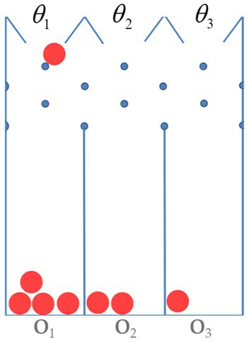
Figure B3.1. A small pachinko game. The figure diagrams a device for a very small pachinko game. Balls can be dropped into one of three slots labeled θ₁, θ₂, and θ₃. Balls fall straight down until they hit a peg. At this they will fall either to the right or the left with equal probability—unless they are against a wall. In this case they will fall inwardly with probability 1. Eventually a ball will enter one of the three bins. These are labeled O₁, O₂, O₃ to indicate outcomes. The slot into which the operator chooses to drop the balls determines the outcome probability distribution.

Table B3.1

Table B3.1. Lists the outcome probability distributions for input slots θ₁, θ₂, and θ₃.

We leave it to the reader to verify these probabilities as an exercise.

The outcome probabilities do depend on the values of θ, nevertheless, one cannot use Bayes’ formula to calculate the conditional probabilities of the θ for several reasons. First, the θ_s are not part of the outcome sample space. And second, the θ_s are fixed and thus do not really have a probability.

Defining likelihood

In formal verbose mathematical notation, the likelihood is defined as: $L\left(\theta ;\mathrm{\hspace{0.33em}}\underset{\_}{x}\right)=C.\mathrm{Pr}\left(\underset{\_}{X}=\underset{\_}{x};\theta \right),$ and should be read as “the likelihood of an unknown but fixed parameter, θ, given an observed/realized vector of observations, $\underset{-}{x}$ is equal to an unknown constant C times the probability that the random variable $\underset{-}{X}$ takes on the value $\underset{-}{x}$ given the parameter $\theta$.”

Likelihoods are not probabilities

The above definition for likelihood was first given by Fisher (1921). In 1921, and for the rest of his life, he was emphatic that likelihood was not a probability. The first thing to notice is that on the left-hand/likelihood side the parameter, $\theta$, is the argument while the observed data. $\underset{-}{x}$, is the fixed conditioning value, but that on the right-hand/probability side the random value, $\underset{-}{X}=\underset{-}{x}$, is the argument while the parameter, $\theta$, is the fixed conditioning value. Thus, we can see from the very structure of the equation that the likelihood is making statements about different values of $\theta$ given the data; probability on the other hand is making statements about different values of X given the parameter.

Other distinctions between Likelihood and probability that Fisher (1921) noted are: First, likelihoods violate Kolmogorov’s rule 3. That is an integral or sum over the argument ($\theta$) does not necessarily equal 1, as it would for a probability. Second, Probability densities change as the way the observations are measured are transformed, such as switch a measurement from inches to miles. In contrast, however you transform a parameter, such as changing the spread parameter from standard deviation to variance, the likelihood remains the same. And third, while probability (or probability density) of a single observation is an interpretable quantity by itself this is not true of the likelihood of a single parameter value because of the unknown constant C. As discussed in the next section, likelihoods can only be interpreted in the comparison of parameter values.

The concepts of probability and likelihood are applicable to two mutually exclusive categories of quantities.

We may discuss the probability of occurrence of quantities which can be observed or deduced from observations, in relation to any hypotheses which may be suggested to explain these observations. We can know nothing of the probability of hypotheses or hypothetical quantities. On the other hand we may ascertain the likelihood of hypotheses and hypothetical quantities by calculation from observations: while to speak of the likelihood (as here defined) of an observable quantity has no meaning (Fisher, 1921).

Fisher felt so strongly about the incommensurability of probability and likelihood as to commit the rhetorical sin of a single sentence paragraph for emphasis. To translate Fisher into the language of this paper, “hypothesis,” “hypothetical quantity,” and “observable quantity” should be interpreted, respectively, as “model,” “parameter value,” and “event.”

Another perhaps even more potent argument that likelihoods should not be thought of as the probability of a model was made later by the statistician Barnard.

To speak of the probability of a hypothesis implies the possibility of an exhaustive enumeration of all possible hypotheses, which implies a degree of rigidity foreign to the true scientific spirit. We should always a“dmit the possibility that our experimental results may be best accounted for by a hypothesis which never entered our own heads (Barnard, 1949).

How likelihood ratio measures evidence

Because the constant C is unknown a single likelihood value cannot be interpreted by itself. However, if a ratio of likelihoods (or equivalently, a difference of log-likelihoods) is formed the constant is eliminated and the ratio is interpretable. For instance, if $\frac{L\left({\theta }_1;\underset{-}{x}\right)}{L\left({\theta }_2;\underset{-}{x}\right)}=16.5$, then one can say that ${\theta }_1$ is 16.5 times as likely as ${\theta }_2$. The likelihood ratio per se does not make a commitment to the truth of either parameter. The likelihood if translated into English is best represented by the subjunctive statement “if the model with parameter ${\theta }_1$ were true, then the probability of the observed data, $\underset{-}{x}$, would be this.” Thus, the likelihood ratio measures the relative plausibility of the two fixed values (see Jerde et al., 2019 for a discussion of the meaning of different magnitudes of the likelihood ratio). The likelihood ratio can be seen as a judicious quantification of the old maxim: where there is smoke there is fire. You could be wrong, because what you think is smoke is actually mist, but comparing the alternatives fire or no fire, if you see smoke, the existence of a fire is definitely more reasonable than no fire.

In our pachinko example, if we observe O₁, then the likelihood ratio for slot 1 vs. slot 2 is (4/8)/(2/8) = 2. There is a small amount of evidence for slot 1 relative to slot 2. If a second ball is dropped and we again observe O₁ then our evidence for slot 1 increases to $\frac{\left(\left(\frac{4}{8}\right)\left(\frac{4}{8}\right)\right)}{\left(\left(\frac{2}{8}\right)\left(\frac{2}{8}\right)\right)}=4$. If more balls are dropped and we observe the sequence {O₁, O₁, O₂, O₁, O₂, O₃, O₁, O₁} then the likelihood ratio is 9 and there is moderate evidence for slot 1 relative to slot 2.

2.1.1 Model/hypothesis

The words “hypothesis” and “model” do not have universally applied meanings, even in otherwise well-defined scientific contexts. Collectively these terms serve two different functions in science and statistics. We sort the functions to the terms to best match common language dictionary definitions.

A hypothesis,¹¹ at least as we construe it is a statement—often verbal, but sometimes mathematical—that can be true or false, at least in principle. A scientific hypothesis contains a provisional explanation of observed facts “written in such a way that it can be proven or disproven” (Grinnell and Strothers, 1988). A model¹² as we use the term is a representation of a phenomenon or process that is capable of producing surrogate data. Models can be physical, such as the miniature wings the Wright brothers ran through their wind tunnel (Wright, 1901), computational (e.g., Gotelli et al., 2009), or analytic (e.g., Dennis and Patil, 1984), see Box 3. A foundational scientific assumption is that models are almost always approximations (Box, 1976), and therefore not strictly true.

2.1.2 Kinds of probabilities

Important distinctions often presuppose still more basic distinctions if they are to be made fundamentally clear. It is a commonplace in introductions of Bayesian statistics for scientists to state that Bayesian statistics uses an interpretation of probability that is distinct from the interpretation of probability used by classical statistics. For instance, Ellison (1986, Table 1) states that the Bayesian interpretation of probability is “The observer’s degree of belief, or the organized appraisal in light of the data,” while the frequentist interpretation of probability is given as a “Result of an infinite series of trials conducted under identical conditions.” This dichotomization of probability is at best a heuristic oversimplification. In our experience, this restriction to only two definitions of probability creates more confusion than it avoids. Two of the named “statistical paradoxes” that we deconstruct result directly or in part result from the failure to distinguish multiple kinds of probability.

This said probability is a very slippery concept. Bell (1945) quotes the great philosopher and mathematician Bertrand Russell as saying in a 1929 lecture “Probability is the most important concept in modern science, especially as nobody has the slightest notion what it means.” For the purposes of this paper, we parse probability into four concepts that are particularly salient for thinking about inference. For clarity, we give each its own individual operator. The kinds of probability we consider are propensity, Pr_p, finite frequency, Pr_f, deductive, Pr_d, and belief, Pr_b.¹³

We observe that in the real world, there is a tendency on the part of objects in standard conditions to behave in routine ways. This natural tendency of objects and conditions is called their “propensity” and has long been characterized as a probability.¹⁴ Notationally, we designate this form of probability as Pr_p. The propensity of a coin to land heads or tails in a particular flipping experiment is exhibited in a sequence of flips. A fair coin might come up heads three times if flipped 10 times, 44 times if flipped 100 times 5,075 times if flipped 10,000 times and 499,669 times if flipped 1,000,000 times.¹⁵ The relative frequency of the occurrence of objects or events in specified populations or conditions is yet another measure of “probability,” and we designate it Pr_f for “finite empirical frequency.” The accuracy of Pr_f as an estimate of the propensity, Pr_p increases with the sample size. We will see later when working with Humphreys’ paradox that propensity is not quite a probability in the strict mathematical sense (see Box 2). It is perhaps better to think of it as the probability generating tendency of the world.

In science, we should always be concerned with the real world and with data. So, what does Pr_d(D), with D standing for data, mean? Well, it actually does not mean anything; only Pr_d(D;M) has meaning. The complete expression, Pr_d(D;M), indicates the frequency with which the data, D, would be generated by the given (fixed; see Box 3) model M in an infinite number of trials (see Box 2).¹⁶ The notation “Pr_d” indicates that the probability has to do with the deductive relationship between models and data and not with an agent’s beliefs. What data could be realized a priori depends on the sort of models proposed. The relationship between a model and its as yet unrealized data is deductive in the sense that M entails the distribution of D for a given specification of M and D.

Let us assume, M₁ says that a flipped coin has a probability of 0.7 to land heads up. Assume further that M₂ says that it has probability 0.6; M₃ says that it has probability 0.4; M₄ says that it has probability 0.3; and so on. Before any actual data have been observed, each of these models tells us how probable any set of observations would be under the model. So, the relationship between models and data distribution is completely deductive, i.e., not in the least dependent on an agent’s beliefs concerning what is the case.

This brings us finally to belief-based probabilities. These are informed by a subjective or psychological understanding of what a “probability” measures. Pr_b(H) is an assessment, on a scale from 0 to 1 of how much the agent believes a hypothesis H to be true. Notice that we have switched the argument of the probability operator/function from data to hypothesis. This is in keeping with our distinction between hypotheses and models, that only hypotheses can be true.¹⁷

2.1.3 Conditioning on either fixed values or random variables

When we introduced deductive probability in section 2.1.2, we noted that the operator “;” should read as “given.” Another reading of “;” is “conditional on.” There is another operator in probability and statistics, the operator “|,” that is also read as either “given” or “conditional on.” The distinction between these two operators is that “;” indicates conditioning on a fixed value, while “|” indicates conditioning on a known realization of a random variable. Conditioning on a fixed value behaves fundamentally differently from conditioning on a random variable. While conditioning on a random variable partitions a predefined sample space (see Box 3), conditioning on a fixed value essentially creates a new space—redefining the probabilities of the primitive outcomes and sometimes even determining the number of outcomes (see Box 3).

2.1.4 Probability/likelihood

Although deeply related and the terms often used interchangeably, probability and likelihood are not the same thing. The first thing to note about this pairing of terms is that the probability being considered is of the deductive kind. Deductive probability is the frequency with which a mechanism will generate events. Likelihood is a measure of the support provided by data for a particular mechanism. This becomes a little bit clearer if one inspects the mathematical definition of likelihood: $L\left(M;D\right)\propto {\mathrm{Pr}}_d\left(D;M\right)$ (Fisher, 1921). This is read as “the likelihood of the model given the data is proportional to the deductive probability of the data given the model.”

On the left-hand-side, the argument of the likelihood function is the model, M (conditional on data D). On the right-hand-side, the argument of the probability function is the data, D (conditional on model M). This change of argument means that the likelihood is about the model while the probability is about the data. Boxes 1 and 2 demonstrate more fully the distinctions between likelihood and probability.

2.1.5 Confirmation/evidence

Words like “confirmation” and “evidence” and slogans like “make only evidence-based or well-confirmed claims” are everywhere in the critical thinking literature, and to the best of our knowledge largely left undefined and interchangeable. In his clear and helpful overview of the topic, Critical Thinking (Haber, 2020),¹⁸ Jonathan Haber uses the word “evidence” at least 30 times without ever attempting to clarify it and conflates rather than contrasts it with “confirmation,” as when he emphasizes “the need to confirm ideas with evidence.” The way these words are generally used clouds rather than clarifies their meanings. To clarify their meanings is in the first place to distinguish them.

On our construal (see Bandyopadhyay and Brittan, 2006; Bandyopadhyay et al., 2016), confirmation and evidence are distinct in so much as confirmation fortifies an agent’s belief that a hypothesis is true as additional data are gathered, while evidence, on the other hand, consists of data more probable on one hypothesis or model than another, or equivalently, one hypothesis or model is more likely than another given the data (see Box 3). That is to say that confirmation is necessarily unitary in that it makes an inference about only one model on the basis of data, but that evidence is necessarily comparative giving the relative support for two or more models on the basis of data.

Consider first the Bayesian account of confirmation. If two random events share a common primitive observation or observations, then the value of one event contains information about the other (see Box 3). A Bayesian agent is interested in what she believes about the truth of hypothesis H conditional on the observation of D. This is written as Pr_b(H|D). The symbol “|” is read as “conditioned on” or “given.” For a Bayesian D confirms H just in case an agent’s prior degree of belief that H is true is raised by the observation of D. The degree to which D confirm H is measured by the extent to which the degree of belief has been raised.

A Bayesian updates beliefs by using Bayes’ rule¹⁹ (see Box 3) that says that the probability of a hypothesis given new data is equal to an agent’s belief that the hypothesis was true prior to having such data, multiplied by the probability of gathering the data on the assumption that the hypothesis is true, divided by the probability of gathering the data averaged over all hypotheses. In symbols,

$\mathrm{Pr}\left(H_{│}D\right)=\mathrm{Pr}\left(H\right)\mathrm{\hspace{0.33em}}\mathrm{x}\mathrm{\hspace{0.33em}}\mathrm{Pr}\left(D_{│}H\right)/\mathrm{Pr}\left(D\right)$

Data confirm a hypothesis just in case the new data increase its probability.²⁰ In symbols, D confirm H just in case Pr(H│D) > Pr(H). Simply put, the Bayesian²¹ learns from experience by raising the probability that their beliefs are true by gathering new data that are in accord with our beliefs (and by lowering the probability if they are not).²²

Evidence on our construal has to do with the relative support given by the data for one model over another model independent of any beliefs an agent or agents may have. The measure of evidence we discuss in this paper is the ratio of likelihoods (see Box 3). If some datum is more probable on one model, rather than another, i.e., makes one model more likely than another, then if gathered is better evidence for the first than for the second. This is to say that data constitute evidence only as they are used to compare pairs of models. Data constitute evidence for one model compared to another just in case the probability of the data on the first model is greater than the data’s probability on the second model. In symbols, when using the Likelihood ratio as the evidence measure:

$E{v}_{LR}\left(M_1;M;D\right)>1\iff \frac{LR\left(M_1;D\right)}{LR\left(M_2;D\right)}=\frac{{\mathrm{Pr}}_d\left(D;M_1\right)}{{\mathrm{Pr}}_d\left(D;M_2\right)}>1$

One way of marking the distinction between the two concepts is to note, following Royall (1997), that confirmation answers the question, “given the data, what should we believe and to what degree?” while evidence answers the very different question, “do the data provide evidence for one model, M₁ against an alternative model M₂, and if so, how much?”

As noted earlier, a foundational scientific assumption is that models are almost always approximations. The concept of evidence as analyzed in this paper reflects this fact. That is, evidence does not necessarily bolster one’s belief that a particular hypothesis/model is true or false; it has to do with showing that one hypothesis/model is better supported by the available data than another. The second distinction follows immediately from the point just made. Evidence compares two models while confirmation adjusts belief in a single model. Data per se are not evidence except insofar as they serve to compare hypotheses, i.e., data constitute evidence only in this sort of multi-model context whereas data confirm hypotheses one at a time.²³

There are at least three key differences between confirmation and evidence. First, confirmation is a measure of the degree to which data raise (or lower) one’s belief that a hypothesis is true, in this sense is agent-dependent, evidence is a measure of the comparative support of two (or more) models on the same set of data, and therefore agent- and truth-independent. Second, since confirmation is characterized in terms of probabilities, its measure must range from 0 to 1. If evidence is measured as an arithmetic ratio between likelihoods, its numeric value can in principle range between 0 and ∞. If evidence is measured as a difference of log-likelihoods its value can range from −∞ to ∞. And third, two agents can reasonably disagree about the degree to which a belief is confirmed if their prior probabilities differ, but no such disagreement is possible in the case of evidence (which is based on nothing more than a logical relation between models and data).²⁴

3 Statistical paradoxes

Paradoxes prompt critical thinking in their resolution, in particular the way in which their resolution often leads to drawing new and significant distinctions. This has been the case in the history of both mathematics and physics, as the examples of Galileo’s Paradoxes of Infinity and Motion (see Box 1) illustrate. However, neither of them is statistical in character. From this point on, the discussion will be focused on some statistical paradoxes and on the distinctions that resolve them in a very fruitful way.

We discuss three statistical paradoxes. In order to make the discussion as clear as possible, in the case of each we first set out the paradox, and then identify a distinction that resolves it, finally indicate how this distinction in turn serves to resolve some public controversies that have an important scientific dimension. In the case of the Lottery Paradox, the discussion is extensive and is intended to provide a model of critical thinking. In the case of the other two statistical paradoxes, the discussion is briefer and intended to reinforce points already made.

3.1 Statistical paradox #1: the lottery paradox

The lottery paradox was first formulated by Kyburg (1961). Suppose a fair lottery with 1,000 tickets. Exactly one ticket will win and, since the lottery is fair, each stands an equal chance of doing so. Consider the hypothesis, “ticket #1 will not win.” This hypothesis has a probability of 0.999. Therefore, we have good reason to believe, and in this sense “accept,” the hypothesis. But the same line of reasoning applies to all of the other tickets. In which case, we should never accept the hypothesis that any one of them will win. But we know, given our original supposition that one of them will win.

This paradoxical result is to be avoided, according to Sober (1963), by denying that we should ever “accept” a hypothesis. Sober uses the lottery paradox to argue for a wholesale rejection of the notion of acceptance. But, of course, this is not the only or, we might add, the most plausible option.

Sober assumes that a hypothesis is acceptable just in case we have very good reason to believe that it is true, i.e., just in case the data support or confirm it to a high degree. But the data that only one ticket will win in a lottery of 1,000 tickets confirms the hypothesis that the first ticket will lose, the second ticket will lose, and so on for all of the tickets. But one ticket is sure to win. A highly confirmed hypothesis that it will lose is false. Therefore, Sober concludes, we should abandon the notion of acceptability, but this, we add, flies in the face of common practice as a result. It should be noted at the outset that lottery generalizations and others of the same kind are unusual in this respect that their truth does not rest on an inference from sampling data, but simply on counting the number of tickets. It can be determined a priori that every ticket has the same probability of winning; in a lottery of 1,000 tickets, the odds of any ticket’s winning are 1/1,000. The point is sometimes made that such generalizations are logically not empirically true.

This point made, three mistakes in the reasoning regarding the Lottery Paradox can be identified. The first mistake is to argue, as Sober does, that if one ticket is sure to win, a highly confirmed hypothesis that it will lose is false. One should note, however, that the probability of a ticket winning is not 0 but 0.001, and the probability of a ticket not winning is not 1 but 0.999. So, while one may have a good reason for believing that an individual ticket will not win, one does not have a good reason for being sure that it will not win.

The second mistake in this treatment of the Lottery Paradox is to treat the drawing of the different tickets as independent. The events are not independent if they were generated by a lottery. If a ticket is a winner, then no other ticket can be a winner. If a particular ticket is not a winner, then the probability of any other ticket being the winner increases because the winning ticket is now one ticket out of a pool of tickets whose number has decreased by 1. From these simple observations, we can build an induction that rejects the conclusion that there is no reason to believe that any ticket will win the lottery.

Say we have purchased all 1,000 lottery tickets and lined them up on the edge of a table. We can ask what the probability is that the first ticket is not the winner. We know from the rules of this lottery that there are 1,000 tickets and 999 of them are not winners, thus from the rules of probability (see Box 2) the probability that the first ticket is not the winner is 999/1,000. Now let us ask “what is the probability that the winning ticket is not in the first two tickets.” This probability is the probability the first ticket is not the winner times the probability that the second ticket is not the winner (given that first ticket was not the winner) that is (999/1,000) (998/999). The probability that the winner is not in the first three tickets is the probability that it is not in the first two tickets multiplied by an even smaller number (997/998).

The multiplier for the ith ticket is (1,000−i)/(1,001−i). The multiplier for the 1,000th ticket is 0. Thus, we know to a certainty that if these tickets came from a true lottery of 1,000 tickets that the set of all tickets will contain the winner.

To round out this critical analysis, we point out that the sense of paradox engendered by the lottery paradox is based on an implicit equivocation: the statement that “no single ticket is likely to be a winner” is not at all the same as “not one ticket is likely to be a winner.”

In deflating the lottery paradox, we have employed all three methods in List 1. First, we rejected the premise that a low probability of something being true is a good reason for believing that it is not true. Second, we modified (corrected) a premise on how to combine discrete hypotheses into composite hypotheses. And third, we have pointed out an equivocation in the statement of the lottery paradox.

This way out of the lottery paradox is successful and relatively straightforward. The distinction that it draws between “no single ticket is likely to be a winner” and “not one ticket is likely to be a winner” is both fundamental and widely applicable.²⁵ Moreover, failure to make the distinction rests on not taking the prior probability of winning or not winning the lottery given the number of tickets sold into account, a basic element in any Bayesian calculation of the odds of holding the winning ticket. But another equally successful way of resolving the Lottery Paradox is perhaps more intuitive and it rests on a distinction that is directly relevant to an analysis of the concept of evidence.

On Sober’s formulation of the Lottery Paradox, a hypothesis is acceptable just in case we have very good reason to believe that it is true, i.e., it is well confirmed. We have very good reason to believe of every ticket that it will lose. Therefore, the generalization is acceptable. But one ticket will win. Paradox. But if every ticket is just as likely to be the winner as every other ticket, then there is no evidence that any one of them will win or lose. If we maintain that a hypothesis is acceptable only if it is both well confirmed and there is evidence for it, then the hypothesis that every ticket will lose is not acceptable. Paradox lost.

3.2 Statistical paradox #2: the old evidence paradox

The old evidence paradox can be resolved in the same illuminating way as the lottery paradox, by making a distinction between the probability of the data and the probability of the data given a model. It is not a paradox for statistical inference generally, but only for the Bayesian account of inference. At the same time, however, its resolution helps to reinforce and throw further light on our analysis of the evidence concept. The classic formulation of the paradox is due to Clark Glymour.²⁶ Before analyzing the paradox, we need to point out that the word “evidence” in the name of the paradox is used in sense of “data,” or “information,” or simply something that helps confirm a hypothesis—not in the model comparison sense we have introduced above.

In the actual practice of science, often models come to be accepted not because they yield novel predictions that are subsequently verified, but because they account more successfully than competing models for observations previously made. Copernicus’ heliocentric theory was supported with observations dating back to Ptolemy. The theory of universal gravitation was supported by Newton’s derivation of the laws of planetary motion that had already been established empirically by Kepler.

But Glymour (1980) and others contend that this sort of “old” data apparently does not confirm new hypotheses. Glymour argues from the fact that in cases of “old” data “the conditional probability of T [i.e., the theory or hypothesis] on e [the datum] is therefore the same as the prior probability of T” to the conclusion that “e cannot constitute evidence for T.” This analysis makes hash of the history of science and of ordinary intuition, which is why Glymour dubbed it a paradox.

For clarity, translating this into the notation of this paper: If data D are already known when hypothesis H is introduced at time t then Pr(D) = 1. Consequently, the probability of D given H, Pr(D│H) must also equal 1. Thus, by Bayes’ rule, Pr(H│D) = Pr(H) x 1/1 = Pr(H). That is, the posterior probability of H given D is the same as the prior probability of H; D does not raise its posterior probability, hence, contrary to practice and intuition, does not confirm it.

This analysis fails to take into consideration both the distinction between a random variable and a realization of the random variable (see Box 2) and the distinction between the probability of an observation and the probability of an observation under a model (see Box 3). A random variable can be defined “as a variable that takes on its numerical values by chance.” A realization is an observation of one of those chance values. Part of the philosophical confusion embodied in the old evidence problem stems from conflating “knowing or observing the data” with “the probability of the data.” More important is the misunderstanding of Pr(D│H). This probability is a deductive consequence of the model/hypothesis. For this reason, in section 2.1.2, we suggested denoting it as Pr_d(D│H). But regardless of the notation, even in a subjective Bayesian analysis, the probability of the data given the model cannot be adjusted but must be accepted as a belief based on a contingent fact (Lewis, 1980).

It should be clear how the old evidence paradox rests both on a failure to distinguish “evidence” from “confirmation” typical of philosophical work on the topic of confirmation generally and the failure to distinguish Pr_b(D) (which given observation of D is 1) from Pr_d(D; M) (which is independent of whether the D is observed or not). On the generally Bayesian account D is evidence for H if and only if Pr(H│D) > Pr(H), where the latter probability is just an ideal agent’s current probability distribution. Once this conflation is undone, by distinguishing sharply between evidence and confirmation, then so too is the paradox. For this conclusion can now be seen to be a non-sequitur. “Old” evidence or new, data is data and provides fuel for confirmation.²⁷

Perhaps the most celebrated case in the history of science in which old data have been used to vindicate a theory concerns the perihelion shift (S) of the planet Mercury and the General Theory of Relativity. Of the three classical tests of GTR, S is regarded as providing the best evidence.²⁸ According to Glymour, however, a Bayesian account fails to explain why S should be regarded as evidence for GTR. For Einstein, Pr(S) = 1, since S was known to be an anomaly for Newton’s theory long before GTR came into being.²⁹ Einstein derived S from GTR. Therefore, Pr (S│GTR) _≈ 1. Once again, since the conditional probability of GTR given S is the same as the prior probability of GTR, it follows that S cannot constitute evidence for GTR. But given the crucial importance of S in the acceptance of GTR, this is at the very least paradoxical.³⁰

On our Evidentialist account, however, S does constitute evidence, indeed, very significant evidence. Consider GTR and Newton’s theory, NT, relative to S with different auxiliary assumptions for the two theories. Two reasonable background assumptions for GTR are (i) the mass of the Earth is small in comparison with that of the Sun, so that the Earth can be treated as a test body in the Sun’s gravitational field, and (ii) the effects of the other planets on the Earth’s orbit are negligible. Let A_E represent those assumptions.

For Newton, the auxiliary assumption is that there are no masses other than the known planets that could account for the perihelion shift. Let A_N stand for Newton’s assumption. We now apply our evidential criterion, the Likelihood Ratio, to a comparison of the two theories, albeit in a very schematic way. Pr(S│GTR & AE) ≈ 1, whereas Pr(S│NT & AN) ≈ 0. The LR between the two theories on the data goes approaches infinity, which is to say that S provides a very great deal of evidence indeed for GTR and virtually none for Newton’s theory.³¹

Glymour advanced the OEP as the principal reason why he was not a Bayesian.³² But it is neither necessary nor advisable to reject Bayesianism out of hand, only to assign it its proper roles. These latter include among many applications, the estimation of parameters and as in this paper, its account of confirmation. A good case can be made that a hypothesis or model is scientifically “acceptable” just in case it is both well confirmed and supported by strong evidence.³³ Evidence in itself is not a decision rule, nor is it a confirmation measure. It seems perfectly reasonable for a scientist or a community of scientists to continue to probe a model evidentially, by compiling more data, or by comparing the original model with new models until the community is satisfied. Moreover, while the testing of models and the measurement of the evidence for and against them are best understood in terms of their respective likelihood ratios, the Bayesian account of the basis on which to choose the models to test is very plausible, having to do as it does with choices made by individual scientists.

3.3 Statistical paradox #3: Humphreys’ paradox

Humphreys’ paradox (HP) questions the probabilistic nature of propensity. Although the statement and analysis of HP was originally quite technical its gist can be simply stated. Humphrey (1985) noticed that if propensity is considered as a conditional probability, i.e., Pr_p(D|C), where D is some observed event and C is the conditioning event, no matter how one twists and turns some contradiction occurs (Humphreys, 1985, 2004). The most fundamental of these is a violation of time irreversibility. An application of Bayes’ theorem (see section 2.1.5 and Boxes 2 and 3) indicates that data (observed after the fact) can influence the conditioning event.

The HP has withstood decades of critical analysis.³⁴ The conclusion is consistent: Whatever propensity is, it cannot be expressed as Pr_p(D|C). In section 2.1.3 and in Boxes 2, 3, we distinguished two kinds of conditioning that occur in statistics and stochastic processes. One can condition on a random variable, or one can condition on a fixed effect. Conditioning on a random variable (B) restricts to a subset of the sample space that the probability of the event A is being calculated over. Likewise conditioning on A restricts to a subset the sample space that the probability of B is being calculated over. However, if one conditions on a fixed value B, the value of random variable A has no effect on the fixed value because it is well fixed. The rules of probability that Humphreys (1985) found violated involve conditioning on random variables.

Considering propensity as a random distribution conditioned on fixed values (i.e., generating conditions or states) dissolves Humphreys’ paradox (Ballantine, 2016). When thinking about Humphreys’ paradox, it is important to realize that while the propensity is a property of the generating conditions, the generating conditions are not a property of the propensity. Different generating conditions may induce the same propensity.

Early 20th-century statisticians, scientists, and philosophers took the lesson from Hume that since cause was not knowable it should not be studied. Increasingly since the late 20th century scientists, statisticians, and philosophers have come to recognize that while mechanism may not be knowable, it is a reasonable object, and perhaps one of the primary goals of scientific study. What is revelatory in this analysis of the HP is the weakness of Bayesian methods in the pursuit of mechanism that is propensity. Bayesian analysis depends on Bayes’ rule. Which depends on conditioning on random variables. Bayes rule is a valid tool when conditioning on random variables but not when conditioning on fixed conditions (Pearl, 2000; Ballantine, 2016) in the same way that Euclid’s theorems hold for objects on a plane, but not unmodified for objects on a curved surface. The study of the partitioning of sample spaces by random variables is the study of correlations, or more generally statistical dependence. In Box 3, we show that Bayes’ rule can be written in terms of the correlation between random variables, whether discrete, continuous, or mixed.

It is natural to assume that the tendency of a model to generate a particular sort or set of data represents a causal tendency on the part of natural objects represented in the model to have particular properties or behavioral patterns. This tendency or “causal power” can be both represented and sometimes explained by a corresponding model. In our view, a fully objective account of evidence requires that we must make this realist assumption and thus take model probabilities as modeled propensities. Thus, the distinctions we have drawn among the four kinds of probabilities greatly clarify how probability can be used to learn about both pattern and process in science (see Figure 1).

Figure 1

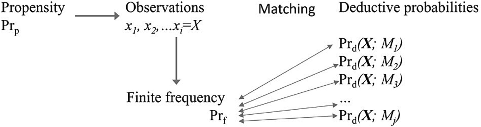
Figure 1. Schematic representation for the relationships among kinds of probabilities in a statistical inference. In subjective Bayesian statistics, matching is measured by degrees of belief using Bayes formula. In likelihood or evidential statistics, matching is measured through evidence (see Box 3).

Humphreys’ paradox, on the other hand, indicates both that propensity needs to be somehow differentiated from other kinds of probabilities and that the rules of probability (at least as stated by Kolmogorov, 1956) do not quite apply to propensity.

Probabilities, and their partitioning by Bayes’ rule are static (see Box 2), but propensities are dynamic. Propensities generate probabilities depending on the full set of conditions impinging at a given time. This leads us to the realization that the conditions at one time probilistically cause the conditions at a second time, which in turn probabilistically cause the conditions at a third time.³⁵ Probability theory by itself cannot elucidate causation because probabilities are invertable (see Box 2) and causation is not.

The great geneticist Sewall Wright had the spectacular insight that one can predict the correlations among variables that would develop under an assumed causal model. Or conversely, one could estimate the magnitude of causal effects from observed correlations and an assumed schema of causal interactions.

But it would often be desirable to use a method of analysis by which the knowledge that we have in regard to causal relations may be combined with the knowledge of the degree of relationship furnished by the coefficients of correlation. […] In a rough way, at least, it is easy to see why these variables are correlated with each other. These relations can be represented conveniently in a diagram like that in figure r, in which the paths of influence are shown by arrows (Wright, 1921).

It is the arrows in path analysis that capture the non-invertibility of propensity correctly. Modern descendants of path analysis include structural equation modeling (Bollen, 1989) and do-calculus (Pearl, 2000). Much of both the statistical and the pragmatic scientific literature has disparaged all varieties of causal analysis because the necessarily assumed causal models cannot be proved (Denis and Legerski, 2006).

But with an evidential analysis models are not proved, disproved or confirmed. Alternative models are compared by the degree to which they can approximate real data. Alternative causal models can be compared to each other and even with non-causal models (Taper and Gogan, 2002; Taper et al., 2021).

In summary, the resolution of Humphrey’s paradox is to recognize that Humphrey was right. Propensity/cause cannot be characterized fully by probability. However, because propensity is probability generating it can be inserted into statistical analysis point wise and studied using deductive probabilities. The facts that the causal models must be assumed a priori and that the models are almost surely not true but only approximations do not block statistical inference but do suggest the comparative approach of evidential statistics may be more fruitful than either Bayesian analysis or classical hypothesis testing.³⁶

4 Distinction making in real science

4.1 COVID

An example of weak confirmation and strong evidence with widespread implications has to do with the “base-rate fallacy” which infects most people’s uncritical thinking.³⁷ The example has to do with the much-circulated claim that vaccines are ineffective in preventing COVID-related infection/hospitalization/death. This claim rested on correlations between, e.g., COVID-related death rates and vaccination status.

The U.S. Centers for Disease Control and Prevention … compared data from 28 geographically representative state and local health departments that keep track of COVID death rates among people 12 and older in relation to their vaccination status, including whether or not they got a booster dose, and age group. Each week in March, on average, a reported 644 people in this data set died of COVID. Of them, 261 were vaccinated with either just a primary round of shots – two doses of an mRNA vaccine or a single dose of Johnson and Johnson’s vaccine -or with that primary series and at least one shot of a booster (Montañez and Lewis, 2022).

These numbers appear to indicate that roughly 40% of those vaccinated died anyway, in which case the shots were not much better than marginally effective. What was not taken into account, however, was the fact that the vaccinated or boosted population was much greater, 127 million, than the unvaccinated, 38 million. A much smaller fraction of vaccinated or boosted people are likely to die from the disease, but since there are many more of them, the total number of deaths among the vaccinated will approach and if sufficiently large surpass the number among the unvaccinated.

This is an instance of the “base-rate fallacy” neglecting to take into account the relative frequency with which a particular property, in this case being vaccinated, occurs in a given population, in this case living in the United States. Once the fact that a sizable majority of the people in this country have been vaccinated is taken into account and the relative mortality rates adjusted, it is clear that they are much less likely to die from COVID infections. Given that no more than 60% of those sampled in a given week survived, the effectiveness of vaccination seems weak. But as soon as the number of those vaccinated is considered, it is clear that there is ample evidence for vaccine effectiveness.

Another way to underline the disparity between the mortality rates of the vaccinated and unvaccinated, and to connect the importance of the base-rate to the distinction between confirmation and evidence,³⁸ is to focus on incidence rates, e.g., the number of deaths per 100,000 people per week. Among the unvaccinated in March of 2022, it was 1.71, among the vaccinated 0.22, among the vaccinated and boosted 0.1. That the death rate was so low among the unvaccinated led many people to simply shrug off the need to visit their pharmacist. But it also entails that the degree to which the efficacy of vaccination is confirmed is very weak, the result of taking the base-rate into consideration as the prior probability in a Bayesian calculation. Note, however, that on the basis of their respective incidence rates an unvaccinated person is 7.7 times more likely to die than a vaccinated, 17.1 times more likely to die than someone who has also received a booster shot.³⁹ This is, moreover, just what the calculation of evidence reveals, that the ratio of mortality rates in the first case is 7.7, in the second 17.1, i.e., that the preponderance of evidence supports the efficacy of vaccination, especially when boosted. A large number of retrospective analyses have calculated that vaccinations make a large difference in the real world. For example, Steele et al. (2022) calculated that in just the first 10 months after vaccines became available about 235,000 lives were saved due to vaccination. This is a rather dramatic public policy demonstration of the fact that confirmation needs to be distinguished from evidence and that evidential considerations are crucial when public policy decisions are being made.

4.2 Climate change

In our discussion of the effectiveness of COVID vaccines above, we made clear how assimilating confirmation and evidence is a potential source of the base-rate fallacy and in turn how the distinction between them makes vivid the strength of the claims for the effectiveness of the vaccines. Another example, already mentioned in connection with the failure of public opinion to align with scientific consensus, concerns the hypothesis that global climate change, together with its deep and widespread impact on our planet’s plant and animal life, is mainly the result of human activities, burning carbon-emitting fossil fuel for energy in particular. We discuss this example in some detail, not only to underline the importance of the distinction between confirmation and evidence to resolving at least some of the controversy surrounding it, but also to extend our discussion of COVID vaccines by showing how the distinction can be used to demonstrate the difference between correlation and causation. This second difference is as critical to critical thinking as the first, and what we take to be a more or less general failure to take them seriously in dealing with large-scale policy and implementation questions is, at least in our view, only too evident. The second example calls for a more detailed discussion than did the first. The COVID vaccination controversy is, we hope, short-term. The climate change controversy has been with us for decades. Coming to terms with the arguments on each side involves making more than one distinction.

Simply put, the climate change hypothesis is that present and accelerating warming trends are human induced (“anthropogenic”). A wide spectrum of data raises the posterior probability of the hypothesis, in which case they confirm it. Indeed, in the view of virtually all climatologists, this probability is very high. The Inter-governmental Panel on Climate Change contends that most of the observed temperature increase since the middle of the 20th century has been caused by increasing concentrations of greenhouse gases resulting from human activity such as fossil fuel burning and deforestation. In part, this is because the reasonable prior belief probability that global warming is human induced is very high. It is assigned not on the basis of observed relative frequencies so much as on the explanatory power of the models linking human activity to the “greenhouse effect,” and thence to rising temperatures. In part, the posterior probability of the hypothesis is even higher because there are so many strong correlations in the data. Not only is there a strong hypothesized mechanism for relating greenhouse gases to global warming, but also this mechanism has been validated in detail by physical chemistry experiments on a micro scale, and as already indicated there is a manifold correlation history between estimated CO₂ levels and estimated global temperatures.

Some climate sceptics question these conclusions. The main skeptical lines of argument are that (a) the probability of the data on the alternative default (certainly simpler) hypothesis, that past and present warming is part of an otherwise “natural” and long-term trend, and therefore not “anthropogenic” is just as great, (b) that the data are at least as probable on other, very different hypotheses, among which solar radiation and volcanic eruption, and (c) that not enough alternative hypotheses have been considered to account for the data. That is, among credible climate skeptics there is some willingness to concede that burning fossil fuels leads to CO₂ accumulation in the atmosphere and that carbon dioxide is a greenhouse gas that traps heat before it can escape into the atmosphere, and that there are some data correlating a rise in surface temperatures with CO₂ accumulation. But, the skeptics continue, these correlations do not “support,” let alone “prove,” the anthropogenic hypothesis because they can be equally well accounted for on the default, “natural variation” hypothesis or by some specific alternative. But this conclusion rests on a conflation of evidence with confirmation and provides a striking reason why it is necessary to distinguish the two.

Even the NASA Global Climate Change website under the heading “How Do We Know Climate Change is Real?” embeds the confusion. The website lists four “takeaways,” the main premises in the argument for anthropogenic climate change:

1 “While Earth’s climate has changed throughout its history, the current warming is happening at a rate not seen in the past 10,000 years.”

2 “According to the Intergovernmental Panel on Climate Change (IPCC), ‘Since systematic scientific assessments began in the 1970s,’ the influence of human activity on the warming of the climate system has evolved from theory to established fact.”

3 “Scientific information taken from natural sources (such as ice cores, rocks, and tree rings) and from modern equipment (like satellites and instruments) all show the signs of a changing climate.”

4 “From global temperature rise to melting ice sheets, the evidence of a warming planet abounds.”

But (1) rests on the high correlation between the rates of fossil fuel emissions and globally averaged temperature increases and offers no further reason for thinking they are causally connected, (2) is an argument from authority and, however respected the membership of the IPCC, forestalls rather than invites critical thinking on the part of the under-informed public, everyone grants that (3) is true, i.e., that the climate is indeed changing (when the question is why), and (4) once again provides no reason to think that climate change is wholly or even significantly caused by human activities.

To be clear, the facts alluded to in (1), (3), and (4). all provide excellent reasons for believing that global warming is both real and rapid, a high degree of confirmation. But they do not disarm the sceptics who insist on evidence for the claim that it is human caused as opposed to a natural trend.

Data are evidentially relevant only if they discriminate among hypotheses, and such data in the case of human-induced warming are rarely mentioned. But they are available.⁴⁰ There are three isotopes of carbon atoms, each with a different mass—carbon-14 (¹⁴C) the heaviest, carbon-13 (¹³C), and carbon-12 (¹²C), the lightest and most common. All three are present in CO₂ molecules. Their relative proportion in the sources and sinks of CO₂ varies. Briefly, “the smaller the [change in the percentage of a] ¹⁴C value in a measured sample, the fewer ¹⁴C atoms in it, and the more of its carbon dioxide is from fossil fuel emissions,” therefore the percentage of atmospheric CO₂ that comes from fossil fuel emissions is increasing. In particular, if the CO₂ atmosphere comes from the surface (and not the depths) of the ocean, then ¹³CO₂ will increase over time. If the CO₂ comes from fossil fuel burning, then the relative abundance of ¹³CO₂ to ¹²CO₂ will decrease. Experimental results show that while CO₂ concentration is increasing the ¹³CO₂/¹²CO₂ ratio is decreasing. Because a decreasing ¹³CO₂/¹²CO₂ ratio is much more probable under the anthropogenic model than the surface water model, the observed decrease is evidence for the hypothesis that fossil fuels rather than surface water are mainly responsible for rising levels of CO₂ in the atmosphere, and hence (on the assumption that rising levels of CO₂ are a cause of rising temperatures) for the anthropogenic hypothesis. Isotopes are often described as “fingerprints;” in the case of climate change as commonly in court proceedings they provide excellent evidence of the culprit’s identity and guilt.

Does critical thinking about climate change require digging into the isotopic evidence? Not in general. But here as everywhere it requires at least raising the question: are there data on the basis of which we can compare the anthropogenic model with one or more of its “natural cause” alternatives and determine in a precise way whether it is more likely on these data than the others? As noted at the outset, discussions of “critical thinking” invariably insist that among other things it is “evidence-based.” But “evidence” must be characterized more carefully as we have here before it has any real bite, one that is capable of distinguishing generally between various models all of which are consistent with or can be correlated with the data.

If that distinction is not made, then neither is the case for human-caused climate change. But of equally great inferential import, neither can a distinction be made between correlation and causation. The correlation of the data with the predictions of a model, however close, does not by itself entail whether the variable identified in the model was causally responsible for the occurrence of the data unless other variables that might have been responsible for the occurrence of the data can be ruled out. This is often put by saying that correlation per se does not rule out the possibility of alternative models that explain the data better.

5 Context and coda

A major premise of this paper is that while universally lauded, “critical thinking” is so generally characterized as to provide little direction for those who wish to engage in it. The great American philosopher Dewey (1910), sometimes held to be “the father of contemporary critical thinking,” wrote that it entailed “active, persistent, and careful consideration of a belief or supposed form of knowledge in the light of grounds which support it and further conclusions to which it tends.” “The grounds which support it” may be taken as roughly synonymous with “evidence.” Virtually every discussion of critical thinking with which we are familiar invokes the term and leaves it at that. Our effort here has been to analyze it in enough detail to extract some relatively uncomplicated ways in which to understand and apply it.

The analysis has two principal components: that evidence best understood involves the comparison of two or more models and that the most efficient and in our view, intuitive way to compare them is in terms of their respective expected likelihood ratios.

A geologist, Chamberlin (1900), introduced the necessity of multiple working hypotheses in 1890, in large part to curb a natural tendency to “press a theory to make it fit the facts and a pressing of the facts to make them fit the theory.” When the theory is our own, we today call this “confirmation bias.” Chamberlin (1900) thought that the practice of simultaneously entertaining several working hypotheses, “when faithfully followed for a sufficient time, it develops a mode of thought of its own kind which may be designated the habit of complex thought…” which mitigates confirmation bias.

Although the multiple method was and continues to be standard in, among other sciences, physics and chemistry—the comparison of the GTR with the Newtonian calculation of planetary orbits by way of more precise measurements of perturbations in the orbit of Mercury is a paradigm example—it was neglected in biology, psychology and other more “observational” sciences. With this in mind, the physicist/biophysicist, Platt, published an article in 1964 on “Strong Inference,” reviving and extending Chamberlin’s line of thought. It consisted of “applying the following steps to every problem in science…”

1 Devising alternative hypotheses.

2 Devising a crucial experiment (or several of them), with alternative possible outcomes, each of which will, as nearly as possible, exclude one or more of the hypotheses.

3 Carrying out the experiment so as to get a clean result.

(Recycling the procedure, making subhypotheses or sequential hypotheses to refine the possibilities; and so on).

Platt thought that if these steps were rigorously followed, not only would bias be curbed but much more “rapid and powerful progress would be made” (as in physics).

Although Platt’s article was much celebrated,⁴¹ it failed to alter the conduct of hypothesis or model testing in biology and the social sciences in a mainstream way. In a 2017 article, “Why are we not evaluating multiple competing hypotheses in ecology and evolution, Betini et al. (2017), found that “Only 21 of 100 randomly selected studies from the ecological and evolutionary literature tested more than one hypothesis and only eight tested more than two hypotheses.” He and his colleagues then went on to list three forms of cognitive bias – confirmation, pattern seeking, and belief⁴²—that the multiple hypothesis method would eliminate and identify several intellectual and practical barriers that discourage scientists from using it more widely. Among other points made is that the method not simply encourages but enforces more creative thinking in coming up with alternative hypotheses and models.⁴³ In this respect, no sharp distinction between “critical” and “creative” thinking should be made.

But there is a difficulty with “strong inference” as outlined above, viz., that on it “crucial experiments” are possible that lead to the “exclusion” of one or more of the hypotheses under consideration. This is often but not always the case, and rarely so when the hypotheses are statistical in character or their claims established on the basis of statistical inferences. In this increasingly common sort of case, it is not so much a question of excluding one or more hypotheses or models as of weighing the evidence for one as against the other(s). This is the second component of our analysis of evidence: a way to compare alternative hypotheses that avoids the inappropriately binary “accepted”/“excluded.” As the papers cited all admit, to this point in time no hypothesis in any science has been permanently “accepted” or “included”; rather, we would say, there is at any point in time more evidence in support of one than of the others. There are a variety of ways in which to measure the evidential support of one hypothesis or model as against another. For a number of reasons given in the body of this paper, we favor likelihood ratios.

Chamberlin and Platt urge several critical-thinking “habits” of mind. We recommend that the following be included among them.

List 3: Healthy habits of mind:

1 Wherever possible test alternative hypotheses/models. It is likely that there is a better alternative to the one you have already decided to test.

2 Weigh the evidence for and against hypotheses and models using evidence measures such as the likelihood ratio. Remember that it is always with respect to particular datasets.

3 Distinguish evidence and confirmation and recognize the different roles that each plays. In the process, abandon uniform adherence to one statistical paradigm—Bayesian or Likelihoodist, for example. Different problems require different paradigms for their solution.

4 Remember that making an adequate distinction is often the best way to think critically about a problem. Let it become a habit.

5 At least from time to time, ponder a paradox.

Data availability statement

The original contributions presented in the study are included in the article/supplementary material, further inquiries can be directed to the corresponding author.

Author contributions

GB and MT have contributed equally to the article’s conceptualization and writing. All authors contributed to the article and approved the submitted version.

Funding

Funding of publication cost was provided by the Montana State University Library.

Acknowledgments

This manuscript was greatly improved by the informed and useful comments of Prasanta S. Bandyopadhyay, Brian Dennis, Christopher L. Jerde, Subhash R. Lele, José M. Ponciano, and Preston Stovall, our editor and two reviewers. As we disagree in some points with each, we accept all remaining errors in the manuscript as our own.

Conflict of interest

The authors declare that the research was conducted in the absence of any commercial or financial relationships that could be construed as a potential conflict of interest.

Publisher’s note

All claims expressed in this article are solely those of the authors and do not necessarily represent those of their affiliated organizations, or those of the publisher, the editors and the reviewers. Any product that may be evaluated in this article, or claim that may be made by its manufacturer, is not guaranteed or endorsed by the publisher.

Footnotes

1. ^In 1990, for a typical example, “The American Philosophical Association convened an authoritative panel of 46 noted experts on the subject to produce a definitive account of the concept. It resulted in the production of the landmark Delphi Report. This led to the following definition of critical thinking: (Davies, 2015).We understand critical thinking to be purposeful, self-regulatory judgment which results in interpretation, analysis, evaluation and inference as well as explanation of the evidential, conceptual, methodological, criteriological, or contextual considerations upon which that judgment was based. Critical thinking is essential as a tool of inquiry. Critical thinking is a pervasive and self-rectifying, human phenomenon. The ideal critical thinker is habitually inquisitive, well-informed, honest in facing personal biases, prudent in making judgments, willing to consider, clear about issues, orderly in complex matters, diligent in seeking relevant information, reasonable in selection of criteria, focused on inquiry and persistent in seeking results which are as precise as the subject and circumstances of inquiry permit (Davies, 2015).But this sort of vague “definition,” common in the literature, is of little help. What is it, for example, to be “prudent” in making judgments?

2. ^The widely cited work of the psychologist Stephen Landowsky is typical. In (2020), for example, he urges us to “re-store the pursuit of evidence-based truth as a consensual feature of democratic societies” without indicating what evidence-based truth involves or how it is to be recognized, apparent presuppositions of its restoration.

3. ^There are three leading inferential approaches in science: classical frequentist error statistics, Bayesian statistics, and likelihood/evidential statistics. Descriptions of and comparisons between them can be found in Barnett (1999), Lewin-Koh and Taper (2004), and Taper and Ponciano (2016). Since the contrast between their approaches better serves the points we want to make in this paper, we have centered the discussion on the second and third. Dennis et al. (2019) is a paper that contrasts the efficacy of classical error statistics with that of evidential statistics.

4. ^To gather expert-based judgments on an issue is the so-called “Delphi Technique” pioneered by the Rand Corporation in the 1950s (see Dalkey and Helmer, 1963) and “used internationally to investigate a wide variety of issues” (Niederberger and Spranger, 2020, p. 1). The technique was used to produce the Delphi Report quoted in footnote 1. It is also much criticized. In intervention research in health sciences, for example, surveys of experts are considered subordinate to evidence-based methods because they do not take account of reliable findings on observed cause-effect relationships (see Bodedeker and Backhaus, 2010) and cannot be assigned to any specific methodological paradigm (Niederberger and Springar, 2020, and the variety of sources they cite).

5. ^Although the many studies on which Landowsky draws are for the most part statistical in character, his emphasis is on what is true and false, not on what is more or less likely. Although the social media and political contexts he signals out should often be ignored, we are not told in any direct way how to recognize what is false. Instead, we are apparently to trust the published studies that identify misinformation and suspect any claim that is advanced with a great deal of surrounding “noise.”

6. ^This is not to mention the vast extent to which commercial advertising incorporates and depends for its effectiveness on consumer surveys, product comparisons, and at least alleged scientific studies. Without any tools in hand with which to assess their reliability, we are left to accept or reject them at face value.

7. ^As Niederberger and Spranger (2020) put it, “From a sociological perspective, these techniques raise questions about their validity, the dominance of possible thought collectives, and the reproduction of possible power structures” (see also Scheele, 2002).

8. ^An examination of a randomized 3,000 paper subset of 88,125 English-language climate change papers.

9. ^A figure in line with the Pew Research Center and other recognized polling organizations.

10. ^Among the myriad examples of how this traditional distinction is made and applied, see Doezma and Hauswald (2002).

11. ^Cambridge Dictionary: “an idea or explanation for something that is based on known facts but has not yet been proved.”

12. ^American Heritage Dictionary: “A schematic description or representation of something, especially a system or phenomenon, that accounts for its properties and is used to study its characteristics.”

13. ^A note on nomenclature: propensity, finite frequency, and deductive probabilities are all often referred to as aleatory probabilities, where aleatory refers to probabilities deriving from natural randomness. Belief probabilities are often called credal, subjective, epistemic, or even evidential probabilities. Our definition of deductive probability subsumes much of what are known as classical or logical probabilities.

14. ^For example, by Peirce (1878).

15. ^Numbers of heads at the various sample sizes generated by the rbinom function in the program R version 4.1.0. If the model is physical or a simulation, then Pr_d(D;M) can be estimated by repeating the experiment (see Box 2) a large number of times.

16. ^If the model is physical or a simulation, then Pr_d(D;M) can be estimated by repeating the experiment (see Box 2) a large number of times.

17. ^Much of the literature using belief probabilities, particularly in philosophy, uses H as the argument.

18. ^Haber, like so many others, associates critical thinking to a large, although not complete, extent with the types of reasoning characteristic of Western science, one reason for taking a closer look at the structure of scientific, hence statistical inferences.

19. ^After the 18th century clergyman Thomas Bayes (1702-1761) who first derived it from the rules basic of conditional probability (see Box 2). In our view, “basic Bayesianism” is at once a theoretical perspective that accords special importance to Bayes’ rule in the confirmation and acceptance of theories, a particular interpretation of the probabilities in that rule in terms of the strength of beliefs that certain hypotheses are true/false, and a description of how rational agents both do and should strengthen or weaken their beliefs on the basis of accumulating data. Bayes’ “theorem” is just that, a derivation from the axioms/rules of probability theory and the definition of conditional probability. It takes the form of a methodological paradigm only with a belief-interpretation of the probability operators within it and its consequent application to the strengthening/weakening of beliefs on the part of individual agents. There are any number of variants on this basic theme. Good (1971) estimated that there are, at a minimum, 46,556 possible interpretations of the Bayesian position (to which he added, “more possible interpretations than there are statisticians”). We’ve settled for what might be taken as “the core” of the Bayesian position explicit in such classic formulations as (De Finetti, 1937), without presuming to judge whether it is the “correct” or “true” account of it. There are none such. Moreover, as is made explicit in the final section of this paper, our position is not that the Bayesian paradigm is “mistaken,” but that like the other major statistical paradigms should be understood to apply to the solution of some methodological questions (e.g., hypothesis confirmation and personal belief adjustment, but not all methodological questions).

20. ^Prob(H│D) is called the posterior probability of H, Prob(H) the prior probability of H, Pr(D│H) the probability of D conditional on H, and Pr(D) the expectedness of D. Data confirm a hypothesis when the posterior probability is greater than the prior probability. Many Bayesians, even such excellent ones as Kass and Raftery (1995) refer to Pr(D|H) as a likelihood. As discussed in Box 3—it is not a likelihood as defined by Fisher. The likelihood is ∝Pr(D;H). For Bayesians H is a random variable so the bar notation is appropriate, but that does not make it a likelihood.

21. ^Bayesianism has many variations. Some contemporary Bayesians distinguish between “actual analysis” and “Bayesian epistemology” and a reviewer of our paper has asked us to make both this and the fact that we are doing the latter, not the former clear. Here, in part is what we (Brittan and Bandyopadhyay, 2019) have written about this distinction in the past. Contemporary Bayesianism is ostensibly superior to its unacceptably “subjective” original by way of restricting allowable priors (see, e.g., Clark, 2005). It is often held to be similarly superior to likelihoodism in its apparently unique ability to compute the likelihood function in complex statistical inferences from and to hierarchical models. These models are very useful, indeed indispensable, in understanding the processes underlying complex data. This surmounting of very genuine computational problems is undoubtedly an important factor in the popularity of these Bayesian methods. But Lele et al. (2007, 2010) recognized that the Bayesian computational methods could be used to calculate fully frequentist maximum likelihood estimates and their standard errors using an approach called “data cloning.” Ponciano et al. (2007) developed an extension to data cloning (the data-likelihood ratio of DCLR) that in a similar way affords the calculations of likelihood ratios or the differences of information criterion values. These are the fundamental tools of evidence, and hence of evidence comparing hierarchical models. Thus, the computational advantage enjoyed by Bayesian methods is no more than apparent. If one assumes that statistical paradigms should (mainly) be compared computationally and conceptually, and if in the wake of the work done by Lele and his colleagues there is nothing (basically) to choose between the Bayesian and likelihood paradigms computationally, then the difference is conceptual, and in this sense “philosophical.” In our view, the announcement of philosophy’s irrelevance by Clark and others was premature. We thank one of the reviewers for pressing us to provide what is otherwise a rather technical argument for the general way in which we have framed the contrast between the statistical paradigms.

22. ^The terms “likelihoodism” and “evidential statistics” are used somewhat interchangeably in the literature. It is important to note, however, that the likelihood ratio is only an important special case of a more general class of measures that constitute the core of evidential statistics. We have chosen the ratio of likelihood functions for two reasons: First, it is the most efficient evidential function in the sense that we can gather strong evidence for the best model with the smallest amount of data and, second the LR brings out the essentially comparative feature of evidence in a clear and straightforward way. See Lele (2004) for a proof of the first claim and an enlightening discussion of evidence functions generally.

23. ^Or at best when one hypothesis, H₁, is the negation of the other, not-H₁. There is no similar restriction in the case of model comparison, i.e., at least two models must be compared but in principle any finite number of models may be compared with respect to the same data set.

24. ^The Bayes’ factor is a Bayesian analog of evidence. In the simplest case where neither model has estimated parameters, then the Bayes’ factor is identical to the likelihood ratio. However, if parameters need to be estimated, then the Bayes’ factor become highly dependent on the belief based prior distributions. See Kass and Raftery (1995) for a detailed treatment of the Bayes’ factor.

25. ^Perhaps nowhere more significantly than in courts of law where failure to make the distinction has been termed the “prosecutor’s” or “defense attorney’s” fallacy, depending on which side invokes it to establish guilt or innocence. See Thompson and Schumann (1987). On both sides, it involves neglecting the size of the population in calculating the odds of a particular result. It might be, for example, that finding a DNA match would be very improbable if the accused were innocent, but it does not follow at once that it is very improbable that the accused is innocent; if the genetic profile of the accused is one of a very large number of similar profiles, then it might well be that the match was no more than random (see Box 2 on conditional probabilities).

26. ^Glymour (1980).

27. ^Although some prominent Bayesians, particularly those of an “objectivist” orientation, maintain that the air of paradox is illusory. See, for example, Rosenkrantz (1983, especially pp. 85-86), Garber (1983) essays a “subjectivist” attempt to disarm the problem. See Bandyopadhyay (2002) and Bandyopadhyay et al. (2016) for reasons why the Bayesian account of confirmation cannot on either of its standard variants, solve the old evidence problem. A variety of subsequent Bayesians have maintained that a surrogate for the “confirmation”/“evidence” distinction can be made out by tweaking one or another formulations of the “Bayesian” position. To the best of our knowledge, none of these efforts has received general acceptance.

28. ^See Brush (1989), Earman and Janssen, “Einstein’s Explanation of the Motion of Mercury’s Perihelion,” in Earman and Janssen (1993) and Roseveare (1982).

29. ^For our purposes, it is not necessary to decide any of the historically delicate questions concerning what Einstein knew and when he knew it; what he knew or did not know at the time of his discovery of GTR has nothing to do, as against Glymour’s Paradox, with the evidential significance of S.

30. ^As Glymour has shown, the “old evidence” problem continues to haunt the Bayesian account of evidence even if the probability of the data is not equal to, but close to one. This fact does not bear directly on our resolution, however, since it still conflates in a generally Bayesian way the concepts of evidence and confirmation that we have argued should be distinguished.

31. ^It is often held that, whatever the evidential situation, theories once accepted are not rejected except insofar as a better theory is available. But our way with “evidence” makes precise why this should be the case. Perturbations in the orbit of Mercury could not count as evidence against Newton’s theory until there was a rival theory on which those perturbations were more likely. It is not that we do not want to leave another ship, however much it might be sinking, unless another is there to take us on board, but that in the absence of a comparison between competing hypotheses, we cannot really know that we are sinking. Of course, there was a great deal of evidence for Newton’s theory vis-à-vis its Aristotelian and Cartesian rivals.

32. ^See his “Why I Am Not a Bayesian” in Glymour (1980).

33. ^See Bandyopadhyay and Brittan (2006).

34. ^See for example, McCurdy (1996), Douet (2011), and Lyon (2014).

35. ^Here we are making the foundational assumption that cause is real, and that time is irreversible, at least on the time scale of humanities existence. This is in keeping with the thinking of most modern cosmologists (e.g., Hawking, 1996), but is certainly not uncontested. If this essay were a medieval map, it would be appropriate to mark this position with “here be dragons.”

36. ^As we pointed out in List 1, item 3, sometimes to make a new distinction some older distinctions need to be amalgamated (at least partially). Our analysis of Humphreys’ paradox reveals such a juncture. Fisher (1921) was unequivocal (and with stated good reasons) that probability and likelihood applied incommensurably to different categories of objects (see discussion in Box 3). If we follow our causal model interpretation of propensity through, we can see that although probability and likelihood are different mathematically (for the reasons given in Box 3) they may both apply to the same object. Let us assume that the conditions under consideration are something potentially observable, such as the abundance of the local population of some wild species at a given time, N_t. Now consider three time periods 1, 2, and 3. If we observe N₁, we can predict N₂. By predict we mean assign a probability to each possible alternative N₂. What if we observe N₃ but not N₂ or N₁? Under this set up, N₂ can be thought of as a parameter in the causal model generating N₃ so N₂ is estimated using a likelihood.

37. ^Attention to which was first drawn by M. Bar-Hillel in her 1975 doctoral dissertation, Subjective Judgments of Probability, and then brought to a much wider audience in Amos Tversky and Daniel Kahneman’s paper, “Judgment under Uncertainty: Heuristics and Biases.” The Tversky and Kahneman paper is included in an Appendix to Kahneman’s immensely valuable and very widely read book (Kahneman, 2011). It begins with these words: “Many decisions are based on beliefs concerning the likelihood of uncertain events…What determines such beliefs? How do people assess the probability of an uncertain event or the value of an uncertain quantity? This article shows that people rely on a limited number of heuristic principles which reduce the complex tasks of assessing probabilities and predicting values to…heuristic principles [that] are quite useful, but sometimes they lead to severe and systematic errors.” The following paragraph makes explicit that the probabilities at stake are subjective, i.e., that heuristics are often needed to determine their value and that the “errors” to which they sometimes lead constitute significant biases. We will identify some of the biases in what follows and put the general point in perspective in the fifth section of this paper.

38. ^Klement and Bandyopadhyay (2021) was the first study, clinical in character, to connect the belief/evidence distinction to tests of vaccine effectiveness.

39. ^More recent figures, gathered by the Centers for Disease Control from 20 U.S. jurisdictions and adjusted for confounders and for adults ≥65 years (the group most at risk of dying from COVID in its variant forms) show similar mortality risk ratios between 8.4 (87% effectiveness) and 16.3 (98% effectiveness) for those unvaccinated as against those vaccinated + a bivalent booster dose see Johnson et al. (2023).

40. ^What follows draws on the NOAA Global Monitoring Laboratory/Earth System Research website under the headings “Isotopes: The Basics” and “Isotopes: The Data.” Of necessity, we have very much simplified and shortened what is in fact a complex story.

41. ^Both the Chamberlin and Platt articles should be included in every STEM Critical Thinking Course syllabus.

42. ^Confirmation bias, emphasized by Chamberlin and by Tversky and Kahneman, is to look for and weight more heavily evidence that supports favored ideas. As Francis Bacon put it, “the human understanding when it has once adopted an opinion… draws all things else to support and agree with it.” Pattern seeking bias is simply the human tendency to find patterns, even when there are none to be found. As Bettini et al., point out: “a regression analysis on two randomly generated independent variables will indicate a significant relationship 5% of the time. The higher the number of independent variables the higher the possible combinations that will, just by chance, come out as significant. Belief bias has to do with the fact that when faced with a conflict between logic and prior knowledge, many of us routinely go with prior knowledge. Again Bettini et al.: “Empirical evidence suggests that researchers are more likely to find support for an effect that does not exist than to find evidence that reject the effect.” The method of multiple hypotheses is intended to curb if not eliminate these biases, although they also often forestall use of the method.

43. ^See Taper and Ponciano (2016).

References

Ballantine, L. (2016). Propensity, probability, and quantum theory. Found. Phys. 46, 973–1005. doi: 10.1007/s10701-016-9991-0

Crossref Full Text | Google Scholar

Bandyopadhyay, P. S., and Brittan, G. (2002). Logical consequence and beyond: a look at model selection in statistics. Logical Consequence and Beyond. Hermes Scientific Publishers: Oxford.

Google Scholar

Bandyopadhyay, P. S., and Brittan, G. (2006). Acceptability, evidence, and severity. Synthese 148, 259–293. doi: 10.1007/s11229-004-6222-6

Crossref Full Text | Google Scholar

Bandyopadhyay, P. S., Brittan, G., and Taper, M. L. (2016). Belief, Evidence, and Uncertainty. New York: Springer.

Google Scholar

Barnard, G. A. (1949). Statistical inference. J. Roy. Statist. Soc, Ser. B. Statist. Methodol. 11, 115–139. doi: 10.1111/j.2517-6161.1949.tb00028.x

Crossref Full Text | Google Scholar

Barnett, V. (1999). Comparative Statistical Inference. 3rd Edn. Chinchester: John Wiley & Sons, Ltd.

Google Scholar

Bell, E. T. (1945). The Development of Mathematics. 2nd Edn. New York: McGraw-Hill Book Company.

Google Scholar

Betini, G., Avgar, T., and Frixell, J. (2017). Why are we not evaluating multiple competing hypotheses in ecology and evolution? R. Soc. Open Sci. 4:160756. doi: 10.1098/rsos.160756

PubMed Abstract | Crossref Full Text | Google Scholar

Bodedeker, W., and Backhaus, T. (2010). The scientific assessment of combined effect of risk factors: Different approaches in experimental biosciences and epidemiology. Eur J Epidemiol. 25:539–46. doi: 10.1007/s10654-010-9464-2

Crossref Full Text | Google Scholar

Bollen, K. A. (1989). Structural Equations with Latent Variables. New York: Wiley.

Google Scholar

Box, G. E. P. (1976). Science and statistics. J. Am. Stat. Assoc. 71, 791–799. doi: 10.1080/01621459.1976.10480949

Crossref Full Text | Google Scholar

Boyle, P. (2022). Why do so many Americans distrust science. AAMC (Association of American Medical Colleges) News, 5/4/22. Available at: https://www.aamc.org/news-inisghts/why-do-so-manyamerican-distrust-science

Google Scholar

Brittan, G., and Bandyopadhyay, P. S. (2019). Ecology, evidence, and 0bjectivity. Front. Ecol. Evol. 7:399. doi: 10.3389/fevo.2019.00399

Crossref Full Text | Google Scholar

Brush, S. (1989). Prediction and theory evaluation: the case of light bending. Science 246, 1124–1129. doi: 10.1126/science.246.4934.1124

PubMed Abstract | Crossref Full Text | Google Scholar

Cantor, G. (1874). “Űber eine elementare Frage der Mannigfältigkeitslehre” (https://www.digizeitschriften.de/dms/img/?PID=GDZPPN002113910&physid=phys84#navi). Jahresbericht der Deutschen Mathematiker-Vereingungen.1: 75-78. Trans. in W.B. Ewald. 1996. From Immanuel Kant to David Hilbert: A Sourcebook in the Foundations of Mathematics, vol. 2. Oxford: Oxford University Press, 920–922.

Google Scholar

Chamberlin, T. C. (1900). The method of multiple working hypotheses. J. Geol. 5:837,

Google Scholar

Clark, J. (2005). Why environmental scientists are becoming Bayesians. Ecol. Lett. 8, 2–14. doi: 10.1111/j.1461-0248.2004.00702.x

Crossref Full Text | Google Scholar

Conover, W. J. (1980). Practical Nonparametric Statistics. 2nd Edn. New York: John Wiley & Sons.

Google Scholar

Dalkey, N., and Helmer, N. (1963). An experimental application of the Delphi method to the use of experts. Manag. Sci. 9, 458–467. doi: 10.1287/mnsc.9.3.458

Crossref Full Text | Google Scholar

Davies, M. (2015). A Model of Critical Thinking in Higher Education. Higher Education: A Handbook of Theory and Research. Lausanne: Springer.

Google Scholar

Denis, D., and Legerski, J. (2006). Causal modeling and the origins of path analysis. Theory Sci. 7, 2–10,

Google Scholar

Dennis, B., and Patil, G. (1984). The gamma distribution and weighted multimodal gamma distributions as models of population abundance. Math. Biosci. 68, 187–212. doi: 10.1016/0025-5564(84)90031-2

Crossref Full Text | Google Scholar

Dennis, B., Ponciano, J. M., Taper, M. L., and Lele, S. R. (2019). Errors in statistical inference under model misspecification: evidence, hypothesis testing, and AIC. Front. Ecol. Evol. 7:372. doi: 10.3389/fevo.2019.00372

PubMed Abstract | Crossref Full Text | Google Scholar

Dewey, J. (1910). How We Think. New York: D.C. Heath & Company. Revised edition, Dover Publications, 1997.

Google Scholar

Doezma, D., and Hauswald, H. (2002). Quality improvement or research: a distinction without a difference? IRB Ethics Hum. Res. 24:912,

Google Scholar

Douet, I. (2011). Propensities and conditional probabilities. Int. J. Approx. Reason. 52, 153–165. doi: 10.1016/j.ijar.2009.06.009

Crossref Full Text | Google Scholar

Earman, J., and Janssen, M. (1993). “Einstein’s explanation of the motion of Mercury’s perihelion” in The Attraction of Gravitation. eds. J. Earman, M. Janssen, and J. Norton (Boston: Birkhaüser).

Google Scholar

Ellison, A. (1986). An introduction to Bayesian inference for ecological research and decision making. Ecol. Appl. 64, 1036–1046,

Google Scholar

De Finetti, B. (1937). “Foresight: its logical Laws, its subjective sources” in Annales de l’Institut Henri Poincaré. eds. H. Kyburg and H. Smokler, vol. 7 (New York: John Wiley & Sons).

Google Scholar

Fisher, R. A. (1921). On the “probable error” of a coefficient of correlation deduced from a small sample. Metro 1, 3–32,

Google Scholar

Funk, C. (2020). Key findings about Americans’ confidence in science and their views on scientists’ role in society. United States of America. Pew research center report, 2/12/2020.

Google Scholar

Galilei, Galileo. (1638) 1954. Dialogues Concerning Two New Sciences. Translated by Crew, H. and de Salvio, A. Reprint, New York: Dover Publications

Google Scholar

Galilei, Galileo. (1632) 1967. Dialogues Concerning the Two Chief World Systems. Edited by Stillman. Drake. Berkeley: University of California Press.

Google Scholar

Garber, D. (1983). Old Evidence and Logical Omniscience in Bayesian Confirmation Theory. Testing scientific theories. Earman.

Google Scholar

Glymour, C. (1980). “Chapter 3 (Why I am not a Bayesian)”, in Theory and Evidence. Princeton University Press, 63–93.

Google Scholar

Good, I. J. (1971). 46,656 varieties of Bayesians. Am. Stat. 25, 62–63,

Google Scholar

Gotelli, N. J., Anderson, M. J., Arita, H. T., Chao, A., Colwell, R. K., Connolly, S. R., et al. (2009). Patterns and causes of species richness: a general simulation model for macroecology. Ecol. Lett. 12, 873–886. doi: 10.1111/j.1461-0248.2009.01353.x.

Crossref Full Text | Google Scholar

Grinnell, R., and Strothers, M. (1988). Utilizing Research Designs. In R. Grinnell ed., Social Work Research and Design. Itaska, IL: F.E. Research.

Google Scholar

Haber, J. (2020). Critical Thinking. Cambridge, MA: MIT Press.

Google Scholar

Hawking, S. (1996). The Illustrated A Brief History of Time: Updated and Expanded Edition : Bantam New York.

Google Scholar

Humphreys, P. (1985). Why propensities cannot be probabilities. Philos. Rev. 94, 557–570. doi: 10.2307/2185246

Crossref Full Text | Google Scholar

Humphrey, P. (2004). Some considerations on conditional chance. Br. J. Philos. Sci. 55, 667–680. doi: 10.1093/bjps/55.4.667

Crossref Full Text | Google Scholar

Johnson, A., Linde, L., and Payne, A. (2023). Notes from the field: comparison of Covid-19 mortality rates among adults aged ≥ 65 years who were unvaccinated and those who received a bivalent booster shot within the preceding 6 months. MMWR Morb. Mortality Wkly. Rep. 72, 667–669. doi: 10.15585/mmwr.mm72246a6

PubMed Abstract | Crossref Full Text | Google Scholar

Jerde, C. L., Kraskura, K., Eliason, E. J., Csik, S. R., Stier, A. C., and Taper, M. L. (2019). Strong Evidence for an Intraspecific Metabolic Scaling Coefficient Near 0.89 in Fish. Frontiers in Physiology, 10.

Google Scholar

Kahneman, D. (2011). Thinking Fast and Slow. New York: Farrar, Strauss, and Giroux.

Google Scholar

Kass, R. E., and Raftery, A. E. (1995). Bayes factors. J. Am. Stat. Assoc. 90, 773–795. doi: 10.1080/01621459.1995.10476572

Crossref Full Text | Google Scholar

Kennedy, B., Tyson, A., and Funk, C. (2022). Americans’ Trust in Scientists, Other Groups Declines : Pew Research Center.

Google Scholar

Klement, R., and Bandyopadhyay, P. (2021). The epistemology of a positive SARS-CoV-2 test. Acta Biotheor. 69, 359–375. doi: 10.1007/s10441-020-09393-w

PubMed Abstract | Crossref Full Text | Google Scholar

Kolmogorov, A. N. (1956). Foundations of the Theory of Probability: Translation Edited by Nathan Morrison. German: Chelsea Publishing Company

Google Scholar

Kyburg, H. (1961). Probability and the Logic of Rational Belief. Middletown, CT: Wesleyan University Press.

Google Scholar

Lele, S. (2004). “Evidential statistics and the optimality of the law of likelihood” in The Nature of Scientific Evidence. eds. M. L. Taper and S. R. Lele (Chicago: University of Chicago Press).

Google Scholar

Lele, S. R. (2020). Consequences of lack of parameterization invariance of non-informative Bayesian analysis for wildlife management: survival of San Joaquin kit fox and declines in amphibian populations. Front. Ecol. Evol. 7:501. doi: 10.3389/fevo.2019.00501

Crossref Full Text | Google Scholar

Lele, S. R., Dennis, B., and Lutscher, F. (2007). Data cloning: easy maximum likelihood estimation for complex ecological models using Bayesian Markov chain Monte Carlo methods. Ecol. Lett. 10, 551–563. doi: 10.1111/j.1461-0248-2007.01047.x

PubMed Abstract | Crossref Full Text | Google Scholar

Lele, S. R., Nadeem, K., and Schmuland, B. (2010). Estimability and likelihood inference for generalized linear mixed models using data cloning. J. Am. Stat. Assoc. 105, 1617–1625. doi: 10.1198/jasa.2010.tm09757

Crossref Full Text | Google Scholar

Lewandowsky, S. (2020). “Willful construction of ignorance: a tale of two ontologies” in Deliberate Ignorance: Choosing Not to Know. eds. R. Hertwig and C. Engel (Cambridge, MA: MIT Press).

Google Scholar

Lewin-Koh, N., Taper, M, and Lele, S. (2004). Statistical concepts in science in The Nature of Evidence: Statistical, Philosophical, and Empirical Considerations. (eds.) Taper, M. L., and Lele, SR.

Google Scholar

Lewis, D. (1980). “A Subjectivist’s Guide to Objective Chance” in IFS: Conditionals, Belief, Decision, Chance and Time (Dordrecht: Springer), 267–297.

Google Scholar

Lynas, M., Houlton, B., and Perry, S. (2021). Greater than 99% consensus on human caused climate change in the peer-reviewed scientific literature. Environ. Res. Lett. 16. doi: 10.1088/1748-9326/ac2966

Crossref Full Text | Google Scholar

Lyon, A. (2014). From Kolmogorov, to Popper, to Rényi: There’s No Escaping Humphreys’ Paradox (When Generalized) : Oxford Academic Books, 112–125.

Google Scholar

McCurdy, C. (1996). Humphreys’ paradox and the interpretation of inverse conditional probabilities. Synthese 108, 105–125. doi: 10.1007/BF00414007

Crossref Full Text | Google Scholar

Montañez, A., and Lewis, T. (2022). How to compare Covid deaths for vaccinated and unvaccinated people. Sci. Am. 6/7,

Google Scholar

Niederberger, M., and Spranger, J. (2020). Delphi technique in life sciences: a map. Frontiers in Public Health 8. doi: 10.3389/fubh.2020.00457

Crossref Full Text | Google Scholar

Pearl, J. (2000). Causality: Models, Reasoning, and Inference. Cambridge: Cambridge University Press.

Google Scholar

Peirce, C. (1878). Illustrations of the logic of science III—the doctrine of chances. Popul. Sci. Monthly 12, 604–605,

Google Scholar

Rosenkrantz, R. (1983). “Why Glymour is a Bayesian”, in Testing Scientific Theories. Ed. J. Earman (University of Minnesota Press), 69–97.

Google Scholar

Roseveare, N. (1982). Mercury’s Perihelion From LeVerrier to Einstein. Oxford: Oxford University Press.

Google Scholar

Royall, R. (1997). Statistical Evidence: A Likelihood Paradigm. New York: Chapman Hall.

Google Scholar

Schmaltz, R. M. E., Jansen,, and Wenckowski, N. (2017). Redefining critical thinking: Teaching students to think like scientists. Frontiers in Psychology 459.

Google Scholar

Saad, L., Global Attitudes Schmaltz, R., Jansen, E., and Wenckowski, E. (2021). Redefining critical thinking: teaching students to think like scientists. Front. Psychol. 8:459. doi: 10.3389/fpsyg.2017.0049

Crossref Full Text | Google Scholar

Scheele, D. (2002). “Reality construction as a product of Delphi interaction” in The Delphi Method: Techniques and Application. eds. H. Linstone, M. Turoff, and O. Helmer (Reading, MA: Addison-Wesley).

Google Scholar

Sober, E. (1963). Epistemology for empiricists. Midwest Stud. Philos. 18, 39–61. doi: 10.1111/j.1475-4975.1993.tb00256.x

Crossref Full Text | Google Scholar

Stassen, M. L. A., Herrington, A., and Henderson, L. (2011). Defining critical thinking in higher education: Determining assessment fit. To improve the academy, 30:126–141.

Google Scholar

Steele, M. K., Couture, A., Reed, C., Iuliano, D., Whitaker, M., Fast, H., et al. (2022). Estimated number of COVID-19 infections, hospitalizations, and deaths prevented among vaccinated persons in the US, December 2020 to September 2021. JAMA Netw. Open: JAMA Netw Open :5:e2220385. doi: 10.1001/jamanetworkopen.2022.20385

Crossref Full Text | Google Scholar

Taper, M. L., and Gogan, P. J. P. (2002). The northern Yellowstone elk: density dependence and climatic conditions. J. Wildl. Manag. 66, 106–122. doi: 10.2307/3802877

Crossref Full Text | Google Scholar

Taper, M. L., Lele, S. R., Ponciano, J. M., Dennis, B., and Jerde, C. L. (2021). Assessing the global and local uncertainty of scientific evidence in the presence of model misspecification. Front. Ecol. Evol. 9:679155. doi: 10.3389/fevo.2021.679155

Crossref Full Text | Google Scholar

Taper, M. L., and Ponciano, J. M. (2016). Evidential statistics as a statistical modern synthesis to support 21st century science. Popul. Ecol. 58, 9–29. doi: 10.1007/s10144-015-0533-y

Crossref Full Text | Google Scholar

Taper, M. L., Ponciano, J. M., and Toquenaga, Y. (2022). Editorial: evidential statistics, model identification, and science. Front. Ecol. Evol. 10:883456. doi: 10.3389/fevo.2022.883456

Crossref Full Text | Google Scholar

Thompson, W., and Schumann, E. (1987). Statistical evidence in criminal trials: the Prosecutor’s and the defense Attorney’s fallacy. Law Behav. 11, 167–187. doi: 10.1007/BF01044641

Crossref Full Text | Google Scholar

Wright, W. (1901). Some Aeronautical Experiments : US Government Printing Office.

Google Scholar

Wright, S. (1921). Correlation and causation. J. Agric. Res. 20, 557–585,

Google Scholar