 John P. Gannon
 Kevin J. McGuire
- 1Department of Forest Resources and Environmental Conservation, Virginia Tech, Blacksburg, VA, United States
- 2Virginia Water Resources Research Center, Virginia Tech, Blacksburg, VA, United States
The concept of a water balance is a foundational topic in hydrology classrooms. While understanding and applying this concept is crucial to the introduction of more advanced topics, students often struggle to develop a thorough understanding of the relationships between components, assumptions, and limitations of a water balance. To aid students in developing a working understanding of a water balance, we developed a web application that runs a one dimensional Thornthwaite-type water balance at any of thousands of NOAA climate stations across the continental United States using the local soil-water storage capacity at the station location. Within the app, students can manipulate the soil-water storage capacity, latitude, temperature, and precipitation to better understand how it works and explore scenarios of land use, extreme weather, and climate change. The application is free and will run on any device that can open an internet browser window (laptops, chromebooks, smartphones, etc). Here we present the details of the model, functionality of the application, and link to several ready-made classroom activities. Finally, results from student surveys in two hydrology classrooms show that students may learn water balance concepts more effectively than traditional methods such as spreadsheet computations.
Introduction
A water balance of a soil pedon or watershed is a core concept in many introductory hydrology and hydrogeology courses and texts (e.g., Hendriks, 2010; Fitts, 2013; Hornberger et al., 2014; Dingman, 2015; Bedient et al., 2019; Davie and Quinn, 2019; Hiscock and Bense, 2021). It is a useful and powerful context through which to discuss core hydrology concepts like soil water storage, groundwater recharge, potential and actual evapotranspiration, and runoff. Additionally, the conceptual model of a water balance can then be used to examine the impacts of change on a hydrologic system, such as development, land use conversion, or climate change.
The ability to explain hydrologic concepts and explore impacts to a hydrologic system, however, is predicated on having a solid understanding of how a water balance works and how it responds to changing inputs or parameters that describe the system. This is often a challenge for students who are learning hydrology for the first time. While activities like hand calculations and water balance spreadsheets are helpful, students can spend more time and energy learning how to perform the calculations or manipulate a spreadsheet or graph a variable than working to understand the concepts behind the water balance. Furthermore, we found hand calculations and spreadsheet-based activities were even more difficult to run effectively after the shift to online learning in the COVID-19 pandemic. In the online environment, it was challenging to provide adequate troubleshooting and help to students having trouble. This was especially problematic in introductory classes where effective use of spreadsheets is not a learning goal, but a conceptual understanding of a water balance was an important fundamental learning goal. For these reasons, we saw the need to create a way for students to explore a water balance in a variety of ways, both graphically and with tabular data, without having to perform calculations or work with a spreadsheet.
Importantly, we also wanted to create a way to introduce students to the water balance that maintained the active learning approach of traditional hand calculations or spreadsheets. Active learning, where students do not simply sit and listen to an instructor, has been shown again and again to be an effective pedagogical practice (Freeman et al., 2014) and one that can reduce achievement gaps between advantaged and disadvantaged groups (Haak et al., 2011). It was also a goal to develop something that would foster inquiry-based learning. Inquiry-based practices promote learning by inviting students to ask their own questions and then work to develop answers (Bransford et al., 2000). This is a powerful technique, but especially for an online-based activity, we felt students needed to be able to explore concepts without getting overwhelmed or encumbered by technical errors or procedural confusion.
Interactive web applications are one way to provide students with an inquiry-based learning experience that may aid their understanding of course concepts without overburdening them with the operational aspects of the calculations involved. These web applications are growing in popularity. They can be developed using common scientific coding languages (R, Python, Matlab) and hosting them continues to become easier and less expensive. In fact, the Consortium for the Advancement of Hydrologic Sciences, Inc. (CUAHSI) has resources for hosting several types of web applications (more info at: www.cuahsi.org/education/). Furthermore, multiple studies found web applications benefit student learning (e.g., Hagtvedt et al., 2007; Azman and Esteb, 2016). There is such strong evidence for enhanced learning with web applications that the American Statistical Association recommends their use in statistics instruction (Franklin et al., 2007).
For these reasons, we developed a web-application that allows students to explore and better understand the water balance. The flexibility of a web application allowed us to add functionality that would be cumbersome, if not impossible, in a spreadsheet or by-hand activity in a hydrology classroom. Students can easily manipulate inputs and parameters in the water balance and load data from thousands of sites across the contiguous United States, choosing from two periods of monthly climate normals (1981–2010, 1991–2020) (Arguez et al., 2012). This allows for exploration of a variety of concepts at a range of levels of complexity, from an early activity in an introductory class to an upper level undergraduate hydrology or hydrogeology course.
In the following sections, we explain in detail how the app calculates a water balance and what data is used. We then explain the functionality of the app and results from a survey of students who used the app in an in-class activity. Finally, we provide information about how to access several ready-to-use activities and an instructional video about using the app.
Method: Water Balance Model
The app runs a Thornthwaite-type monthly water balance model following the approach described by Dunne and Leopold (1978) and Dingman (2015). Thornthwaite-type monthly water-balance models (Thornthwaite and Mather, 1955, 1957; Dunne and Leopold, 1978; Black, 2007), are lumped conceptual models that estimate climatic average or continuous hydrologic budgets (Dingman, 2015). Thornthwaite-type models have been applied to variety of settings (e.g., Alley, 1985; Willmott et al., 1985; Steenhuis and Van der Molen, 1986; McCabe and Markstrom, 2007; Westenbroek et al., 2010) and have proven to be useful tools in water resource assessment (e.g., Taylor et al., 2006; Tillman et al., 2017). Inputs for these models typically consist of monthly values of precipitation and temperature for a watershed or region of interest. Here we use mean monthly values to represent the climatic average. Thornthwaite-type models typically have a single parameter, the soil-water storage capacity, SC, or the available water storage of the soil in the watershed. SC is defined as:
where θfc is the field capacity, θpwp is the plant permanent wilting point, and Zr is the depth of the root zone (often assumed as 1 m). The difference between θfc and θpwp is the (plant) available water capacity, which is expressed as a fraction of total volume of soil (cm3 of water per cm3 of soil) and is the water available for transpiration. The average available water capacity (i.e., θfc−θpwp) for watersheds in this app is the Available Water Storage measure for the upper 100 cm of soil from the Natural Resource Conservation Service (NRCS) gNATSGO (Gridded National Soil Survey Geographic Database) database (Soil Survey Staff, 2020). Runoff estimation is not included in this version of the water balance in the model. Instead, runoff can be considered part of the surplus water term. Runoff values can be separately estimated from the monthly water surplus and/or by applying a direct runoff coefficient as a fraction of monthly precipitation (e.g., see McCabe and Wolock, 2011).
Monthly precipitation, P, is partitioned into rainfall, RAIN, and snowfall, SNOW, using a factor, F, that is multiplied by total monthly precipitation to determine the amount of rainfall in that month. If monthly air temperature is below 0°C, precipitation is considered snowfall and F is zero. If the monthly air temperature is above 0°C, but below 6°C, F is computed based on the linear temperature relationship shown in Figure 1 and the rainfall fraction of the precipitation is 0 ≤ F ≤ 1 (Dingman, 2015). Therefore, RAIN = F·P and SNOW = (1−F)·P.
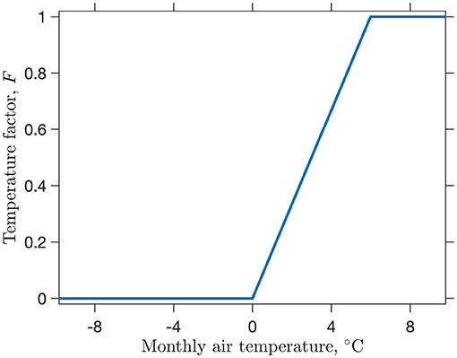
Figure 1. Monthly temperature factor for rainfall/snowfall partitioning or snowmelt estimation based on air temperature. Slope of the line between 0°C and 6°C is 0.167°C−1.
The factor, F, is also used to estimate monthly snowmelt following a degree-day or temperature-index approach. Here, F is multiplied by the sum of the snow water equivalent on the ground, PACK, for the previous month and the current month's snowfall, SNOW, to estimate snowmelt, MELT. The result is the amount of snow that will melt and be considered part of water input to the soil, W. Water input, W, to the soil storage is therefore the sum of rainfall and snowmelt. The snowpack at the end of month is then computed following Dingman (2015) as the proportion of precipitation that fell as snow and contributed to that month's snowpack, plus the previous month's snowpack that did not melt.
Potential evapotranspiration, PET, in this model is calculated using the Thornthwaite (1948) equation; however, other approaches that use air temperature (e.g., Hamon, 1961) could be used as well. The model assumes that if monthly water input exceeds monthly PET, then actual evapotranspiration, ET, takes place at the PET rate and the soil-water storage, S, increases or, if it is already at soil-water storage capacity (SC), it remains constant. The Thornthwaite (1948) equation for PET depends on monthly temperature and latitude, which is used to account for the varying number of days per month and hours of daylight (Criddle, 1958). When water input for a month is less than PET, ET is equal to the sum of water input and the amount of soil-water that can be removed from the soil storage for month i depending on the following exponential drainage function (Alley, 1984):
The app provides a table of monthly values (e.g., Table 1) and five graphs for any given location defined by a NOAA observing station location. The graphs display monthly water inputs to the soil-water storage that are divided into snowmelt and rainfall contributions, soil-water and snowpack storage, monthly temperature, and the snow and rain monthly fractions of precipitation. Table 1 is the monthly water balance output for Blacksburg, Virginia, at 37.2 °N latitude. The onset of snow inputs and snowpack occur in December and the snowpack reaches its peak in February, and melts in March. For the months when there is adequate supply of soil-water storage for the evaporative demand (October-May), ET is equal to PET. Recharge of the soil-storage begins in October and reaches its capacity the following month. The depletion of soil-water storage begins in June and continues into September as the evaporative demand is satisfied by removing water from the soil-water storage, S. The average monthly water surplus (W−ET−ΔS), i.e., water available for recharge and runoff, are the monthly inputs that are in excess of monthly ET and soil-water storage changes.
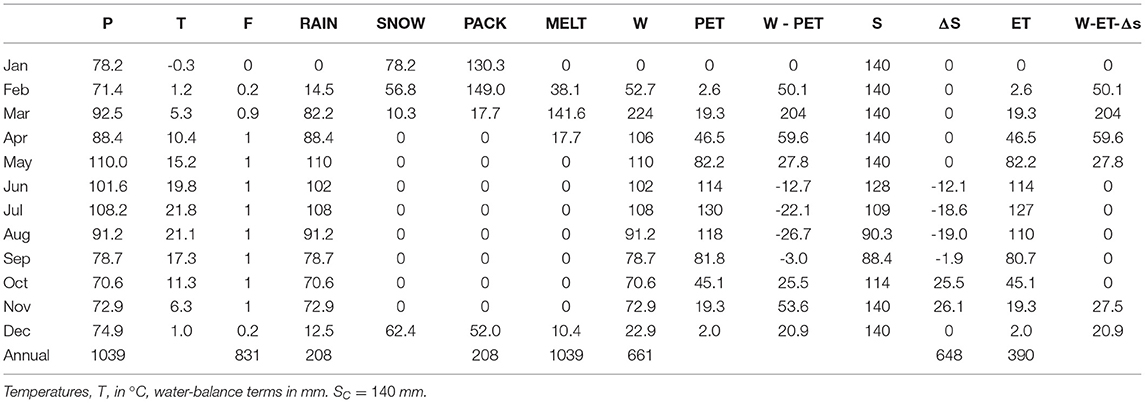
Table 1. Output of Thornthwaite-type monthly water balance for Blacksburg, VA.
Results: App Implementation and Features
The water balance app is a Shiny web application (https://shiny.rstudio.com/) and is hosted by CUAHSI. The web application can be run on any common internet browser on a computer, tablet, smartphone, or chromebook. Use of the app is free and does not require the user to download any special software. Source code for the app can be found at https://github.com/jpgannon/Water-Balance-App.
The app, shown in Figure 2 has six tabs which support a variety of functions. The landing page for the app is the “Output Plots” tab. Here students see five plots rendered from the results of the water balance function: soil inputs, soil storage, soil output, temperature, and precipitation. The plots will resize if the user changes the size of their browser window, and they can copy and paste the plots or save them by right-clicking on them. This facilitates saving the plots for activity write-ups. The plots will update automatically if the user makes changes to any of the settings on the left side of the app.
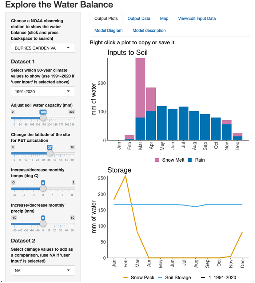
Figure 2. App interface showing two of the five plots, available inputs, and the tabs with additional functionality.
On the left panel, the user has several options. The first dropdown allows the user to select one of several thousand NOAA climate monitoring sites by either scrolling through the available options or typing to search. Next, the climate normal period can be switched between 1991–2020 and 1981–2010. The next slider down automatically starts at the soil water capacity of the site, which is the Available Water Storage measure for 100 cm of soil from the Natural Resource Conservation Service (NRCS) gNATSGO database (Soil Survey Staff, 2020). Moving this slider will change the water holding capacity in the model. The latitude slider similarly updates depending on the site chosen, and if moved, changes the latitude in the PET calculation in the model. The following two sliders, precipitation and temperature, always start at zero. If the user moves these sliders, they will add or subtract the value of the slider from each monthly value for the site chosen. For example if the temperature slider was moved to +1, it would add 1°C to the temperature data for each month at the site. Finally, if the user selects a climate normal period in the dropdown at the bottom of the column, those data will be added as a separate dataset to the plots. This can be used to compare the two climate normals, or if the user selects the same climate normal period for both, they can more clearly see how the water budget changes when they manipulate the sliders, as the second dataset is unaffected by user inputs.
The second tab at the top of the app is titled “output data” this tab shows all the output from the water balance model. This can be used to explore more quantitative differences between outputs, such as PET and AET. The data can also be downloaded using a download button at the bottom. This produces a comma-separated value (CSV) of the model output, which a user could then use to create their own visualizations, perhaps for an upper-level class or for custom figures for a lecture.
The third tab is the map tab. Here the user can zoom and pan around the contiguous US and see all available places for which they can calculate the water balance. If the user clicks a marker, that site will be selected in the left panel. If the user selects a site using the drop-down menu in the first tab, it will be highlighted on the map in the map tab.
The fourth tab allows the user to view or edit the input data for the model. When a site is chosen, its data populates this table. If the user double clicks on any value, they can enter a new value in its place, and the app will recalculate the water balance with the new data. This could be used to simulate a large flood or a drought, for instance. This tab has the additional functionality of allowing the user to put in a custom dataset from somewhere not included in the available data. If the user selects “User Input”, the first option in the dropdown menu for sites on the left panel, the view or edit input data becomes all zeros. The user can then enter their own temperature and precipitation values and use the sliders to change the available soil water capacity and latitude of the site.
Finally, the fourth and fifth tabs of the app offer a diagram of the model used, and a detailed description of the functionality of the app and the Thornthwaite soil water balance.
Discussion: Efficacy in a Classroom Environment
We used the app to introduce the water balance in two classes at Virginia Tech. One class was an introductory watershed hydrology class taught in the department of Forest Resources and Environmental Conservation and the other was an upper level undergraduate/introductory graduate level hydrology methods class taught in the Biological Systems Engineering department. The introductory class had around 60 students and the advanced class about 20. Both classes were taught in-person. After a short slideshow presentation introducing the water balance and a demonstration of the functionality of the app, students were provided with an activity. Both the lecture introduction and activity are included in the resources linked below. In both cases, these were individual activities in an in-person class. However, the application and included activities are likewise suitable for group-based activities and virtual or hybrid modalities, as no specific computing resources are required. After the activity, we asked the students to respond with how much they agreed with two statements to help determine if the students felt the app helped them understand the water balance, and if they enjoyed it more than previous activities using other methods, such as spreadsheets or hand calculations. The exact statements posed were:
“Compared to traditional approaches (spreadsheets, hand calculations, etc.), this exercise helped me learn hydrological concepts more effectively.”
“I found the online app helped enhance my learning.”
Students responded to each of the statements on a scale of 1–5 where 1 was “strongly disagree”, 3 was “agree”, and 5 was “strongly agree.” Figure 3 shows that students uniformly agreed that the app enhanced their learning and that the exercise helped them understand the material more effectively than a spreadsheet or hand calculation. For both courses, the most frequent response was “strongly agree” for both questions.
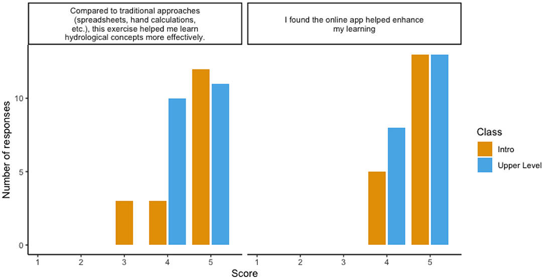
Figure 3. Responses to questions asked after water balance app activity. The x axis shows the score students marked for each question, where 1 was strongly disagree and 5 was strongly agree. The orange bars show responses of the students in the introductory level class and the blue bars show the responses of an upper level undergraduate/introductory graduate level class.
While the student response was positive, there are some drawbacks to using this web application as a sole replacement for other types of activities, depending on the learning goals for the class. For instance, exploring the app alone would not be appropriate if the topic is introduced in a class with the dual purpose of developing a conceptual understanding of the water balance and developing/practicing spreadsheet skills, graphing, unit conversion, or basic budget calculations. However, this app can also be used to facilitate these more advanced activities. For example, students could use the app to explore water balance concepts across the US and then export the data for a site of their choosing as a comma separated values (csv) file via the “output data” tab to perform further analysis by hand or in a spreadsheet program.
Ready-to-Use Activities
To facilitate use of this app in hydrology and earth science classrooms, we created three activities that can be used in a classroom after a short introduction to the water balance and the app. The questions addressed in these activities are as follows:
1. What controls how water is partitioned in a water balance?
2. What controls the amount of actual evapotranspiration at a site?
3. What is the difference between a water limited and energy limited system?
4. How can climate change affect the water balance?
The complete activities are available via CUAHSI's hydroshare, along with Powerpoint slides that introduce the water balance, a link to a video showing how to use the app, and a link to the app itself (https://www.hydroshare.org/resource/0ecadff374aa4a2b84e41f146d39f48c/).
Conclusions
The water balance is a crucial concept for students of hydrology to understand thoroughly, but is often confusing due to numerous interactions between parameters. Common methods used to explore the water balance can leave students bogged down in calculations or spreadsheet operations, taking away from their opportunity to become more comfortable with the core concepts. Interactive web-applications offer a solution, as they are a platform-agnostic and easy to use way for students to explore hydrologic concepts in the classroom.
Data Availability Statement
The original contributions presented in the study are included in the article/supplementary material, further inquiries can be directed to the corresponding author/s.
Author Contributions
Both authors listed have made a substantial, direct, and intellectual contribution to the work and approved it for publication.
Funding
The publication of this article was supported by the Virginia Tech Open Access Subvention Fund.
Conflict of Interest
The authors declare that the research was conducted in the absence of any commercial or financial relationships that could be construed as a potential conflict of interest.
Publisher's Note
All claims expressed in this article are solely those of the authors and do not necessarily represent those of their affiliated organizations, or those of the publisher, the editors and the reviewers. Any product that may be evaluated in this article, or claim that may be made by its manufacturer, is not guaranteed or endorsed by the publisher.
References
Alley, W. M. (1984). On the treatment of evapotranspiration, soil moisture accounting, and aquifer recharge in monthly water balance models. Water Resour. Res. 20, 1137–1149. doi: 10.1029/WR020i008p01137
Alley, W. M. (1985). Water balance models in one-month-ahead streamflow forecasting. Water Resour. Res. 21, 597–606. doi: 10.1029/WR021i004p00597
Arguez, A., Durre, I., Applequist, S., Vose, R. S., Squires, M. F., Yin, X., et al. (2012). Noaa's 1981-2010 U.S. climate normals: an overview. Bull. Am. Meteorol. Soc. 93, 1687–1697. doi: 10.1175/BAMS-D-11-00197.1
Azman, A. M., and Esteb, J. J. (2016). A coin-flipping analogy and web app for teaching spin-spin splitting in 1h nmr spectroscopy. J. Chem. Educ. 93, 1478–1482. doi: 10.1021/acs.jchemed.6b00133
Bedient, P., Huber, W., and Vieux, B. (2019). Hydrology and Floodplain Analysis. What's New in Engineering. Upper Saddle River, NJ: Pearson.
Black, P. E. (2007). Revisiting the Thornthwaite and Mather water balance. J. Am. Water Resour. Assoc. 43, 1604–1605. doi: 10.1111/j.1752-1688.2007.00132.x
Bransford, J. D., Brown, A. L., Cocking, R. R., et al. (2000). How People Learn: Brain, Mind, Experience and School. Vol. 11. Washington, DC: National Academy Press.
Criddle, W. D. (1958). Methods of computing consumptive use of water. J. Irrigat. Drainage Divis. 84, 1–27. doi: 10.1061/JRCEA4.0000048
Davie, T., and Quinn, N. W. (2019). Fundamentals of Hydrology. New York, NY: Routledge. doi: 10.4324/9780203798942
Dunne, T., and Leopold, L. B. (1978). Water in Environmental Planning. New York, NY: W.H. Freeman and Company.
Fitts, C. (2013). Groundwater Science. Scarborough, ME: Elsevier Science. doi: 10.1016/B978-0-12-384705-8.00001-7
Franklin, C., Kader, G., Mewborn, D., Moreno, J., Peck, R., Perry, M., et al. (2007). Guidelines for Assessment and Instruction in Statistics Education (GAISE) Report. Technical report, American Statistical Association.
Freeman, S., Eddy, S. L., McDonough, M., Smith, M. K., Okoroafor, N., Jordt, H., et al. (2014). Active learning increases student performance in science, engineering, and mathematics. Proc. Natl. Acad. Sci. U.S.A. 111, 8410–8415. doi: 10.1073/pnas.1319030111
Haak, D. C., HilleRisLambers, J., Pitre, E., and Freeman, S. (2011). Increased structure and active learning reduce the achievement gap in introductory biology. Science. 332, 1213–1216. doi: 10.1126/science.1204820
Hagtvedt, R., Jones, G. T., and Jones, K. (2007). Pedagogical simulation of sampling distributions and the central limit theorem. Teach. Stat. 29, 94–97. doi: 10.1111/j.1467-9639.2007.00270.x
Hamon, W. R. (1961). Estimating potential evapotranspiration. J. Hydraul. Divis. 87, 107–120. doi: 10.1061/JYCEAJ.0000599
Hiscock, K. M., and Bense, V. F. (2021). Hydrogeology: Principles and Practice. Hoboken, NJ: John Wiley & Sons.
Hornberger, G. M., Wiberg, P. L., Raffensperger, J. P., and D'Odorico, P. (2014). Elements of Physical Hydrology. Baltimore, MD: JHU Press.
McCabe, G. J., and Markstrom, S. L. (2007). A Monthly Water-Balance Model Driven by a Graphical User Interface. Open-File report 2007-1088, US Geological Survey, Reston, VA. doi: 10.3133/ofr20071088
McCabe, G. J., and Wolock, D. M. (2011). Independent effects of temperature and precipitation on modeled runoff in the conterminous united states. Water Resour. Res. 47, W11522. doi: 10.1029/2011WR010630
Soil Survey Staff (2020). Gridded National Soil Survey Geographic (gNATSGO) Database for the Conterminous United States. United States Department of Agriculture, Natural Resources Conservation Service.
Steenhuis, T., and Van der Molen, W. (1986). The Thornthwaite-Mather procedure as a simple engineering method to predict recharge. J. Hydrol. 84, 221–229. doi: 10.1016/0022-1694(86)90124-1
Taylor, J. C., van de Giesen, N., and Steenhuis, T. S. (2006). West Africa: volta discharge data quality assessment and use. J. Am. Water Resour. Assoc. 42, 1113–1126. doi: 10.1111/j.1752-1688.2006.tb04517.x
Thornthwaite, C. W. (1948). An approach toward a rational classification of climate. Geograph. Rev. 38, 55–94. doi: 10.2307/210739
Thornthwaite, C. W., and Mather, J. R. (1957). Instructions and tables for computing potential evapotranspiration and the water balance. Publ. Climatol. 10:311.
Tillman, F. D., Gangopadhyay, S., and Pruitt, T. (2017). Understanding the past to interpret the future: comparison of simulated groundwater recharge in the Upper Colorado river basin (USA) using observed and general-circulation-model historical climate data. Hydrogeol. J. 25, 347–358. doi: 10.1007/s10040-016-1481-0
Westenbroek, S. M., Kelson, V., Dripps, W., Hunt, R., and Bradbury, K. (2010). SWB-A Modified Thornthwaite-Mather Soil-Water-Balance Code for Estimating Groundwater Recharge. Techniques and Methods 6-A31, US Geological Survey. doi: 10.3133/tm6A31
Keywords: water balance, water budget, web app, teaching, hydrology
Citation: Gannon JP and McGuire KJ (2022) An Interactive Web Application Helps Students Explore Water Balance Concepts. Front. Educ. 7:873196. doi: 10.3389/feduc.2022.873196
Received: 10 February 2022; Accepted: 11 March 2022;
Published: 12 April 2022.
Edited by:
Anne Jefferson, Kent State University, United StatesReviewed by:
Arial Shogren, University of Alabama, United StatesMason Stahl, Union College, United States
Copyright © 2022 Gannon and McGuire. This is an open-access article distributed under the terms of the Creative Commons Attribution License (CC BY). The use, distribution or reproduction in other forums is permitted, provided the original author(s) and the copyright owner(s) are credited and that the original publication in this journal is cited, in accordance with accepted academic practice. No use, distribution or reproduction is permitted which does not comply with these terms.
*Correspondence: John P. Gannon, anBnYW5ub25AdnQuZWR1