Comparative Judgement for Linking Two Existing Scales

This article describes an efficient way of using comparative judgement to calibrate scores from different educational assessments against one another (a task often referred to as test linking or equating). The context is distinct from other applications of comparative judgement as there is no need to create a new achievement scale using a Bradley-Terry model (or similar). The proposed method takes advantage of this fact to include evidence from the largest possible number of examples of students’ performances on the separate assessments whilst keeping the amount of time required from expert judges as low as possible. The paper describes the method and shows, via simulation, how it achieves greater accuracy than alternative approaches to the use of comparative judgement for test equating or linking.

Introduction

Test equating and linking refers to methods that allow us to identify the scores on one assessment that are equivalent to individual scores on another. This paper concerns the use of comparative judgement (CJ) for linking tests. This context for the use of CJ differs from others in that all the representations included in the CJ study (that is, the exam scripts) already have scores assigned from traditional marking. Therefore, there is no need to use CJ to re-score them. Rather, the aim is simply to calibrate the existing scores from separate assessments onto a common scale. Only enough representations to facilitate calibration need to be included in the associated CJ study. This paper will describe how CJ has been used for test linking in the past, and, more importantly, show how we can improve on existing approaches to increase efficiency.

The idea of using CJ for test linking and equating has existed for a long time. The usual motivation for research in this area is the desire to calibrate assessments from different years against one another. Specifically, to identify grade boundaries on 1 year’s test that represent an equivalent level of performance to the grade boundaries that were set on the equivalent test the previous year. A method by which CJ can be used for this task was formalized by Bramley (2005). The method works broadly as described below.

Suppose we have two test versions (version 1 and version 2) and, for each score on version 1, we wish to find an equivalent score on version 2. That is, the score that represents an equivalent level of performance. To begin with, we select a range of representations from each test version. By “representations,” for this type of study, we usually mean complete scanned copies of students’ responses to an exam paper (“scripts” in the terminology used in British assessment literature). Typically, around 50 representations are selected from each version covering the majority of the score range. Next, the representations are arranged into sets that will be ranked from best to worst by expert judges. In this article, we refer to these sets of representations that will be ranked as “comparison sets” (or just “sets”). In Bramley (2005) and elsewhere these sets of scripts are referred to as “packs.” Each comparison set contains representations from both test versions. In a pairwise comparison study, each set would consist of just two representations—one from each test version. For efficiency (particularly in paper-based studies) representations might be arranged into sets of up to 10 each with five representations from version 1 and five from version 2. This process is repeated multiple times (in a paper-based study this involves making multiple physical copies of scripts) so that representations are included in several sets and the precise combination of representations in any set is, as far as possible, never repeated.

When we fit a Bradley-Terry model we are attempting to place all of the representations in the model on a single scale. This process will only work if we have some way of linking every pair of objects in the model to one another by a series of comparisons. For example, representation A may never have been compared to representation B directly. However, if both representation A and representation B have been compared to representations C, D, E and F, then we should be able to infer something about the comparison between representations A and B. The technical term for this requirement is that all objects are connected. If our aim is to fit a Bradley-Terry model, then ensuring that all objects are connected to one another is an important part of the design—by which we mean the way in which different representations are assigned to sets (possibly pairs) that will directly compared by judges. Two representations are directly connected if they are ever in the same comparison set. Alternatively, two representations may be indirectly connected if we can find a sequence of direct connections linking one to the other. For example, representations A and D would be indirectly connected if representation A was included in a comparison set with representation B, representation B in a (different) comparison set with representation C, and representation C in (yet another) comparison set with representation D. A design is connected if all possible pairs of representations are connected either directly or indirectly.

Having allocated representations to comparison sets, each set is assigned to one of a panel of expert judges who ranks all of the representations in the set based on their judgements of the relative quality of the performances. In the case of pairwise comparison, where each set consists of only two representations, this simply amounts to the judge choosing which of the two representations they feel demonstrates superior performance.

Once all the representations in each set have been ranked, these rankings are analyzed using a statistical model. For ranking data, the correct approach is to use the Plackett-Luce model (Plackett, 1975), which is equivalent to the rank ordered logit model or exploded logit model described in Allison and Christakis (1994). In the case of pairwise comparisons, analysis is completed using the equivalent, but simpler, Bradley-Terry model (Bradley and Terry, 1952). Whichever model is used, the resulting analysis produces a measure of the holistic quality of each representation depending upon which representations it was deemed superior to, which it was deemed inferior to, and the number of such judgements. These measures of holistic quality (henceforth just “measures”) are on a logit scale. This means that, by the definition of the Bradley-Terry model, if representations A and B have estimated CJ measures of ${\theta }_A$ and ${\theta }_B$, then the probability that a randomly selected judge will deem representation A to display superior performance to representation B $\left(P_{AB}\right)$ is given by the equation:

$P_{AB}=\frac{\exp \left({\theta }_A-{\theta }_B\right)}{1+\exp \left({\theta }_A-{\theta }_B\right)}$

Having fitted a Bradley-Terry model, the performances of all representations are now quantified on a single scale across both test versions. That is, although the test versions are different and the raw scores cannot be assumed to be equivalent, the process of comparative judgement has yielded a single calibrated scale of measures that works across both tests. This can now be used to calibrate the original score scales against one another. The purpose of the final calibration step is that, once it is completed, we can make some inferences about the relative performances of all students that took either of the test versions—not just the sample of students included in the CJ study.

The usual way calibration is completed is illustrated in Figure 1. Regression analysis is used to estimate the relationship between scores and measures within each test. Then, the vertical gap between these estimated lines is used to identify the scores on version 2 of the test equivalent to each score on version 1.

FIGURE 1

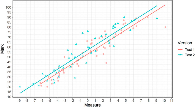
FIGURE 1. Illustrating the method of linking using CJ suggested by Bramley (2005).

Traditionally, the regression lines are not defined to be parallel. However, in most published studies, the differences in the slopes of the two lines are self-evidently small and, on further inspection, usually not statistically significantly different. As a result, in most cases it would make sense to identify a single adjustment figure. That is, how many score points easier or harder is version 2 than version 1? The regression method for this approach would be to identify the most accurate linear predictions of the raw original scores of each representation (denoted $x_i$ for the ith representation) of the form:

${\widehat{x}}_i={\beta }_0+{\beta }_1{\theta }_i+{\beta }_2{v}_i$

Where ${\widehat{x}}_i$ is the predicted raw score of the ith representation, ${\theta }_i$ is the CJ measure of the representation, and $v_i$ is a version indicator equal to 1 if the ith representation is from version 2 and equal to 0 otherwise. The coefficients of the regression model are ${\beta }_0$, ${\beta }_1$, and ${\beta }_2$. In this formulation, our particular interest is in the coefficient ${\beta }_2$ which gives a direct estimate of how much easier version 2 is compared to version 1.

The method suggested by Bramley (2005) has been trialed numerous times (e.g., Black and Bramley, 2008; Curcin et al., 2019) and, in general, these trials have produced plausible results regarding the relative difficulty of different test versions.

The regression method above might be labelled score-on-measure as the traditional test scores are the dependent variables and the CJ measures of the quality of each representation are the predictors. However, as described by Bramley and Gill (2010), the regression need not be done this way around. That is, we could perform (measure-on-score) regression with the CJ measures as the dependent variable and the scores as the predictors. Specifically, the regression formula would be:

${\widehat{\theta }}_i={\gamma }_0+{\gamma }_1{x}_i+{\gamma }_2{v}_i$

Where ${\widehat{\theta }}_i$ is the predicted CJ measure of the ith representation and ${\gamma }_0$, ${\gamma }_1$, and ${\gamma }_2$ are the regression parameters of this alternative formulation. The relative difficulty of version 2 relative to version 1 is then estimated by $\left(\frac{-{\gamma }_2}{{\gamma }_1}\right)$. In other words, this estimates how much higher a score on version 2 needs to be to predict the same fitted measure as would be predicted by a given score on version 1.

In many practical examples, the differences between the two methods are small (see an investigation by Bramley and Gill, 2010, for one such example). However, during the current research it became clear that large differences between the two methods can occur under certain circumstances. The reasons for this will be explored later in the report. For now, it is sufficient to note that, if the derived CJ measures are reliable and are highly correlated with the original scores then the difference between the two regression approaches should be small. However, knowing that different approaches are possible will be helpful for explaining the results of the simulations later in the report. Other methods of analyzing the same kind of data are also possible (for example, the “standardized major axis,” see Bramley and Gill, 2010). However, the two methods mentioned above, along with the new method to be introduced next, are sufficient for the purposes of this paper.

The focus of this paper is to show how a slightly different methodological approach can make the use of CJ for test linking more accurate. In particular, as can be seen from the above description, current approaches to the use of CJ to link existing score scales tend to rely on relatively small samples of representations (around 50) from each test version. Relying on small samples of representations is undesirable as it may lead to high standard errors in the estimates. Since each representation needs to be judged many times by expert judges, under existing approaches, the number of representations included in the study cannot be increased without incurring a significant additional cost. The goal of the newly proposed approach is to allow us to include a greater number of representations in a CJ study to link two existing scales without increasing the amount of time and resource needed from expert judges.

Note that the proposed approach is limited to CJ studies where out goal is to calibrate two existing score scales against one another. As such, the key change in the revised methodology is that it bypasses the need for the Bradley-Terry model in the process. That is, in the newly proposed approach there is no need to conduct a full CJ assessment and produce estimated measures for each representation in the study.

The newly suggested method works as follows. Representations are arranged into pairs of one representation from version 1 of the test and one representation from version 2 of the test. For each pair of representations, an expert judge decides which of the two representations is superior. Next, the difference in scores between the two representations is plotted against whether the representation from version 2 of the test was judged to be superior. An example of such a chart is given in Figure 2. The x-axis of this chart denotes the difference in scores. Each judgement is represented by a dot that is close to 1.0 on the y-axis if the version 2 representation is judged superior and is close to 0.0 if it is judged to be inferior (a little jitter has been added to the points to allow them to be seen more easily). As can be seen, in this illustration, where the score awarded to version 2 greatly exceeds the score awarded to version 1, the version 2 representation is nearly always deemed superior. Where the score on version 2 is lower than that on version 1, the version 2 representation is less likely to be judged superior.

FIGURE 2

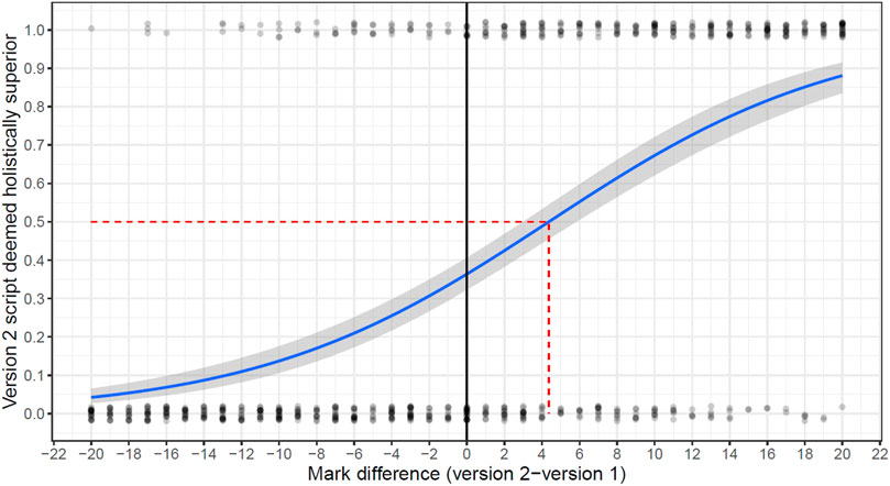
FIGURE 2. Illustrating the newly proposed method of linking using CJ.

The relationship between the score difference and the probability that the version 2 representation is deemed superior is modelled statistically using logistic regression. This is illustrated by the solid blue line in Figure 2. To determine how much easier (or harder) version 2 is compared to version 1, the aim is to identify the point at which this line crosses 0.5; that is, where the version 2 representation is as likely to be judged superior as it is to be judged inferior. In the case of Figure 2, the data would indicate that version 2 appears to be roughly 4 score points easier than version 1.

We denote the outcome of the ith paired comparison as $y_i$ with a value equal to 1 if the judge deems the representation from test version 2 as superior and equal to zero if the representation from test version 1 is deemed superior. We denote the original score of the representation from test version 2 within the ith paired comparison as $x_{2i}$ and the score of the representation from test version 1 as $x_{1i}$. The equation for the logistic regression model is as follows.

$P\left(y_i=1\right)=\frac{\exp \left({\delta }_0+{\delta }_1\left(x_{2i}-x_{1i}\right)\right)}{1+\exp \left({\delta }_0+{\delta }_1\left(x_{2i}-x_{1i}\right)\right)}$

The $\delta$ coefficients in this equation are just the usual logistic regression parameters. The number of score points by which version 2 is easier than version 1 is estimated by $\left(\frac{-{\delta }_0}{{\delta }_1}\right)$.

The newly proposed method, and the avoidance of using a Bradley-Terry model in particular¹, has several advantages:

• There is no need for the same representations to be judged many times. If we were intending to create a reliable set of CJ measures, then it would be necessary for every representation to be judged multiple times. According Verhavert et al. (2019), each representation should be included within between 10 and 14 paired comparisons in order to for CJ measures to have a reliability of at least 0.7. In contrast, the new procedure described above will work even if each representation is only included in a single paired comparison.

• Similarly, because we are not intending to estimate CJ measures for all representations using a Bradley-Terry model, there is no need for the data collection design to be connected.

• As a consequence of the above two advantages, we can include far more representations within data collection without requiring any more time from expert judges. Including a greater number of representations should reduce sampling errors leading to improved accuracy. Whilst in the past, exam scripts were stored physically, they are now usually stored electronically as scanned images. As such, accessing script images is straightforward meaning that the inclusion of greater numbers of representations in a CJ study need not incur any significant additional cost.

Note that, all of the formulae for the new approach can be applied regardless of whether the data collection design collects multiple judgements for each representation, or whether each representation is only included in a single pair. However, we would not expect applying the formulae from the new approach to data that was collected with the intention of fitting a Bradley-Terry model to make estimates any more accurate. The potential for improved accuracy only comes from the fact that the new approach allows us to incorporate greater numbers of representations in a study (at virtually no cost).

We call our new approach to the use of CJ for test linking “simplified pairs.” This approach has been described and demonstrated previously in Benton et al. (2020). This current paper will show via simulation, why we expect “simplified pairs” to provide greater accuracy than previously suggested approaches.

Methods

A simulation study was used to investigate the potential accuracy of the different approaches to using comparative judgement for linking tests. The parameters for the simulation, such as the specified standard deviation of true CJ measures of the representations and how these are associated with scores, were chosen to give a good match to previous real empirical studies of the use of CJ in awarding. Evidence that this was achieved will be shown as part of the results section.

The process for the simulation study was as follows:

1. Simulate true CJ measures for 20,000 representations from each of test version 1 and test version 2. We denote the true CJ measure of the ith representation from test version 1 as ${\theta }_i$ and the true CJ measure of the jth representation from test version 2 as ${\theta }_j$. In both cases these are simulated to follow a normal distribution with a mean of 0 and a standard deviation of 2.

2. Simulate raw scores for the 20,000 representations from each test version. We denote the score of the ith representation from test version 1 as $x_i$ and the score of the jth representation from test version 2 as $x_j$. The scores were initially simulated from normal distributions according to

$x_i=50+8{\theta }_i+6{\epsilon }_i$

$x_j=54+8{\theta }_j+6{\epsilon }_j$

Where ${\epsilon }_i$ and ${\epsilon }_j$ were simulated from standard normal distributions with a mean of 0 and a standard deviation of 1. These initially simulated scores were rounded to whole numbers and truncated to be between 0 and 100. The resulting simulated scores had means of 50 and 54 for test version 1 and test version 2 respectively. For both test versions, the standard deviation of the resulting scores was approximately 17.

3. Sample 50 representations from version 1 and 50 representations from version 2. Within each test version, sampling was done so that the scores of selected representations were evenly spaced out between 20 and 90.²

4. Create the design of a pairwise CJ study that might provide the data for fitting a Bradley-Terry model. This design should ensure that:

a. Every pair compares a representation from test version 1 to a representation from test version 2.

b. Each representation is included in $N_{CR}$ pairs (where $N_{CR}$ is a key variable for the study between 2 and 30).

c. Only representations whose raw scores differ by 20 or less should be paired.

d. As far as possible, exact pairs of representations are never repeated.

We define T as the total number of pairs in the study. Since we have sample 50 representations from each test version $T=50\ast N_{CR}$.

5. Simulate the results of the paired comparisons defined in step 4. We imagine that an expert judge has to determine which of the two representations in each pair is superior. The probability that the jth representation from version 2 is deemed to display superior performance to the ith representation from version 1 is given by the formula:

$P_{ji}=\frac{\exp \left({\theta }_j-{\theta }_i\right)}{1+\exp \left({\theta }_j-{\theta }_i\right)}$

6. Now use the results of this simulated paired comparison study to estimate the difference in difficulty between the two test versions using each of the three methods described earlier. Specifically:

a. Fit a Bradley-Terry model to the data to generate measures and use a regression of scores on measures.

b. Based on the CJ estimates from the same Bradley-Terry model, use a regression of measures on scores.

c. Directly estimate the difference in difficulty between test versions using the logistic regression method described earlier. This represents using the analysis methodology from our newly suggested approach but without taking advantage of the potential improvements to the data collection design.

7. Now, using the same set of 20,000 representations from each version (from steps 1 and 2), simulate a full simplified pairs study. The aim is that the study will include the same number of pairs as the other methods (i.e., T), but that we will sample more representations and only include each of them in a single pair. To begin with, we sample T representations from version 1 and T representations from version 2. Within each test version, representations were again selected so that their scores were evenly spaced out between 20 and 90.

8. Using these freshly selected representations, create the design of a simplified pairs study (i.e., assign representations to pairs). This design should ensure that:

a. Every pair compares a representation from test version 1 to a representation from test version 2.

b. Each representation is included in exactly 1 pair.

c. Only representations whose raw scores differ by 20 or less should be paired.

Since each representation is included in a single pair this will result in T pairs.

9. Simulate the results of these fresh paired comparisons using the same formula as in step 5.

10. Using the data from these fresh paired comparisons, apply logistic regression to generate an estimate of the relative difficulty of version 1 and version 2. This is the simplified pairs estimate of the difference in the difficulty of the two tests.

11. Repeat the entire process (steps 1–10) 2,000 times.

All analysis was done using R version 4.0.0 and the Bradley-Terry models were fitted using the R package sirt (Robitzsch, 2019).

The above procedure was repeated with the total number of pairs in each study (T) taking each of the values 100, 200, 300, 400, 500, 750, 1000, and 1500. For every method other than the full simplified pairs approach, where each representation is only included in a single paired comparison, these values correspond to the number of paired comparisons for each of the 50 representations for each test version $\left(N_{CR}\right)$ being 2, 4, 6, 8, 10, 15, 20, and 30.

Note that the first 2 steps of the simulation process produce realistic means and standard deviations of the simulated scores. That is, the means (50 and 54 for the two respective test versions) and the standard deviations (approximately 17 for each test version) are typical of the values we tend to find in real tests of this length.

As can be seen from the above description, test version 2 is simulated to be exactly 4 score points easier than version 1. This size of difference in difficulty was chosen as it reflects the typical absolute amount (as the percentage of maximum available score) by which GCSE component grade boundaries changed between 2015 and 2016³. As such, it is typical of the kind of difference we’d need our methods to handle in practice.

As mentioned above, the way in which representations were sampled to be evenly spread across the score range from 20 to 90 per cent (steps 3 and 7) reflects the way previous CJ studies for linking tests have been done in practice. Representations with very high scores are usually excluded as, if two candidates have answered nearly perfectly, it can be extremely difficult to choose between them. Representations with scores below 20 per cent of the maximum available are also typically excluded as, in practice, they often have many omitted responses meaning that judges would have very little evidence to base their decisions on.

Further evidence of how the simulation design produces results that are representative of real studies of this type will be provided later.

The aim of analysis was to explore the accuracy with which each of the different methods correctly identified the true difference in difficulty between the two test versions (4 score points). This was explored both in terms of the bias of each method (i.e., the mean estimated difference across simulations compared to the true difference of 4), and the stability of estimated differences across simulations.

In addition to recording the estimated differences in difficulty using each method within each simulation, we also recorded the standard errors of the estimates that would be calculated for each method. This helps to understand how accurately each method would allow users to evaluate the precision of their estimates. Specifically:

• For the score-on-measure regression approach the standard error of the estimated difference in difficulty is simply given by the standard error of ${\beta }_2$ in the regression. Note that the use of this standard error requires that the assumptions underpinning the regression itself are correct. However, the usual assumption that the observations in the regression are independent (e.g., in Figure 1) is, in fact, incorrect. Since all CJ measures were estimated simultaneously, the CJ measures of different representations are, in fact, correlated with larger (positive) correlations between representations that were directly compared. Despite this concern, these kind of estimates of uncertainty have been used in previous research (e.g., Curcin et al., 2019) and it was of interest to examine their accuracy.

• For the measures on scores approach the standard error of any estimate is derived using the delta method. Specifically, if we label the parameter covariance matrix from the regression model as $C\left(\mathit{\gamma }\right)$, then the standard error of the estimated difference in difficulty is given by:

$StandardError=\sqrt{G^{T}C\left(\mathit{\gamma }\right)G},\mathrm{where}G=\left(\begin{array}{c}0\\ \left(\frac{{\gamma }_2}{{\gamma }_1^2}\right)\\ \left(\frac{-1}{{\gamma }_1}\right)\end{array}\right)$

Once again, these standard errors rely on the assumptions of the regression being correct and, as such, may suffer from the same issues as those based on scores on measures regression.

• For the simplified pairs method, we can also use the delta method to create standard errors. Specifically, if we denote the parameter covariance matrix from the logistic regression as $V\left(\mathit{\delta }\right)$ then the standard error of the estimated difference in difficulty is given by:

$StandardError=\sqrt{H^{T}V\left(\mathit{\delta }\right)H},\mathrm{Where}H=\left(\begin{array}{c}\left(\frac{-1}{{\delta }_1}\right)\\ \left(\frac{{\delta }_0}{{\delta }_1^2}\right)\end{array}\right)$

These standard errors rely on the assumptions underpinning the logistic regression being correct. Within our simulation these assumptions are plausible for the full simplified pairs approach. In particular, if each representation is only used once, observations in the logistic regression are independent. For the use of the logistic regression approach based on the simulated data where the same representations are used multiple times the assumption of the independence of observations is quite clearly incorrect and so these standard errors were not retained⁴.

To help verify the realistic nature of the simulation study, for all methods using a Bradley-Terry model, the reliability of the CJ measures was recorded within each simulation. This was calculated both in terms of an estimated scale separation reliability (SSR, see Bramley, 2015) and also in terms of the true reliability calculated as the squared correlation between estimated CJ measures and the true simulated values. Correlations between estimated CJ measures and raw scores on each test version were also calculated and recorded from each simulation.

Results

A Digression on the Realistic Nature of the Simulation

To begin with it is worth noting that, by design, the simulation produced results regarding the reliability of CJ measures that were very consistent with those typically seen in empirical studies. For example, for the simulations involving 750 comparisons in total and 15 per representation (a typical number of comparisons per representation in previous studies of this type), across simulations, the median SSR was 0.93 (the median true reliability⁵ was also 0.93), and the median correlation between CJ measures and raw scores was 0.92 (for both test versions). These values match the median reliabilities and correlations between raw scores and estimated CJ measures across 10 real studies based on using pairwise comparative judgement to link score scales published by Curcin et al. (2019, page 41, Table 7).

The average level of reliability from 15 comparisons per representation (0.93), which matches the average values from real empirical studies of this type (Curcin et al., 2019), is somewhat higher than research on the use of CJ in other contexts suggests is typical (for example, see Verhavert et al., 2019). Although this is not the main focus of the article, we will briefly digress to explain why the discrepancy occurs. In short, we believe it is largely because, in studies concerned with linking two existing scales, all representations have already been scored in a non-CJ way to begin with. The analysis can capitalize on this additional data from the original scores in ways that are not possible if CJ if the sole method by which representations are being assessed. Of course, there is a cost to scoring all representations before beginning a CJ study, so this should not be taken as a recommendation that this should be done in general.

Part of the reason for the higher reliability coefficients in empirical CJ studies concerned with linking existing scales (e.g., Curcin et al., 2019) is the way in which representations are selected. Unlike the studies by Verhavert et al. (2019), only a sample of the possible representations are included in the CJ study and this sample is not selected at random. Rather, representations are deliberately selected with scores that are evenly spread across the available range between 20 and 90 per cent of the paper total. This ensures that a wider range of performances is included in each study than would be the case by selecting representations purely at random. We would expect this to mean that the standard deviation of the true CJ measures included in such a study is higher than in the population in general and, as a result, reliability coefficients are expected to be higher.

In addition, because, by design, representations are only compared to those with relatively similar scores, some of the advantages usually associated with adaptive comparative judgement (ACJ, see Pollitt, 2012) are built into the method. This allows higher reliabilities to be achieved with smaller numbers of comparisons. Note that, although the method has some of the advantages of ACJ, it is not actually adaptive. Which representations are compared to one another is not amended adaptively dependent upon the results of previous comparisons. As such, concerns about the inflation of reliability coefficients in an adaptive setting (Bramley and Vitello, 2019) do not apply.

Understanding the reasons for these high reliability coefficients, and that these reflect the values that we see on average in real empirical studies of this type is important as it allows us to have confidence in the remainder of the results presented in this paper.

Before returning to the main subject of this paper we note that, as expected, within our own simulation study, the reliability of the CJ measures increased with the number of comparisons per representation. The median reliability was just 0.2 if only 2 comparisons per representation were used, rose to above 0.7 for 4 comparisons per representation, and was 0.96 for 30 comparisons per representation⁶.

Biases and Standard Errors of Different Methods

Our main interest is in the bias and variance (i.e., stability) of the various methods for estimating the relative difficulty of two tests. Figure 3 shows the results of the analysis in terms of the mean estimated difference in the difficulty of the two tests from each method. The mean estimated difference from each method is compared to the known true difference (4 score points) represented by the thick grey line. The mean difference between the estimated and actual differences in test difficulty provides an estimate of bias and this is shown by the secondary y-axis on the right-hand side. Note that the method labelled “direct logistic method” (the purple dashed line) relates to results from applying the newly proposed analysis methodology but with the same data as other methods. In contrast the method labelled “simplified pairs” relates to using our method from a data collection design with each representation being included in just 1 comparison. As long as the total number of pairs in the study is at least 200, 3 of the methods have levels of bias very close to zero. The two approaches based on logistic regression are essentially unbiased across all sample sizes. However, the most interesting result from Figure 3 is the evident bias of using the Bradley-Terry model in combination with a regression of scores on measures—that is, the dominant method of using comparative judgement in standard maintaining in studies of this type to date.

FIGURE 3

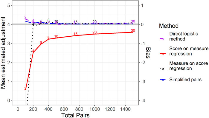
FIGURE 3. Mean estimated difference in difficulty between test versions across simulations for different methods by total number of pairs per study. Note that the true level of difference in difficulty is 4 (the solid grey line). For the three methods in which representations were included in multiple pairs, the number of pairs per representation is noted just above the relevant line.

The score-on-measure regression method has a negative bias. That is, on average it underestimates the scale of the difference in difficulty between the two test versions. The reason for this is to do with the way in which representations are selected for most studies of this type. To understand why this is, imagine a situation where, perhaps due to having a very small number of comparisons per representation, the CJ measure was utterly unreliable and had zero correlation with the scores awarded to representations. In this instance, the score-on-measure regression (e.g., Figure 1) would yield two horizontal lines. The vertical distance between these lines would actually be pre-determined by the difference in the mean scores of the representations we had selected from each version. In our study, since we have deliberately selected the same range of scores for each test version, this difference is equal to zero.

As the number of comparisons per representation increases, the size of the bias reduces but does not immediately disappear. With low, but non-zero, correlations between scores and measures the estimated difference between test versions will hardly be adjusted from the (predetermined) mean difference between the selected representations. As such, the bias in the method would persist. As the number of comparisons per representation increases, this bias becomes much smaller. However, due to the fact that, in this simulation, even the true CJ measures are not perfectly correlated with scores (correlation of 0.95) this bias never completely disappears.

Aside from bias, we are also interested in the stability of estimates from different methods—that is, their standard errors. According to the Cambridge Dictionary of Statistics (Everitt and Skrondal, 2010) a standard error (SE) is “the standard deviation of the sampling distribution of a statistic” (page 409). In our case, the “statistic” we are interested in is the estimated difference in the difficulty of two tests by some method and the “sampling distribution” is observable from the simulations we have run. As such, we can calculate the true standard error of each method by calculating the standard deviation of estimated differences in difficulty across simulations. Figure 4 shows how the standard errors of the estimates of differences in difficulty change depending upon the total number of pairs in the study. Somewhat counterintuitively, Figure 4 shows that the score-on-measure approach becomes less stable (i.e., has higher standard errors) as the number of comparisons per representation increases. In other words, increasing the amount of data we collect makes the results from this method more variable. This result is due to the fact that, as described above, where the correlation between original raw scores and measures is low, the method will hardly adjust the estimated difference in the difficulty of test versions from the predetermined mean score difference of zero. As such, across multiple replications of the simulations with low numbers of comparisons per representation, the score-on-measure method will reliably give an (incorrect) estimate close to zero. As the number of comparisons per representation increases, and the correlation between scores and measures becomes stronger, so the method will actually begin making substantive adjustments to account for differences in the holistic quality of responses and so the results become more variable across simulations.

FIGURE 4

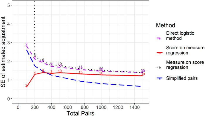
FIGURE 4. Standard deviation of estimated difference in difficulty between test versions across simulations for different methods by total number of pairs per study. For the three methods in which representations were included in multiple pairs, the number of pairs per representation is noted just above the relevant line.

Figure 4 shows that if we only allow 2 comparisons per script then the measure-on-score regression approach is extremely unstable. However, for larger numbers of comparisons per script, the standard errors of the measure-on-score and the direct logistic methods using the same set of data are very similar. This is, perhaps, unsurprising as, in essence, both methods are doing the same thing, although the score-on-measure regression uses one more step in the calculation. That is, both methods attempt to find the score difference where representations from either test version are equally likely to be deemed superior by a judge.

Of most interest are the simplified pairs results based on using the same total number of paired comparisons but only using each representation once. For any given number of total pairs, this approach is more stable than either of the two alternative unbiased methods (measure-on-score regression or direct logistic). Furthermore, the simplified pairs approach yields roughly the same standard errors with 300 comparisons in total as can be achieved with five times as many comparisons (30 per representation or 1500 in total) for either of the other two approaches. This suggests that avoiding the use of the Bradley-Terry model, including as many different representations as possible in the exercise, and using logistic regression to estimate the difference in the difficulty of two test versions can lead to huge improvements in efficiency in terms of the amount of time required from expert judges. This also suggests that including 300 comparisons in a simplified pairs study should provide an acceptable level of reliability.

Figure 4 concerns the true standard errors of each method – that is, the actual standard deviations of estimates across simulations. However, true standard errors are not generally observable outside of simulation studies and we need an alternative way of estimating standard errors in practice. How this might be done within each approach was described earlier and some formulae were provided. Figure 5 compares the median estimated standard errors of each method, based on the formulae provided earlier, to actual standard errors within each size of study. As can be seen, estimated standard errors for both score-on-measure and measure-on-score regression tend to be too high. The reasons for this as regards score-on-measure regression have largely already been discussed. For measure-on-score regression the issue relates to the assumptions of the regression model.

FIGURE 5

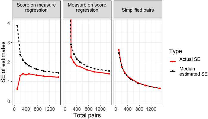
FIGURE 5. Plot of median estimated standard errors of each method and actual standard deviations of estimated difference in difficulty for different total study sizes.

The estimated standard errors come from the regression of CJ measures on scores using data of the type shown in Figure 1. Estimating standard errors essentially involves asking how much we’d expect the gap between two regression lines to change if we were to rerun the study with a fresh sample of representations. In some studies, though not here, this is estimated using bootstrapping (e.g., Curcin et al., 2019) which involves literally resampling from the points in charts like Figure 1 (with replacement) many times and measuring the amount by which the gap between lines varies.

The fact that the assumption of independent errors does not hold, explains the discrepancy between the actual and estimated standard errors of measure-on-score regression. Specifically, because every comparison is between a version 1 representation and a version 2 representation, the gap between regression lines will be less variable across samples than would be expected by imagining every point in the regression as being independent. In short, ensuring that every comparison in a pairwise design is between versions is a good thing because it reduces the instability of the gap between regression lines. However, it is a bad thing for accurately estimating standard errors as it leads to a violation of the regression assumptions.

In the simulations described here, estimated confidence intervals based purely on the regression chart tend to be wider than necessary. In other situations, we would expect the error in estimation to work the other way. For example, imagine that the design of a CJ study included large numbers of comparisons within test versions but only a handful of comparisons between version 1 and version 2. Instinctively, we can tell that such a design would provide a very poor idea of the relative difficulty of the two test versions. However, with sufficient comparisons within versions, we could generate high reliability statistics, and high correlations between scores and measures within versions. As such, we could produce a regression chart like Figure 1 that appeared reassuring. In this case, confidence intervals based on the data in the regression alone would be far too narrow and would not reflect the true uncertainty in estimates.

Regardless of the reasons, the importance of the findings here is to show that not only is the simplified pairs method unbiased and more stable than alternative approaches, it is also the only method where we can produce trustworthy estimates of accuracy through standard errors. This is further shown by Table 1. This table shows the coverage probabilities of the 95% confidence intervals for each method. These confidence intervals are simply calculated to be each method’s estimate of the difference in difficulty between test versions plus or minus 1.96 times the estimated standard error. Table 1 shows the proportion of simulations of each size (out of 2000) where the confidence interval contains the true difference in difficulty (4 score points). For both regression-based approaches, the coverage probabilities are substantially higher than the nominal levels confirming that the estimated standard errors tend to be too high. However, for simplified pairs the coverage probabilities are close to the intended nominal level.

TABLE 1

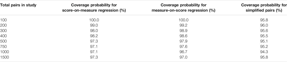
TABLE 1. Coverage probabilities for three methods dependent upon the total number of pairs in the study.

Unlike the other CJ approaches, in the simplified pairs method, we are not attempting to assign CJ measures to representations. As such, we do not calculate any reliability coefficients analogous to the SSR. Rather, the chief way in which we assess the reliability of a simplified pairs study in practice is by looking at the estimated standard errors. With this in mind, it is reassuring that the analysis here suggests we can estimate these accurately.

Conclusion

This paper has reviewed some possible approaches to using expert judgement to equate test versions. In particular, the research has evaluated a new approach (simplified pairs) to this problem and shown via simulation that we expect it to be more efficient than existing alternatives, such as that suggested by Bramley (2005), that rely upon the Bradley-Terry model. Improved efficiency is possible because, by changing the way results are analyzed, we can include a far higher number of representations within data collection without increasing the workload for judges. The simplified pairs approach is also the only approach where we can produce trustworthy confidence intervals for the estimated relative difficulty of two tests.

The analysis has also revealed some weaknesses in the traditional approach based on regression of the scores awarded to representations on measures of holistic quality from a CJ study. In particular, the results indicate that this method is biased towards the difference in the mean scores of the representations selected for the study. Given that the whole point of analysis is to provide fully independent evidence of the relative difficulty of two tests, such biases are undesirable.

The results in this paper suggest that, using a simplified pairs approach, a CJ study based on no more than 300 paired comparisons in total may be sufficient to link scores scales across test versions reasonably accurately. It is worth considering how this workload compares to a more traditional awarding meeting (not based on CJ) where expert judges would attempt to set grade boundaries on 1 year’s exam that maintain standards from previous years. According to Robinson (2007), in the past, traditional awarding meetings in England would generally involve at least eight examiners. In these meetings, each examiner would be expected to review at least seven exam scripts within a range of plus or minus three from a preliminary grade boundary. This process might be repeated for up to three separate grade boundaries (for example, grades A, C and F in England’s GCSE examinations). Thus, a total of 168 (=8 judges*7 scripts per grade*3 grades) script reviews might have taken place within an awarding meeting. With this in mind, it is clear that the current suggestion of a CJ-based process requiring 300 paired comparisons would require more resources than traditional awarding—although not of a vastly increased order of magnitude.

It is worth noting that the suggested method, based on logistic regression, does require a few assumptions. In particular, the suggested logistic regression method assumes a linear relationship between the difference in the raw scores of the representations being compared and the log odds of the representation from a particular test version being judged superior. In addition, the method assumes that the relationship between score differences and judged representation superiority is constant across all of the judges in a study. In practice, both of these assumptions could be tested using the grouping method described in chapter 5 of Hosmer and Lemeshow (2000). If there was any sign of lack of fit then it is fairly straightforward to adjust the model accordingly, for example, by adding additional (non-linear) terms to the logistic regression equation. If there were evidence that results varied between different judges, then it would be possible to use multilevel logistic regression as an alternative with judgements nested within judges to account for this.

This paper has only provided detailed results from one simulation study. However, it is fairly easy to generalize the results to simulations with different parameters. For example:

• We know that the score-on-measure regression method is biased towards the difference in the mean scores of sampled representations from different test versions (zero in our study). As a result, the greater the true difference in difficulty between test versions, the greater the level of bias we’d expect to see.

• By the same logic, if representations were randomly sampled rather than selected to be evenly spaced over the range of available scores, then the mark-on-measure regression method would be biased towards the difference in population means rather than towards zero. In our simulated example this would be an advantage. However, in practice, due to the changing nature of students entering exams in different years the difference in population means may or may not reflect the difference in the difficulty of the two tests. One change from the earlier results would be that, due to random sampling, the standard deviation of estimated differences via score-on-measure regression (e.g., Figure 4) would decrease rather increase with the number of pairs in the study.

• It is also fairly easy to predict the impact on results of reducing the spread of true CJ measures in the simulation. This naturally leads to the estimated CJ measures being less reliable. With estimated CJ measures being less reliable, the bias of the score-on-measure regression method would increase. Aside from this, the reduced reliability of all CJ measures would reduce the stability of all other methods. This includes simplified pairs where the reduced spread of true CJ measures would lead to a weakening of the relationship between score differences and the decisions made by judges – in turn leading to reduced stability in estimates.

Although, for brevity, results are not included in this paper, the suggestions in the above bullets have all been confirmed by further simulations. Whilst it is possible to rerun our simulation with different parameters it is worth noting that the parameters of the simulation presented in this paper have been very carefully chosen to reflect a typical situation that is likely to be encountered in practice. As such, the results that have been presented provide a reasonable picture of the level of accuracy that can be achieved via the use of CJ for linking or equating.

Aside from simulation, demonstrations of the simplified pairs technique in practice can be found in Benton et al. (2020). This includes details on how the method can be extended to allow the difference in the difficulty of two tests to vary across the score range. The combination of theoretical work based on simulation (this current paper) and previous empirical experimental work indicate that simplified pairs provides a promising mechanism by which CJ can inform linking and equating.

Data Availability Statement

The original contributions presented in the study are included in the article/Supplementary Material, further inquiries can be directed to the corresponding author.

Author Contributions

The author confirms being the sole contributor of this work and has approved it for publication.

Conflict of Interest

The author declares that the research was conducted in the absence of any commercial or financial relationships that could be construed as a potential conflict of interest.

Publisher’s Note

All claims expressed in this article are solely those of the authors and do not necessarily represent those of their affiliated organizations, or those of the publisher, the editors and the reviewers. Any product that may be evaluated in this article, or claim that may be made by its manufacturer, is not guaranteed or endorsed by the publisher.

Footnotes

¹Of course, we are still using logistic regression and a Bradley-Terry model is itself a form of logistic regression. However, although they can be thought of in this way, Bradley-Terry models usually make use of bespoke algorithms to address issues that can occur in fitting (e.g., see Hunter, 2004). They also have particular requirements in terms of the data collection design (such as connectivity). All of this is avoided.

²An even spread of 50 values between 20 and 90 is first defined by the sequence of number 20.00, 21.43, 22.86, 24.29,…, 88.57, 90.00. For each of these values in turn, we randomly select one script from those with raw scores as close as possible to these values. That is, from those with raw scores of 20, 21, 23, 24,…,89, 90.

³GCSE stands for General Certificate of Education. GCSEs are high-stakes examinations taken each summer by (nearly) all 16-year-olds in England and OCR is one provider of these examinations. The years 2015 and 2016 were chosen as they were comfortably after the previous set of GCSE reforms and the last year before the next set of GCSE reforms began. As such, they represented the most stable possible pair of years for analysis. Only grades A and C were explored and only examinations that were taken by at least 500 candidates in each year. At grade A the median absolute change in boundaries was 3.8 per cent of marks. At grade C the median absolute change in boundaries was 3.3 per cent of marks.

⁴It is possible to address this issue via the application of multilevel modelling (see Benton et al., 2020, for details). However, this changes the estimates themselves and is beyond the scope of this article so was not considered here.

⁵True reliabilities are calculated as the squared correlation between estimated CJ measures and the true values of CJ measures (i.e., simulated values).

⁶Based on true reliabilities. Note that true reliabilities and scale separation reliabilities were always very close to one another except where the number of comparisons per script was below 5.

References

Allison, P. D., and Christakis, N. A. (1994). Logit Models for Sets of Ranked Items. Sociological Methodol. 24, 199–228. doi:10.2307/270983

CrossRef Full Text | Google Scholar

Benton, T., Cunningham, E., Hughes, S., and Leech, T. (2020). Comparing the Simplified Pairs Method of Standard Maintaining to Statistical equatingCambridge Assessment Research Report. Cambridge, UK: Cambridge Assessment.

Google Scholar

Black, B., and Bramley, T. (2008). Investigating a Judgemental Rank‐ordering Method for Maintaining Standards in UK Examinations. Res. Pap. Edu. 23 (3), 357–373. doi:10.1080/02671520701755440

CrossRef Full Text | Google Scholar

Bradley, R. A., and Terry, M. E. (1952). Rank Analysis of Incomplete Block Designs: The Method of Paired Comparisons. Biometrika 39, 324–345. doi:10.1093/biomet/39.3-4.324

CrossRef Full Text | Google Scholar

Bramley, T. (2005). A Rank-Ordering Method for Equating Tests by Expert Judgment. J. Appl. Meas. 6, 202–223.

Google Scholar

Bramley, T., and Gill, T. (2010). Evaluating the Rank‐ordering Method for Standard Maintaining. Res. Pap. Edu. 25 (3), 293–317. doi:10.1080/02671522.2010.498147

CrossRef Full Text | Google Scholar

Bramley, T. (2015). Investigating the Reliability of Adaptive Comparative JudgmentCambridge Assessment Research Report. Cambridge, UK: Cambridge Assessment.

Google Scholar

Bramley, T., and Vitello, S. (2019). The Effect of Adaptivity on the Reliability Coefficient in Adaptive Comparative Judgement. Assess. Educ.: Princ. Policy Pract. 26 (1), 43–58.

CrossRef Full Text | Google Scholar

Curcin, M., Howard, E., Sully, K., and Black, B. (2019). Improving Awarding: 2018/2019 Pilots. Ofqual Report Ofqual/19/6575. Available at: https://assets.publishing.service.gov.uk/government/uploads/system/uploads/attachment_data/file/851778/Improving_awarding_-_FINAL196575.pdf (Accessed August 11, 2021).

Google Scholar

Everitt, B. S., and Skrondal, A. (2020). The Cambridge Dictionary of Statistics. 4th Edn., Cambridge University Press.

Google Scholar

Hosmer, D. W., and Lemeshow, S. (2000). Applied Logistic Regression. New York: John Wiley & Sons.

Google Scholar

Hunter, D. R. (2004). MM Algorithms for Generalized Bradley-Terry Models. Ann. Stat. 32, 384–406. doi:10.1214/aos/1079120141

CrossRef Full Text | Google Scholar

Plackett, R. L. (1975). The Analysis of Permutations. Appl. Stat. 24, 193–202. doi:10.2307/2346567

CrossRef Full Text | Google Scholar

Pollitt, A. (2012). The Method of Adaptive Comparative Judgement. Assess. Educ. Principles, Pol. Pract. 19 (3), 281–300. doi:10.1080/0969594x.2012.665354

CrossRef Full Text | Google Scholar

Robinson, C. (2007). “Awarding Examination Grades: “Current Processes and Their Evolution,” in Techniques for Monitoring the Comparability of Examination Standards. Editors P. E. Newton, J. Baird, H. Goldstein, H. Patrick, and P. Tymms (London: Qualifications and Curriculum Authority), 97–123.

Google Scholar

Robitzsch, A. (2019). sirt: Supplementary Item Response Theory Models. R Package Version 3.7-40. Available at: https://CRAN.R-project.org/package=sirt.

Google Scholar

Verhavert, S., Bouwer, R., Donche, V., and De Maeyer, S. (2019). A Meta-Analysis on the Reliability of Comparative Judgement. Assess. Educ. Principles, Pol. Pract. 26, 541–562. doi:10.1080/0969594x.2019.1602027

CrossRef Full Text | Google Scholar