
94% of researchers rate our articles as excellent or good
Learn more about the work of our research integrity team to safeguard the quality of each article we publish.
Find out more
ORIGINAL RESEARCH article
Front. Educ., 12 October 2021
Sec. Assessment, Testing and Applied Measurement
Volume 6 - 2021 | https://doi.org/10.3389/feduc.2021.723141
 Robert Trevethan1*
 Kang Ma2
Certain combinations of number and labeling of response options on Likert scales might, because of their interaction, influence psychometric outcomes. In order to explore this possibility with an experimental design, two versions of a scale for assessing sense of efficacy for teaching (SET) were administered to preservice teachers. One version had seven response options with labels at odd-numbered points; the other had nine response options with labels only at the extremes. Before outliers in the data were adjusted, the first version produced a range of more desirable psychometric outcomes but poorer test–retest reliability. After outliers were addressed, the second version had more undesirable attributes than before, and its previously high test–retest reliability dropped to poor. These results are discussed in relation to the design of scales for assessing SET and other constructs as well as in relation to the need for researchers to examine their data carefully, consider the need to address outlying data, and conduct analyses appropriately and transparently.
Ideally, scales based on a Likert format possess a range of desirable attributes. Predominant among these are items not having a narrow range of responses or attracting a large number of outliers; most items being neither positively nor negatively skewed; responses occurring across the full array of response options; moderate interitem correlations as well as other indicators of interitem association being neither too low nor excessively high; and composite scores (as opposed to individual items) having few outliers, not having undesirably narrow standard deviations (SDs) or ranges, not departing severely from normality, and providing a representation of people such that genuine similarities and differences are tapped. Some of these characteristics are related to each other, but another, conceptually separate, psychometric feature is high test–retest reliability.
Our primary aim in this study was to determine whether specific combinations of response options used with Likert-type scales are likely to facilitate or thwart desirable psychometric outcomes. We were prompted by a review article in which DeCastellarnau (2018) examined a range of response option features, including the number and labeling of those options. Having summarized a large corpus of relevant research, DeCastellarnau indicated that further research was needed about a range of issues, including the extent to which “the overlap” (p. 1539) between some aspects of response options might have an impact on data quality—an impact that might be independent of any influence that each variable might exert independently.
In this study, we examined the overlapping effect of number of response options and option labels when assessing sense of efficacy for teaching (SET)1—a topic that we had previously researched in Australia and China (see Ma and Cavanagh, 2018; Ma et al., 2019; Ma and Trevethan, 2020). We had noticed differences in results that we suspected might be attributable to differences in combinations of the response options that we had offered participants. Noticeable among these differences were data skewness as well as the means and SDs of SET scores. We had not explored test–retest reliability, but were curious to see whether it, also, might be influenced by specific combinations of response options.
In order to address our aim with the advantages of an experimental design, we created two versions of a scale to assess SET. Both versions had a Likert format, thus corresponding with the general format used in research about SET since empirical interest in the topic commenced in the mid-1970s (see Armor et al., 1976). The versions differed from each other only with respect to number and labeling of response options. Both of these features have differed widely in research about SET, and it is therefore tempting to investigate whether their combination might have influenced the validity, and ultimately the value, of that body of research.
For the most part, SET has been assessed with the Teacher Sense of Efficacy Scale (TSES; Tschannen-Moran and Hoy, 2001) or close variants of that scale, including translations (see Duffin et al., 2012; Ma et al., 2019). Because of the TSES’s format, nine response options have usually been offered to participants when measuring SET, either because researchers use the TSES itself or, it would appear, because they respect that format (see, e.g., Wolters and Daugherty, 2007; Yin et al., 2017; Cheon et al., 2018). For similar reasons, labels have often been provided above the five odd-numbered options but not above any of the even-numbered options.
Use of nine response options and the above pattern of labeling is far from universal, however. At one extreme, SET has been assessed with only three response options, each of which was labeled (see Shi, 2014), and, at the other extreme, Bandura (2006) created subscales to assess SET with response options ranging from 0 to 100 and labels at only the extremes and midpoint.
In this study, we investigated response-option characteristics that are more typical within research about SET. One version of the scale, which we called Version A, had seven option points with labels above the four odd-numbered options. Our choice of seven options was based on recommendations that the optimal number of options is seven (Carifio and Perla, 2007; Krosnick and Presser, 2010) or either five or seven (Robinson, 2018) as well as the argument that the psychometric properties of scales do not improve with more than seven options (Nunnally, 1978). Placing labels above only the odd-numbered options conformed with the Norwegian Teacher’s Self-Efficacy Scale (Skaalvik and Skaalvik, 2007) and with our own research in China (Ma et al., 2019; Ma and Trevethan, 2020).
The second version of the scale, Version B, had nine response options because the TSES and the newer Scale for Teacher Self-Efficacy (STSE; Pfitzner-Eden et al., 2014) both have that number of options. Unlike the TSES, however, labels for Version B were placed only at the extremes, as in the STSE, because the latter scale’s creators claimed to have improved the TSES. This conformed with the scale used in our previous research in Australia (Ma and Cavanagh, 2018).
We conducted this study in the belief that administering Version A to one group of participants, and Version B to another, highly similar, group of participants, would reveal whether results from one version were more desirable than were results from the other.
Participants came from two separate groups of preservice teachers that, in order to correspond with our naming of the scale versions, we called Group A (n = 40) and Group B (n = 41). They comprised the total enrolment of students within the second-year cohort of the primary teacher education program at a university categorized as a normal university in Jinan, Chinese mainland. The groups had been created when the students commenced their program2, at which time a concerted effort was made to achieve comparability on students’ university entrance examination scores, gender, and sociodemographic variables such as city of origin. Ages in Group A ranged from 18 to 21 years (M = 19.42, SD = 0.59) and in Group B from 19 to 21 years (M = 19.54, SD = 0.60), and the majority were female (82.1% in Group A; 82.9% in Group B).
None of these students had yet experienced teaching placements as part of their course.
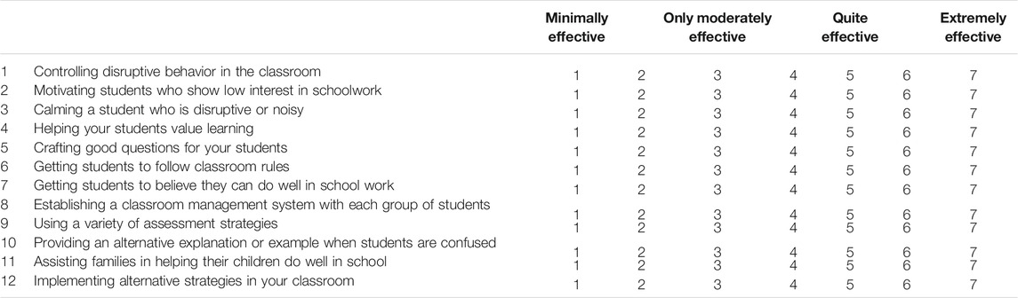
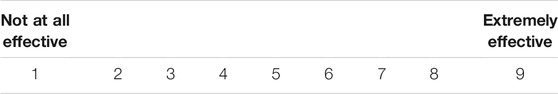
Both versions of the SET scale contained identical instructions and items based on the 12-item short form of the TSES that we had previously translated into Chinese (see Ma et al., 2019). The versions differed only with regard to response options. Version A, with its seven response points, had labels of minimally effective, only moderately effective, quite effective, and extremely effective at points 1, 3, 5, and 7, respectively. Options 2, 4, and 6 were numbered but not labeled. Version B, with its nine response points, had labels of not at all effective and extremely effective at the extremes of 1 and 9, respectively, and Options 2 to 8 were numbered but not labeled.
The full scale for Version A, and the response options for Version B, are provided in the Appendix.
On an initial occasion of administration, participants were asked to indicate their gender and age as well as their favourite movie and favourite primary school teacher—the last two variables intended to maintain participants’ anonymity when retest data were matched. At the second administration, participants were again asked to provide these same two forms of identification.
In parallel lectures, each group of students was initially given verbal information about the research, invited to indicate their willingness to participate, and administered the respective questionnaires. The retest surveys were administered, again in parallel lectures, 3 weeks later. Group A was administered Version A on two occasions (once originally, then again at retest); correspondingly, Group B was administered Version B on two occasions (once originally, then at retest). Questionnaires were administered in hard copy form, and attendance was 100% on all four occasions of measurement. Between administrations, there were no instructional or on-campus practical experiences that were likely to have altered the students’ SET.
On each occasion, one of the participants in Group A chose Option 4 across all items. That participant differed on each occasion, and, when both of those participants’ identical-response records were discarded, Group A was left with 39 participants on each occasion. Of the remaining participants in Group A, seven either failed to provide identification or used different identification on each occasion. Therefore, only 32 participants from Group A were available for test–retest analyses. Of the 41 participants in Group B, six either failed to provide identification or used different identification on each occasion. Therefore, only 35 participants from Group B were available for test–retest analyses.
For each item, means and SDs were calculated in light of the arguments by Hair et al. (2014) that “indicators with ordinal responses of at least four response categories can be treated as interval” (p. 612) and Norman (2010) that calculating means and SDs on ordinal data can “give the right answer even when assumptions are violated” (p. 627). Outliers identified as such by SPSS on individual items were noted. A composite score for each version on each occasion was calculated by obtaining the mean of responses on the 12 items3, thus producing SET values that could range from one to seven on Version A, and from one to nine on Version B. Histogram bins for both versions were set at spans of 0.40. Composite scores were initially inspected for outliers, regarded as any data points within the first or fourth quartiles that exceeded 1.5 x the interquartile range or that departed by ≥ 0.50 from the main body of scores among which there were no differences > 0.50. After an initial set of analyses with composite scores in which outliers were included, we winsorized outliers in those scores and conducted selected analyses again.
We assessed test–retest reliability in four ways. First, for each participant the absolute difference between the composite scores at Times 1 and 2 was calculated, and an independent-samples t-test was used to compare these differences from Group A with those from Group B to identify intraindividual volatility within each version. More conventionally, we also conducted paired-samples t-tests to compare the scores within each group across the two times of administration to detect general upward or downward movement in scores, and within each group we also calculated Pearson’s product-moment correlation coefficients and intraclass correlation coefficients (ICCs; 3,1 [two-way mixed, single measures], absolute agreement; see Trevethan, 2017).
In order to detect whether outliers were likely to distort the test–retest results, particularly Pearson’s correlations and ICCs (see Vaz et al., 2013), we removed composite scores of participants if there were outliers either in their original composite scores or in the absolute difference between their composite scores at the two times of administration, and we then conducted fresh test–retest analyses involving paired-samples t-tests, correlation coefficients, and ICCs.
We assessed normality of distributions by inspecting histograms—a recommended procedure when sample sizes are small (Are the skewness and kurtosis useful statistics?, 2016; Wheeler, 2004). When examining interitem correlations, we followed the recommendation of Clark and Watson (1995) that these correlations ideally lie between 0.15 and 0.50. We also followed the recommendation of Briggs and Cheek (1986) that the mean of these correlations ideally lies between 0.20 and 0.40. We assessed coefficient alphas in relation to the recommendation of McDowell and Newell (1996) that they be moderate and, more specifically, in the region of 0.84 for a scale with 12 items (see Cortina, 1993). When assessing ICCs, we used categories recommended by Portney and Watkins (2019) and Koo and Li (2016). These categories were < 0.50, poor; 0.50 to 0.75, poor to moderate; and ≥ 0.75 to 0.90, good.
Means and SDs for all items are shown in Table 1. On both occasions, the means of responses to individual items were consistently and noticeably lower on Version A than on Version B—a phenomenon that can be easily explained by the highest option on Version A being seven whereas the highest option on Version B was 9.
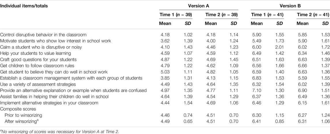
TABLE 1. Means and standard deviations of individual items and composite scores.
Entries in Table 1 also reveal that SDs on individual items were almost always narrower on Version A than they were on Version B. As indicated in Table 2, the mean SD across all items was also narrower on both occasions for Version A than for Version B. Nevertheless, as also indicated in Table 2, none of the individual items exhibited SDs smaller than 1.00.
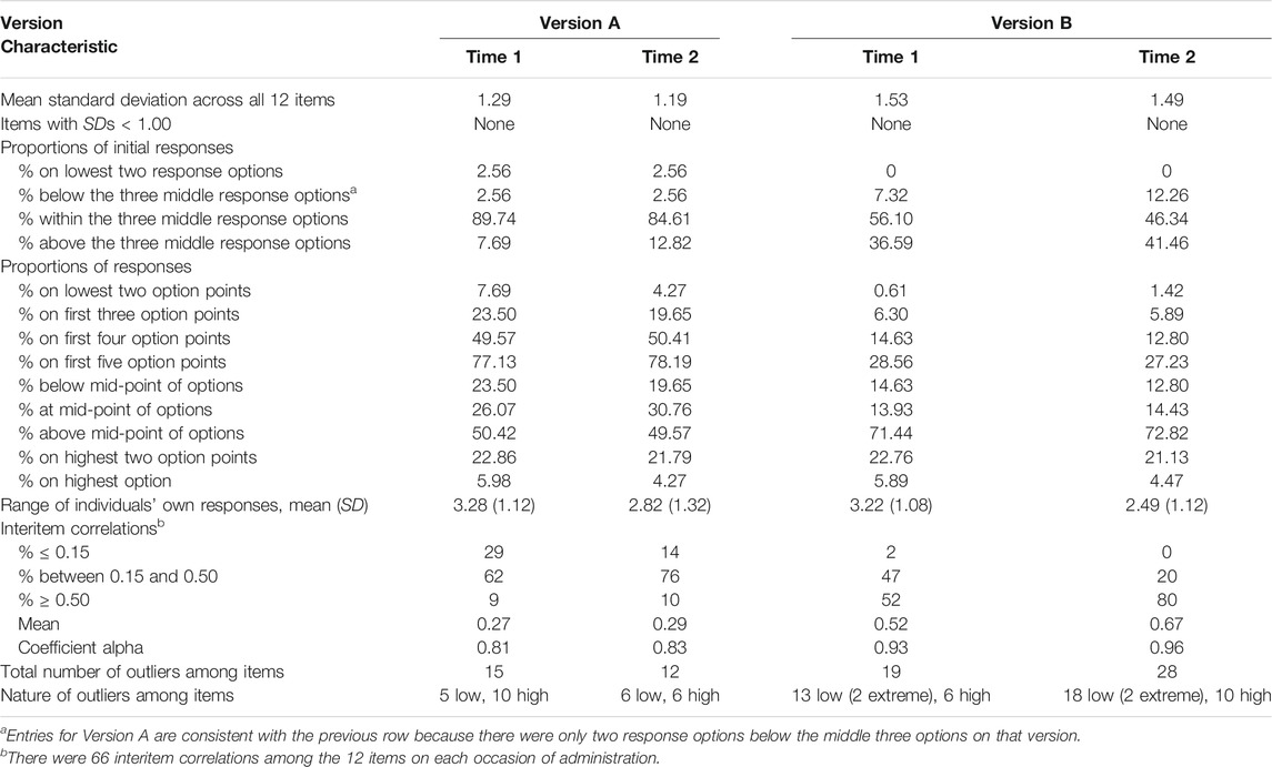
TABLE 2. Miscellaneous results concerning data characteristics.
Entries in Table 2 indicate that, as a response to the first item, most participants in Group A selected one of the three middle options, whereas noticeably fewer participants in Group B used one of the three middle options on the first item. Furthermore, a minimal number of participants on both versions selected an option below the middle three options on the first item; none of the Version B respondents commenced responding on that version’s lowest two options; and a small percentage of Group A selected an option above the middle three on the first item, but a noticeably greater proportion of participants on Version B selected options above the middle three options on the first item. These choices are reflected in the first row of entries in Table 1, where the means of the participants’ first response are shown. The associated SDs, also in the first row of entries in Table 1, indicate that there was greater similarity among responses to the first item on Version A than there was to the first item on Version B.
As shown by entries in Table 2, the lowest two response options were used to only a small extent on Version A and to an even smaller extent on Version B, foreshadowing a degree of negative skewness in relation to the option range on both versions, but more so on Version B. Entries in Table 2 also indicate that on Version A there was a gradual increase in use of the first five response options, but on Version B, use of Options 3 and 4 remained low and it was only by Option 5 (the midpoint) on that version that the cumulative use of options exceeded cumulative use of the first three options of Version A. For Version A, half of the responses fell at or below the option-range midpoint, but for Version B, use of above-midpoint options was particularly noticeable, at more than 70% on both occasions.
On both versions, as indicated by the ranges and SDs of individuals’ responses in Table 2, each participant tended to respond within a limited range of the available options. For example, the SD of 1.12 on Version A at Time 1 indicates each participant tended to respond within a span of only three options. As also indicated in Table 2, most of the 66 interitem correlations on each occasion for Version A fell between 0.15 and 0.50, but most interitem correlations for Version B were ≥ 0.50. For Version A, the mean interitem correlations were 0.27 and 0.29 for Times 1 and 2, respectively; for Version B, the corresponding mean interitem correlations were 0.52 and 0.67 (refer to Table 2). The coefficient alpha values on the two occasions of measurement were 0.81 and 0.83, respectively, for Version A, and were therefore noticeably lower than were the alphas of 0.93 and 0.96 for Version B (refer to Table 2).
Entries in Table 2 also indicate that, among the individual items, there were fewer outliers within the two administrations of Version A (n = 27) than within the two administrations of Version B (n = 47). Furthermore, the number of these outliers was similar on both administrations of Version A but there were noticeably more outliers for Version B at Time 2 than there had been at Time 1, and no outliers on Version A were identified as being extreme by SPSS, but two outliers on both measurement occasions were identified as extreme on Version B.
The penultimate row of entries in Table 1 indicates that, for each version’s composite scores, the SDs were narrower for Version A at each timepoint, and, as shown within the second row of entries in Table 3, the narrower SDs on Version A are reflected in its smaller range of scores.
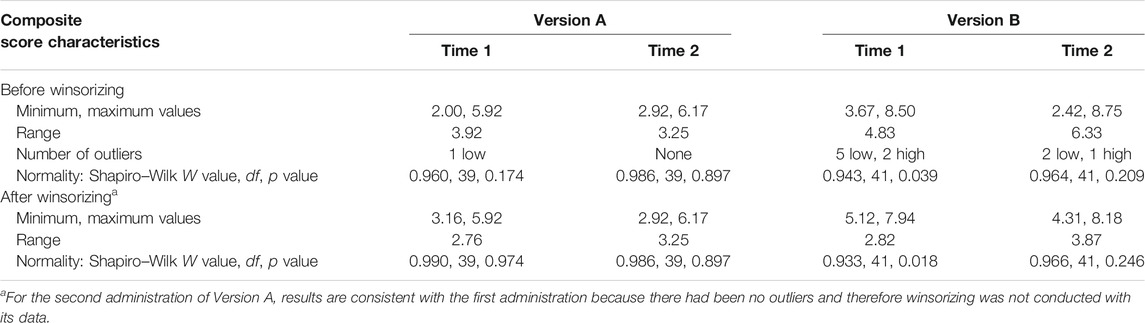
TABLE 3. Results concerning composite scores.
Among the composite scores across the two occasions of administration, there was only one outlier for Version A, but 10 outliers for Version B (refer to third row of entries in Table 3). Not shown in Table 3 is that three of the seven Version B participants with outliers at Time 1 had outlying scores at Time 2, but the remaining four participants did not.
Figure 1 contains histograms showing each version’s composite scores on both measurement occasions. These histograms, each with the normal curve superimposed, suggest satisfactory skewness and kurtosis for Version A on both occasions (Figures 1A,B), with the exception of the single outlier at Time 1.
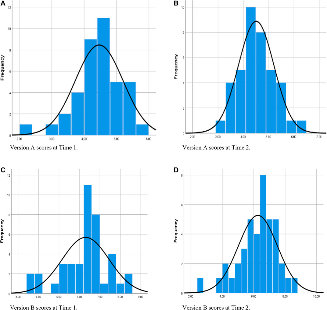
FIGURE 1. Distribution of composite scores on each version on each occasion of measurement prior to winsorizing data.
Figure 1C supports the earlier observation that Version B had a concentration of scores immediately above the response-option midpoint at Time 1; however, the remaining frequencies are revealed to be irregular, and there was a statistically significant departure from normality (refer to Table 3 for Shapiro–Wilk test results). Figure 1D indicates that, at Time 2, the distribution of scores on Version B could be regarded as exhibiting satisfactory skewness and kurtosis apart from some low outliers, but, as at Time 1, most scores lie well above that version’s option-range midpoint.
Several outcomes of winsorizing are indicated in the final row of entries in Table 1, where the means and SDs of composite scores remained very similar or identical across the two administrations of Version A. The means of Version B also changed little after winsorizing, probably because its outliers lay at both ends of its distributions. As also indicated in the final two rows of entries in Table 1, however, the SDs decreased noticeably on Version B as a result of winsorizing. At Time 1, this brought the Version B SD closer to the SDs at both times of administration on Version A.
After winsorizing, data characteristics changed between the two versions in additional ways, as indicated in Table 3. Most noticeably, on Version B the minimum scores increased and maximum scores decreased on both occasions of measurement, and all composite scores exceeded the midpoint of the option range at Time 1. The ranges of scores for Versions A and B across the four administrations became less discrepant (refer to Table 3).
Figure 2 contains histograms showing each version’s composite scores on both occasions of measurement after winsorizing all outliers. These histograms, each again with the normal curve superimposed, indicate bell-shaped distributions for Version A on both occasions of measurement (Figures 2A,B), but for Version B the histograms are again irregular on both occasions (Figures 2C,D)—with peaks and troughs across the full distribution of scores at Time 1, and a noticeable group of low scores at Time 2. As had occurred prior to winsorizing, the Shapiro–Wilk test again indicated a significant departure from normality for Version B at Time 1 (refer to Table 3).
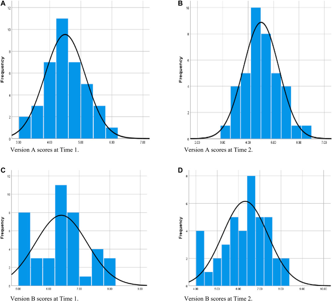
FIGURE 2. Distribution of composite scores on each version on each occasion of measurement after winsorizing data where considered necessary. (Version A at Time 2 was not subjected to winsorizing; it is included in this set of figures to facilitate comparisons.)
Analyses performed specifically to assess test–retest reliability are described in this section and summarized in Table 4.

TABLE 4. Results relevant to test–retest analyses.
As shown in Table 4, the absolute difference of individual participants’ scores between Times 1 and 2 contained two high outliers in the data for Version A and one high outlier in the data for Version B—reflected in SDs and maximum differences. Despite these results, the means of the absolute differences were similar for both versions, as confirmed by an independent-samples t-test, t (65) = 0.25, p = 0.802. Temporal consistency was also reflected in the paired-samples t-tests (reported in Table 4), which indicated that participants’ scores did not increase or decrease significantly on either version across the 3-week period.
In contrast to these similarities in temporal stability for both versions, Pearson’s correlations comparing scores across Times 1 and 2 were 0.56 for Version A and 0.90 for Version B, and the ICCs were 0.57 for Version A and 0.90 for Version B—thus suggesting much greater temporal consistency on Version B. Anomalously, however, comparison of the histograms in Figure 1 reveals Version A to have greater similarity across the two timepoints than did Version B across the two timepoints.
As a consequence of removing records of participants in the retest samples if their original data contained outliers or if there were outliers in their absolute difference scores, data from two Version A participants and six Version B participants were discarded, leaving 30 participants in the former group and 29 in the latter. In test–retest analyses conducted with these more refined samples, the paired-samples t-tests again demonstrated that scores did not move significantly up or down for either version across the 3-week timespan (refer to Table 4). However, prior noticeable differences between the versions no longer existed in that the SDs associated with the t-tests were much more similar both within and between versions, the Pearson’s correlations became almost identical to each other on both versions, as did the ICCs—with both kinds of correlation increasing for Version A and decreasing for Version B (refer to Table 4).
In this case, a comparison of the histograms in Figure 2 is again anomalous in that Version A has an almost identical distribution at each timepoint, but the Version B distributions differ noticeably from one timepoint to the other.
There are several similarities between responses and outcomes on the two scale versions. On both versions, participants tended to constrain themselves to their own, intraindividual and limited, span of option choices that departed only moderately from their first response, and they chose the highest two options to a similar, and moderate, extent. Because nonuse of the lowest two options was much stronger on Version B, respondents on both versions were similar in that they essentially availed themselves of only seven options. Despite the SDs on individual items usually being narrower on Version A, the SDs were satisfactorily wide on both versions’ items. Two of the four test–retest reliability procedures also yielded similar results in that the size of absolute differences in each participant’s scores across the 3-week period did not differ significantly between the versions, and on neither version did scores move significantly either up or down from one timepoint to the other.
In contrast to these similarities, there were a number of differences in data characteristics and indicators of test–retest reliability. Below, we identify these differences and investigate whether they are disconnected and inconsequential or, alternatively, give rise to integrated and extended implications that preference one combination of options over the other.
Prior to winsorizing, most of the differences favored Version A. Responses on that version tended to be evenly distributed around the midpoint of its option range, whereas responses on Version B were not only much more likely to lie above that version’s option-range midpoint but many responses were also concentrated there as a group. For Version B, the lowest two options were essentially superfluous. Most interitem correlations on Version A fell in the desirable low-to-moderate band, whereas most of Version B’s interitem correlations were undesirably high. For Version A, both of the mean interitem correlations fell within the range that we regarded as desirable, whereas both of those correlations were undesirably high on Version B. Furthermore, the two coefficient alphas were acceptable on Version A, but both were undesirably high on Version B. On both occasions of administration, Version A had fewer outliers at item and composite-score levels as well as a normal or near-normal distribution of composite scores, whereas, at Time 1, Version B’s composite-score distribution departed significantly from normality. Throughout all of the above comparisons, results on Version A tended to be similar at both timepoints, but results associated with the composite score for Version B differed across timepoints with regard to SDs, ranges, histogram profiles, number of outliers, and the specific participants with outlying scores—thus demonstrating a high degree of instability on Version B.
In contrast, and also prior to winsorizing, a small number of between-version differences appeared to favor Version B. Specifically, the prospect of effectively discriminating between respondents on that version appeared to be higher because of its broader SDs and ranges on composite scores. In addition, within the test–retest analyses, the Pearson’s correlation and ICC were both high on Version B, but mediocre on Version A.
After winsorizing, the comparative strengths of Version B were either no longer as pronounced as they had been, or no longer existed. For example, on Version B at Time 1, the SD of the composite score became more similar to all four composite-score SDs on Version A. More noticeably, after winsorizing, the composite-score ranges on Version B more closely resembled those on Version A, and the test–retest Pearson’s correlations and ICCs became almost identical for both versions as a result of those metrics rising for Version A but falling for Version B.
Some researchers have argued that more response options permit greater differentiation among participants, presumably because participants’ responses can be more nuanced (see Bandura, 2006; Durksen et al., 2017). There are two indications that this did not occur in our research. First, on both versions, participants tended to constrain their responses within a span of two to four options. Second, the two options at the lower extreme on Version B were almost totally ignored. Overall, therefore, the five lowest options on Version B served much the same purpose as the three lowest options on Version A.
These results support the view that having more than seven response options confers little benefit. Four decades ago, Nunnally (1978) claimed that scales with seven response options reach the limit of reliability. Subsequently, Clark and Watson (1995) argued that increasing the number of response options, for example, to nine points, does not necessarily increase a scale’s reliability or validity and could even reduce validity if respondents are unable to make subtle distinctions, and Krosnick and Presser (2010) have argued that meaningful distinctions are difficult to establish when there are more than seven response options. Lozano et al. (2008) used Monte Carlo simulations to compare scales with different numbers of response options and found that both reliability and validity improved as the number of options increased. However, they concluded that the optimum number of options lies between four and seven and that more than seven options produced minimal improvements to the psychometric properties of a scale.
In the present research, there is even an intriguing possibility that the additional options at the lower end of the continuum on Version B emboldened some of its respondents to feel comfortable commencing their responses below the middle three options but not so far below those options that their choice could be considered extreme. In being different from most of their fellow participants, however, their decision to commence responding that way could simultaneously have been a contributor to wider SDs because their subsequent responses remained at that initial level or were sometimes even lower.
Chang (1994) has discussed some of the above issues in terms of trait variance as opposed to method variance, the latter typifying Version B in this case by being associated with what Chang characterized as a systematic error resulting from the format of a scale rather than from genuine interparticipant differences. Chang referred to the possibility of a greater number of response options leading to “a systematic “abuse” of the scale” (p. 212)—a possibility that appears to have been manifested in Version B and might simply be conceived of as measurement error.
The different patterns of responses on the two versions strongly suggest that labels provide respondents with information about where to commence, and continue, responding. The clearest evidence of this is the large majority of respondents on Version A initially choosing one of the three central response options, the outer two of which were labeled. Because all respondents tended to continue responding close to their initial response, most composite scores on Version A fell between the labels only moderately effective and quite effective—indicating what could well be an appropriate target for responses given that undergraduate students of education might reasonably carry cautious optimism regarding their SET, particularly if teaching practicums had not yet been part of their course. In contrast, responses on Version B were more disparate across the option continuum. Labels therefore seem to have provided respondents with semantic focus.
If option labels carry this advantage, the wider SDs on Version B could be largely attributed to participants beginning to respond at more discrepant points on the option continuum in the absence of meaningful support, and then continuing to respond within a closely related band of options. This tendency, in turn, could have increased the likelihood of outliers that further widened the SDs on Version B. These wider SDs are therefore likely not to reflect genuine interparticipant differences in SET but to have been generated primarily by lack of labels.
Because the distribution of scores on Version B differed between the two times of administration, there is further reason to mistrust interparticipant differences on that version. Even subsequent to winsorizing, there were wider SDs on Version B, and therefore the problems associated with minimal labeling appear to be endemic. Discounting Version B’s wider SDs, therefore, not only removes one of the few advantages that Version B seemed to have over Version A (the ability to distinguish between participants) but reveals Version B to be a trap for unwary researchers because its apparently greater ability to discriminate between respondents is likely to be spurious.
Even the prospect of greater interparticipant variability on Version B because of its wider SDs is called into question by Figures 1C,D with their high concentration of scores immediately above the middle three options. Distinguishing many participants from each other within those predominant groups would have been no easier, and perhaps even more difficult, than distinguishing between many participants on Version A.
Some results in this study appear to be directly related to the differences in response dispersion, particularly in relation to outliers. The larger number of outliers among Version B’s items could have contributed to the excessively high coefficient alphas on that version, consistent with Liu et al. (2010) having demonstrated that outliers “severely inflated” alphas on data obtained from Likert-type scales (p. 5). Asymmetry among the outliers on Version B could also have contributed to its high alphas (see Liu and Zumbo, 2007). These undesirably high alphas could therefore be relegated to the status of statistical artifacts that cast Version B in an unfavorable light prior to winsorization.
When assessing test–retest reliability prior to winsorization, the correlations and ICCs preferenced Version B over Version A. However, for both versions these results were probably also contaminated by statistical artifacts. On the one hand, lack of variability in data, as there was in Version A, depresses correlation coefficients (Chang, 1994; Goodwin and Leech, 2006) and ICCs (Koo and Li, 2016). On the other hand, Vaz et al. (2013) have demonstrated that both Pearson’s correlations and ICCs are influenced by outliers, which were more prevalent on Version B. These phenomena are likely to explain why, after removal of data from participants with outliers, the Pearson’s correlations and ICCs were almost identical for both versions. Judiciously discarding extreme scores to increase the validity of metrics concerning test–retest reliability for measurement of SET is supported by Osborne and Overbay (2004) and Zijlstra et al. (2007), who argued that removal of outliers is likely to produce results that most accurately represent the population being studied.
The most salient implication arising from this research is that measurement of SET is more likely to be reliable and valid when based on a 7-point option range with labels at the odd-numbered points than when based on a 9-point option range with labels at only the outer extremes. In addition, however, we believe it is evident that researchers should inspect their data for outliers (see Liu et al., 2010), adjust those data if doing so appears to be advisable (see Osborne and Overbay, 2004), and report any difference in outcomes transparently (see Van den Broeck et al., 2005; Zijlstra et al., 2011; Aguinis et al., 2013).
Results from this study also raise serious concerns about the extent to which outliers and invalid score dispersion might distort results and interpretations in other studies. Zijlstra et al. (2011) pointed out that outliers can produce biased estimates in regression analyses as well as distortions to correlations and coefficient alphas. More troubling is Goodwin and Leech (2006) having stated that outliers can affect the whole family of statistics related to correlation, including regression, factor analysis, and structural equation modelling; Chan (1998) having written that “no amount of sophistication in an analytic model can turn invalid inferences resulting from inadequate design, measurement, or data into valid inferences” (p. 475); and Ployhart and Ward (2011) referring to “powerful methodologies [being used] on rather pedestrian data” (p. 420).
This could have particular relevance for the measurement of SET. For example, we have demonstrated that a variety of findings exist concerning the TSES and its close variants with regard to both number and composition of domains in factor analyses (Ma et al., 2019). This variety of findings might to some extent be produced by distorted, even deficient, data—including outliers—that vary from sample to sample. Liu et al. (2012) have indicated that magnitude and number of outliers can inflate or deflate the number of factors produced in factor analysis.
Outlier influence could also raise serious concerns about the validity of test–retest reliability when examining SET. Although scores on Version B differed across the two times of measurement in a number of respects and strongly indicate that responses on that version were undesirably inconsistent, the initial Pearson’s correlation and ICC in the test–retest analyses suggest a high degree of consistency. However, when outliers were addressed, those correlations dropped to become only moderate on Version B, and they rose noticeably on Version A to the point that both versions’ retest correlations were almost identical.
This study could be regarded as limited by being restricted to only a small number of specific participants (one cohort of Chinese undergraduates). However, using these participants permitted a high degree of matching and therefore any differences in the results could be confidently attributed to differences in the response options. Furthermore, parallel results emerge in other studies with larger and more diverse samples. For example, when we used a scale similar to Version A in research with samples of 366 preservice and 276 inservice teachers from China (Ma and Trevethan, 2020), the means of their SET scores also lay close to the option-range midpoint. So, also, did the means of 246 Norwegian inservice teachers on several SET subscales in research by Skaalvik and Skaalvik (2007) and the means of 348 Italian inservice teachers in research by Avanzi et al. (2013)—with both studies having the same combination of response options as Version A.
Conversely, mean SET scores were noticeably higher than the option-range midpoint when scales similar to Version B had been used in research with 90 preservice teachers from Australia (Ma and Cavanagh, 2018) as well as with 640 preservice teachers from Germany and 131 from New Zealand (Pfitzner-Eden et al., 2014), 438 preservice teachers from Germany (Pfitzner-Eden, 2016), and 342 preservice teachers from Germany (Depaepe and König, 2018).
Furthermore, in the studies by Pfitzner-Eden et al. (2014) and Pfitzner-Eden (2016), both of which had response options similar to Version B, most SDs based on composite scores were broad, as had been the composite-score SDs on Version B in our study prior to winsorization. In addition, the coefficient alpha values in the Pfitzner-Eden et al. (2014) and Pfitzner-Eden (2016) research were comparable to the high alpha values in this study before we winsorized the outliers.
It is therefore difficult to regard the findings in this research as attributable to chance resulting from small sample sizes: Similar results are evident in research with much larger samples.
Another possible limitation is this study being based on the specific construct of SET. However, this construct has maintained a considerable prominence in research about teachers and teacher education in the last 4 decades (see Ma et al., 2019), so efforts to improve its measurement are worth pursuing. Furthermore, a number of principles highlighted by this research could well have general applicability, and therefore combinations of number and labeling of response options might not have trivial and inconsequential outcomes but, rather, outcomes that are substantial and substantive across a range of contexts. Furthermore, we have been able to provide other researchers with parameters that might be taken into account when considering the interaction of response options in their own research lest data that are actually not good, appear to be good. In addition, this study demonstrates that researchers should examine their data carefully; allow that examination to inform their analyses in ways that are appropriate and transparent, particularly in relation to outlying data; and adapt scales if doing so is likely to produce data of higher quality.
The raw data supporting the conclusions of this article will be made available by the authors, without undue reservation.
Ethics review and approval were not required for this study to satisfy local legislation and institutional requirements. The students were made aware that participation was not compulsory, and they were also assured that the responses they provided would remain anonymous.
RT and KM worked jointly on preparation of the surveys and data analysis. RT wrote most of the article, and KM provided detailed feedback on successive versions of the text.
The authors declare that the research was conducted in the absence of any commercial or financial relationships that could be construed as a potential conflict of interest.
All claims expressed in this article are solely those of the authors and do not necessarily represent those of their affiliated organizations, or those of the publisher, the editors and the reviewers. Any product that may be evaluated in this article, or claim that may be made by its manufacturer, is not guaranteed or endorsed by the publisher.
Dr Shuhong Lu distributed the surveys for this research, collated the data, and provided detailed information about the participants’ backgrounds.
1Sense of efficacy for teaching, often referred to as teacher sense of efficacy or teacher self-efficacy and therefore abbreviated as TSE, refers to the beliefs held by individuals about their effectiveness in classroom contexts with regard to student instruction as well as management of student behaviour (see Tschannen-Moran and Hoy, 2001; Ma et al., 2019).
2Separate groups were created primarily to facilitate administrative and educational processes.
3Although the TSES is often regarded as comprising three factors, the original publication concerning the TSES (Tschannen-Moran and Hoy, 2001) clearly indicated that only one factor existed in data from PSTs. In addition, in the review section of one of our publications (Ma et al., 2019), we cited studies from the United States and Australia in which PSTs’ data had only one factor, and the empirical component of that publication indicated strongly that both preservice and inservice teachers in China regarded the TSES items as comprising a single factor on both the long and short forms of the scale—possibly resulting from a disinclination to compartmentalize among people from cultures with a Confucian orientation. We therefore feel confident about the validity of adding responses across all 12 TSES short-form items in this research.
Aguinis, H., Gottfredson, R. K., and Joo, H. (2013). Best-Practice Recommendations for Defining, Identifying, and Handling Outliers. Organizational Res. Methods 16 (2), 270–301. doi:10.1177/1094428112470848
Are the skewness and kurtosis useful statistics? (2016). Available at: https://www.spcforexcel.com/knowledge/basic-statistics/are-skewness-and-kurtosis-useful-statistics (Accessed September 13, 2021.
Armor, D., Conroy-Oseguera, P., Cox, M., King, N., McDonnell, L., Pascal, A., et al. (1976). Analysis of the School Preferred Reading Programs in Selected Los Angeles Minority Schools. REPORT NO. R-2007-LAUSD. RAND Corporation (ERIC Document Reproduction Service No. 130 243)
Avanzi, L., Miglioretti, M., Velasco, V., Balducci, C., Vecchio, L., Fraccaroli, F., et al. (2013). Cross-validation of the Norwegian Teacher's Self-Efficacy Scale (NTSES). Teach. Teach. Educ. 31, 69–78. doi:10.1016/j.tate.2013.01.002
Bandura, A. (2006). “Guide for Constructing Self-Efficacy Scales,” in Self-Efficacy Beliefs of Adolescents. Editors F. Pajares, and T. Urdan (Greenwich, CT: Information Age Publishing), Vol. 5, 307–337.
Briggs, S. R., and Cheek, J. M. (1986). The Role of Factor Analysis in the Development and Evaluation of Personality Scales. J. Personal. 54 (1), 106–148. doi:10.1111/j.1467-6494.1986.tb00391.x
Carifio, J., and Perla, R. J. (2007). Ten Common Misunderstandings, Misconceptions, Persistent Myths and Urban Legends about Likert Scales and Likert Response Formats and Their Antidotes. J. Soc. Sci. 3 (3), 106–116. doi:10.3844/jssp.2007.106.116
Chan, D. (1998). The Conceptualization and Analysis of Change over Time: An Integrative Approach Incorporating Longitudinal Mean and Covariance Structures Analysis (LMACS) and Multiple Indicator Latent Growth Modeling (MLGM). Organizational Res. Methods 1 (4), 421–483. doi:10.1177/109442819814004
Chang, L. (1994). A Psychometric Evaluation of 4-Point and 6-Point Likert-Type Scales in Relation to Reliability and Validity. Appl. Psychol. Meas. 18 (3), 205–215. doi:10.1177/014662169401800302
Cheon, S. H., Reeve, J., Lee, Y., and Lee, J.-W. (2018). Why Autonomy-Supportive Interventions Work: Explaining the Professional Development of Teachers' Motivating Style. Teach. Teach. Educ. 69, 43–51. doi:10.1016/j.tate.2017.09.022
Clark, L. A., and Watson, D. (1995). Constructing Validity: Basic Issues in Objective Scale Development. Psychol. Assess. 7 (3), 309–319. doi:10.1037/1040-3590.7.3.309
Cortina, J. M. (1993). What Is Coefficient Alpha? An Examination of Theory and Applications. J. Appl. Psychol. 78 (1), 98–104. doi:10.1037/0021-9010.78.1.98
DeCastellarnau, A. (2018). A Classification of Response Scale Characteristics that Affect Data Quality: A Literature Review. Qual. Quant. 52, 1523–1559. Available at: https://link.springer.com/10.1007/s11135-017-0533-4. doi:10.1007/s11135-017-0533-4
Depaepe, F., and König, J. (2018). General Pedagogical Knowledge, Self-Efficacy and Instructional Practice: Disentangling Their Relationship in Pre-Service Teacher Education. Teach. Teach. Educ. 69, 177–190. doi:10.1016/j.tate.2017.10.003
Duffin, L. C., French, B. F., and Patrick, H. (2012). The Teachers' Sense of Efficacy Scale: Confirming the Factor Structure with Beginning Pre-service Teachers. Teach. Teach. Educ. 28 (6), 827–834. doi:10.1016/j.tate.2012.03.004
Durksen, T. L., Klassen, R. M., and Daniels, L. M. (2017). Motivation and Collaboration: The Keys to a Developmental Framework for Teachers' Professional Learning. Teach. Teach. Educ. 67, 53–66. doi:10.1016/j.tate.2017.05.011
Goodwin, L. D., and Leech, N. L. (2006). Understanding Correlation: Factors that Affect the Size of R. J. Exp. Educ. 74 (3), 249–266. doi:10.3200/JEXE.74.3.249-266
Hair, J. F., Black, W. C., Babin, B. J., and Anderson, R. E. (2014). “Confirmatory Factor Analysis,” in Multivariate Data Analysis. Editors J. F. HairJr., W. C. Black, B. J. Babin, and R. E. Anderson. 7th Edn. (Harlow, United Kingdom: Pearson), 599–638.
Koo, T. K., and Li, M. Y. (2016). A Guideline of Selecting and Reporting Intraclass Correlation Coefficients for Reliability Research. J. Chiropr. Med. 15 (2), 155–163. doi:10.1016/j.jcm.2016.02.012
Krosnick, J., and Presser, S. (2010). “Question and Questionnaire Design,” in Handbook of Survey Research. Editors P. V. Marsden, and J. D. Wright. 2nd Edn. (Bingley, United Kingdom: Emerald), 263–313.
Liu, Y., Wu, A. D., and Zumbo, B. D. (2010). The Impact of Outliers on Cronbach's Coefficient Alpha Estimate of Reliability: Ordinal/Rating Scale Item Responses. Educ. Psychol. Meas. 70 (1), 5–21. doi:10.1177/0013164409344548
Liu, Y., and Zumbo, B. D. (2007). The Impact of Outliers on Cronbach's Coefficient Alpha Estimate of Reliability: Visual Analogue Scales. Educ. Psychol. Meas. 67 (4), 620–634. doi:10.1177/0013164406296976
Liu, Y., Zumbo, B. D., and Wu, A. D. (2012). A Demonstration of the Impact of Outliers on the Decisions about the Number of Factors in Exploratory Factor Analysis. Educ. Psychol. Meas. 72 (2), 181–199. doi:10.1177/0013164411410878
Lozano, L. M., García-Cueto, E., and Muñiz, J. (2008). Effect of the Number of Response Categories on the Reliability and Validity of Rating Scales. Methodology 4 (2), 73–79. doi:10.1027/1614-2241.4.2.73
Ma, K., and Cavanagh, M. S. (2018). Classroom Ready? Pre-Service Teachers' Self-Efficacy for Their First Professional Experience Placement. Aust. J. Teach. Educ. 43 (7), 134–151. doi:10.14221/ajte.2018v43n7.8
Ma, K., and Trevethan, R. (2020). Efficacy Perceptions of Preservice and Inservice Teachers in China: Insights Concerning Culture and Measurement. Front. Educ. China 15 (2), 332–368. doi:10.1007/s11516-020-0015-7
Ma, K., Trevethan, R., and Lu, S. (2019). Measuring Teacher Sense of Efficacy: Insights and Recommendations Concerning Scale Design and Data Analysis from Research with Preservice and Inservice Teachers in China. Front. Educ. China 14 (4), 612–686. doi:10.1007/s11516-019-0029-1
McDowell, I., and Newell, C. (1996). Measuring Health: A Guide to Rating Scales and Questionnaires. 2nd ed. New York, NY: Oxford University Press.
Norman, G. (2010). Likert Scales, Levels of Measurement and the “Laws” of Statistics. Adv. Health Sci. Educ. Theor. Pract 15 (5), 625–632. doi:10.1007/s10459-010-9222-y
Osborne, J. W., and Overbay, A. (2004). The Power of Outliers (And Why Researchers Should ALWAYS Check for Them). Pract. Assess. Res. Eval. 9 (6), 1–12. Available at: https://pareonline.net/getvn.asp?v=9&n=6. doi:10.7275/qf69-7k43
Pfitzner-Eden, F. (2016). I Feel Less Confident So I Quit? Do True Changes in Teacher Self-Efficacy Predict Changes in Preservice Teachers' Intention to Quit Their Teaching Degree. Teach. Teach. Educ. 55, 240–254. doi:10.1016/j.tate.2016.01.018
Pfitzner-Eden, F., Thiel, F., and Horsley, J. (2014). An Adapted Measure of Teacher Self-Efficacy for Preservice Teachers: Exploring its Validity across Two Countries. Z. für Pädagogische Psychol. 28 (3), 83–92. doi:10.1024/1010-0652/a000125
Ployhart, R. E., and Ward, A.-K. (2011). The “Quick Start Guide” for Conducting and Publishing Longitudinal Research. J. Bus. Psychol. 26 (4), 413–422. doi:10.1007/s10869-011-9209-6
Portney, L. G., and Watkins, M. P. (2019). Foundations of Clinical Research: Applications to Practice. 4th ed. Upper Saddle River, NJ: Prentice-Hall.
Robinson, M. A. (2018). Using Multi-Item Psychometric Scales for Research and Practice in Human Resource Management. Hum. Resour. Manage. 57 (3), 739–750. doi:10.1002/hrm.21852
Shi, Q. (2014). Relationship between Teacher Efficacy and Self-Reported Instructional Practices: an Examination of Five Asian Countries/Regions Using TIMSS 2011 Data. Front. Educ. China 9 (4), 577–602. doi:10.1007/BF03397041
Skaalvik, E. M., and Skaalvik, S. (2007). Dimensions of Teacher Self-Efficacy and Relations with Strain Factors, Perceived Collective Teacher Efficacy, and Teacher Burnout. J. Educ. Psychol. 99 (3), 611–625. doi:10.1037/0022-0663.99.3.611
Trevethan, R. (2017). Intraclass Correlation Coefficients: Clearing the Air, Extending Some Cautions, and Making Some Requests. Health Serv. Outcomes Res. Method 17 (2), 127–143. doi:10.1007/s10742-016-0156-6
Tschannen-Moran, M., and Hoy, A. W. (2001). Teacher Efficacy: Capturing an Elusive Construct. Teach. Teach. Educ. 17 (7), 783–805. doi:10.1016/S0742-051X(01)00036-1
Van den Broeck, J., Cunningham, S. A., Eeckels, R., and Herbst, K. (2005). Data Cleaning: Detecting, Diagnosing, and Editing Data Abnormalities. Plos Med. 2 (10), e267. doi:10.1371/journal.pmed.0020267
Vaz, S., Falkmer, T., Passmore, A. E., Parsons, R., and Andreou, P. (2013). The Case for Using the Repeatability Coefficient when Calculating Test-Retest Reliability. PLoS One 8 (9), e73990. doi:10.1371/journal.pone.0073990
Wheeler, D. J. (2004). Advanced Topics in Statistical Process Control: The Power of Shewhart’s Charts. 2nd ed. Knoxville, TN: SPC Press.
Wolters, C. A., and Daugherty, S. G. (2007). Goal Structures and Teachers' Sense of Efficacy: Their Relation and Association to Teaching Experience and Academic Level. J. Educ. Psychol. 99 (1), 181–193. doi:10.1037/0022-0663.99.1.181
Yin, H., Huang, S., and Lee, J. C. K. (2017). Choose Your Strategy Wisely: Examining the Relationships between Emotional Labor in Teaching and Teacher Efficacy in Hong Kong Primary Schools. Teach. Teach. Educ. 66, 127–136. doi:10.1016/j.tate.2017.04.006
Zijlstra, W. P., van der Ark, L. A., and Sijtsma, K. (2007). Outlier Detection in Test and Questionnaire Data. Multivariate Behav. Res. 42 (3), 531–555. doi:10.1080/00273170701384340
Zijlstra, W. P., van der Ark, L. A., and Sijtsma, K. (2011). Outliers in Questionnaire Data. J. Educ. Behav. Stat. 36 (2), 186–212. Available at: https://www.jstor.org/stable/29789477. doi:10.3102/1076998610366263
Keywords: Likert scale, response options, scale options, teacher self-efficacy, teacher sense of efficacy
Citation: Trevethan R and Ma K (2021) Influence of Response-Option Combinations when Measuring Sense of Efficacy for Teaching: Trivial, or Substantial and Substantive?. Front. Educ. 6:723141. doi: 10.3389/feduc.2021.723141
Received: 10 June 2021; Accepted: 13 September 2021;
Published: 12 October 2021.
Edited by:
Sina Hafizi, University of Manitoba, CanadaReviewed by:
Rafael Burgueno, Universidad Isabel I de Castilla, SpainCopyright © 2021 Trevethan and Ma. This is an open-access article distributed under the terms of the Creative Commons Attribution License (CC BY). The use, distribution or reproduction in other forums is permitted, provided the original author(s) and the copyright owner(s) are credited and that the original publication in this journal is cited, in accordance with accepted academic practice. No use, distribution or reproduction is permitted which does not comply with these terms.
*Correspondence: Robert Trevethan, cm9iZXJ0cmV2ZXRoYW5AZ21haWwuY29t
Disclaimer: All claims expressed in this article are solely those of the authors and do not necessarily represent those of their affiliated organizations, or those of the publisher, the editors and the reviewers. Any product that may be evaluated in this article or claim that may be made by its manufacturer is not guaranteed or endorsed by the publisher.
Research integrity at Frontiers
Learn more about the work of our research integrity team to safeguard the quality of each article we publish.