 Shenghai Dai
 Thao Thu Vo1
 Olasunkanmi James Kehinde
 Haixia He
 Cihan Demir
- 1Department of Kinesiology and Educational Psychology, Washington State University, Pullman, WA, United States
- 2Department of Teaching and Learning, Washington State University, Pullman, WA, United States
- 3Pearson VUE, Bloomington, MN, United States
The implementation of polytomous item response theory (IRT) models such as the graded response model (GRM) and the generalized partial credit model (GPCM) to inform instrument design and validation has been increasing across social and educational contexts where rating scales are usually used. The performance of such models has not been fully investigated and compared across conditions with common survey-specific characteristics such as short test length, small sample size, and data missingness. The purpose of the current simulation study is to inform the literature and guide the implementation of GRM and GPCM under these conditions. For item parameter estimations, results suggest a sample size of at least 300 and/or an instrument length of at least five items for both models. The performance of GPCM is stable across instrument lengths while that of GRM improves notably as the instrument length increases. For person parameters, GRM reveals more accurate estimates when the proportion of missing data is small, whereas GPCM is favored in the presence of a large amount of missingness. Further, it is not recommended to compare GRM and GPCM based on test information. Relative model fit indices (AIC, BIC, LL) might not be powerful when the sample size is less than 300 and the length is less than 5. Synthesis of the patterns of the results, as well as recommendations for the implementation of polytomous IRT models, are presented and discussed.
Introduction
The implementation of polytomous item response theory (IRT) models to inform instrument design and validation has been increasing across social and educational contexts where rating scales are usually used (e.g., Carle et al., 2009; Sharkness and DeAngelo, 2011; Cordier et al., 2019; French and Vo, 2020). Examples include the use of polytomous IRT to develop parallel and short forms of existing measures (e.g., Uttaro and Lehman, 1999) and to detect items that show different item functioning (DIF; e.g., Eichenbaum, et al., 2019; French and Vo, 2020).
In practice, the most commonly used polytomous IRT models include the graded response model (GRM; Samejima, 1969) and the generalized partial credit model (GPCM; Muraki, 1992). Compared to the traditional linear factor analytic (FA) approach intended for continuous variables, the IRT models are developed specifically for nominal and ordinal variables (e.g., rating scales). For instance, Maydeu-Olivares et al. (2011) suggested that IRT models yielded better model-data fits than FA models when the data are polytomous ordinal because they involve a higher number of parameters. In addition to the conventional overall model fit and item parameters, the IRT modeling also generates other statistics such as item information and model fit at the person level that are useful in the process of instrument development (see Glockner-Rist and Hoijtink, 2003 and Raju et al., 2002 for further discussions regarding the comparison between FA and IRT). Further, polytomous IRT is the major technique used in computer adaptive tests, allowing for the options of online adaptive measures that use rating scales such as the Likert-type questions across contexts.
Despite the promising use of the polytomous IRT models for instrument development (Penfield, 2014), their performance has not been fully evaluated, especially in the presence of short instrument length (e.g., three items, OECD, 2021), small sample size (e.g., N < 200, Finch & French, 2019), and missing data—characteristics common with rating scales. In achievement tests such as large-scale assessment programs where the IRT models are mainly applied, it is typical to find sufficient instrument or test lengths (e.g., J > 10 items) and relatively large sample sizes (e.g., N ≥ 500), as evidenced by many previous studies that examined the performance of polytomous IRT models (e.g., Reise and Yu, 1990; Penfield and Bergeron, 2005; Liang and Wells, 2009; Jiang et al., 2016). However, it is not uncommon that some instruments with rating scales have as few as three items and are responded by a relatively small number of respondents. For instance, the GPCM has been used by the Programme for International Student Assessment (PISA) to provide validity support for the contextual factors (i.e., derived variables; OECD, 2021) and many of these factors consisted of three to five items such as the perceived feedback—a three-item measure. Examples of small sample sizes include Muis et al. (2009) and Cordier et al. (2019) which reported sample sizes of 217 and 342, respectively, in the application of the polytomous IRT models. In the literature, to the best of our knowledge, there are only three studies that examined the performance of polytomous IRT models with instrument lengths shorter than 10 items across various sample sizes (i.e., Kieftenbeld and Natesan, 2012 [GRM, J = 5–20, N = 75–1,000]; Luo, 2018 [GPCM, J = 5–20, N = 500–2000; Penfield and Bergeron, 2005 [GPCM, J = 6–24, N = 1,000]; see the next section for a detailed review of existing literature). There is no systematic examination on the application of IRT to rating scales across the aforementioned conditions. Further, no studies were identified to evaluate the impact of missing data in the implementation of polytomous IRT models with rating scale data.
In light of this, the purpose of our study is to extend the current literature by systematically examining the performance of GRM and GPCM with rating scale data in the presence of short instrument lengths, small sample sizes, and missing data to various extent. We will also take into account item quality (i.e., item discrimination) in the study.
Background and Literature
Graded Response Model
GRM (Samejima, 1969) is one of the most commonly used polytomous IRT models. It extends the dichotomous two-parameter logistic (2PL) IRT model by allowing ordered and polytomous item responses. As polytomous items have more than two response categories, the response category function is determined explicitly based on the number of response categories (Nering and Ostini, 2011). That is, unlike the 2PL dichotomous IRT models in which only one item difficulty parameter is defined, the GRM specifies category boundary and threshold parameters for the items according to the number of response categories. Specifically, for an item with K response categories, a number of K-1 threshold parameters will be specified in GRM. For instance, an item with four response categories would have three threshold parameters. Below is the equation of GRM (Embretson and Reise, 2000):
where
The threshold parameters in a GRM are calculated cumulatively by modeling the probability that an individual will respond to a given response category or higher (Penfield, 2014). For example, an item with four response categories (e.g., never, sometimes, often, and always) is indicated by Y = 0, 1, 2, 3, showing an ordered level of a latent trait or construct. Then in GRM, three transition steps are used to obtain the three threshold parameters using 2PL dichotomous IRT models that model 1) probability of responding to categories 1 to 3 as compared to category 0 (PY=1,2,3 vs. PY=0), 2) PY=2,3 vs. PY=0,1, and 3) PY=3 vs. PY=0,1,2. Technically, the GRM is usually referred to as a cumulative model (Penfield, 2014) and an “indirect” model (Embretson and Reise, 2000) because of the cumulative nature of the model and the fact that it takes a two-step process to estimate the parameters. Similar to the 2PL dichotomous models, GRM includes only one discrimination parameter for each item (for more technical details of GRM, see Embretson and Reise, 2000; De Ayala, 2013; Penfield, 2014).
Applications of GRM have been gaining attention in survey studies to inform instrument development, evaluation, and revision (e.g., Uttaro and Lehman, 1999; Langer et al., 2008; Carle et al., 2009; Sharkness and DeAngelo, 2011; French and Vo, 2020; Fung et al., 2020). For instance, Uttaro and Lehman (1999) used GRM to analyze the Quality of Life Interview scale and developed three 17-item parallel forms of the instrument, as well as a 10-item short form, for the same construct. Carle et al. (2009) applied GRM to United States (U.S.) National Survey of Student Engagement (NSSE) data and evaluated the psychometric properties of the three student engagement measures, namely student-faculty engagement (five items), community-based activities (four items), and transformational learning opportunities (six items). Their findings demonstrated by the GRM results suggested that the three scales offered adequate construct validity and measured related but separable constructs. Another example is Sharkness and DeAngelo (2011), in which the authors examined the psychometric utility of GRM for instrument construction with data from the U.S. 2008 Your First College Year (YFCY) survey data. In addition to its application in instrument construction and development, GRM has been used for other purposes such as differential item functioning (DIF) detection. For instance, French and Vo (2020) used GRM to investigate DIF between White, Black, and Hispanic youth on a risk assessment. A convenience sample of over 1,400 adolescents responded to a 4-point rating scale. A GRM was used to estimate each of the six subdomains, respectively. Explicitly, the instrument length of the subdomains ranged from five to eight items each, with a total of 40 items. Though not a direct application of GRM, Edelen & Reeve (2007) provided an example of how GRM can be used for questionnaire development, evaluation, and refinement in a behavioral health context. A 19-item Feelings Scale for Depression was evaluated with the data from a national longitudinal study. The results were also used to construct a 10-item short form that had a high correlation with the original form (r = 0.96).
Generalized Partial Credit Model
Another popular polytomous IRT model is GPCM (Muraki, 1992). It extends the partial credit model (Masters, 1982) by introducing a discrimination parameter that varies across items. Although both GPCM and GRM include the same number of parameters, including item discrimination, item step/threshold, and person/theta parameters, they model the response data in a different fashion. Unlike GRM, GPCM is a direct or adjacent category model (Embretson and Reise, 2000; Penfield, 2014) in which the probability of responding to a specific response category is modeled directly (see the model equation below).
where k is a specific response category in the vector of 0, 1, … …, K;
GPCM is also a popular polytomous IRT model that has been used to develop and evaluate instruments across contexts such as education (e.g., PISA; (OECD, 2021) and health-related areas (e.g., Gomez, 2008; Li and Baser, 2012; Hagedoorn et al., 2018). PISA employs this model to collect construct validity evidence for the contextual measures (or derived variables as used by PISA) using the questionnaire data. Examples of such variables include the four-item teacher-directed instruction measure and the three-item perceived feedback measure. After fitting the GPCM, estimates of person parameters are obtained and saved as derived composite variables in the data, while the estimated item parameters are used to investigate measurement invariance across countries and languages (OECD, 2021). Its potential use and performance in the context of computer adaptive testing have also been increasing, too (e.g., Pastor et al., 2002; Wang and Wang, 2002; Burt et al., 2003; Zheng, 2016).
Literature on the Performance of GRM and GPCM
Whereas the performance of the dichotomous IRT models (e.g., 2PL, 3PL) has been well studied, the performance of GRM and GPCM has not been fully investigated. Table 1 includes a summary of previous studies that examined the performance of the two models regarding levels of sample size, instrument length, the number of response categories, as well as other manipulated factors (i.e., distribution of both item and person parameters and the estimation methods). In order to achieve our purpose and better inform the study design, we also expanded our selection of studies to those that used a different but relevant model (e.g., multidimensional GRM; Jiang et al., 2016) or from a different framework (e.g., power analysis, Doostfatemeh et al., 2016). Highlighted results of these studies are presented in Table 2.
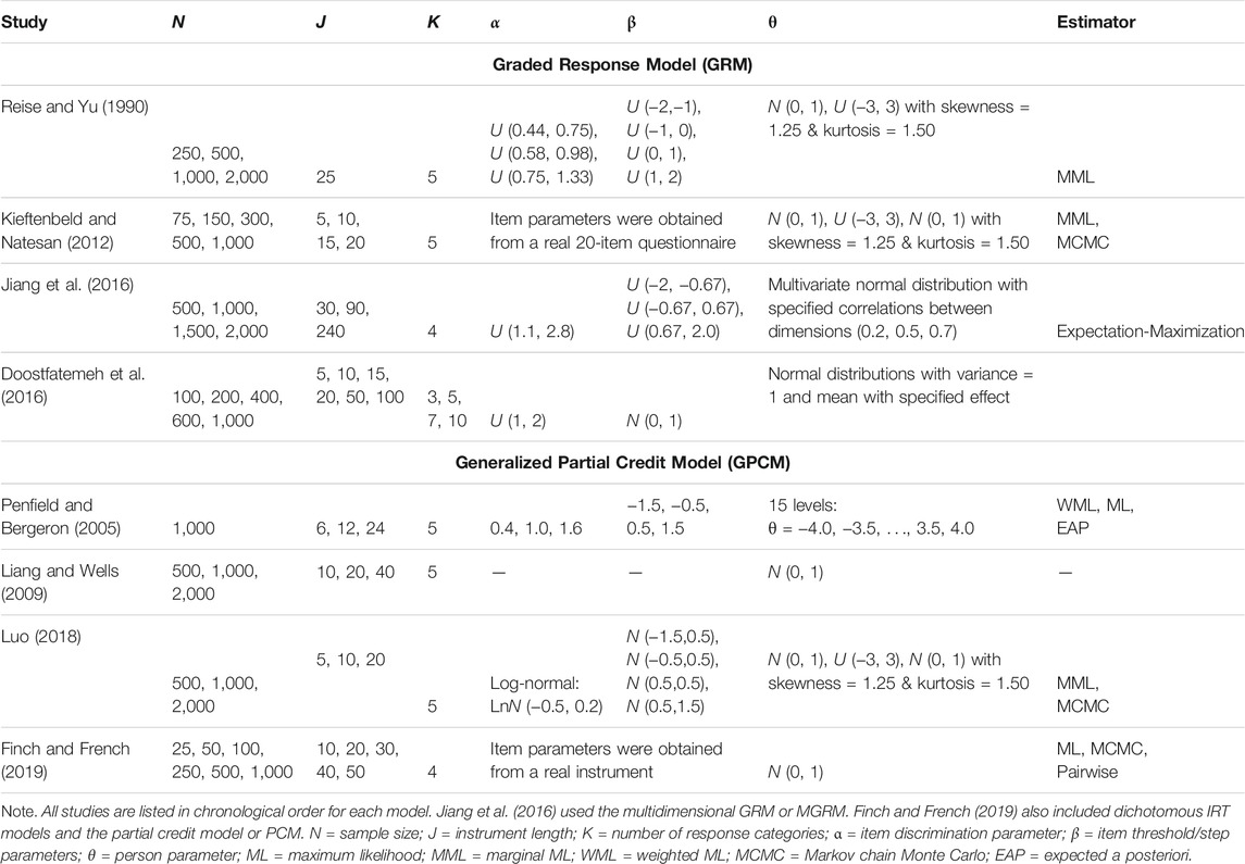
TABLE 1. Previous Literature on the Performance of GRM and GPCM.
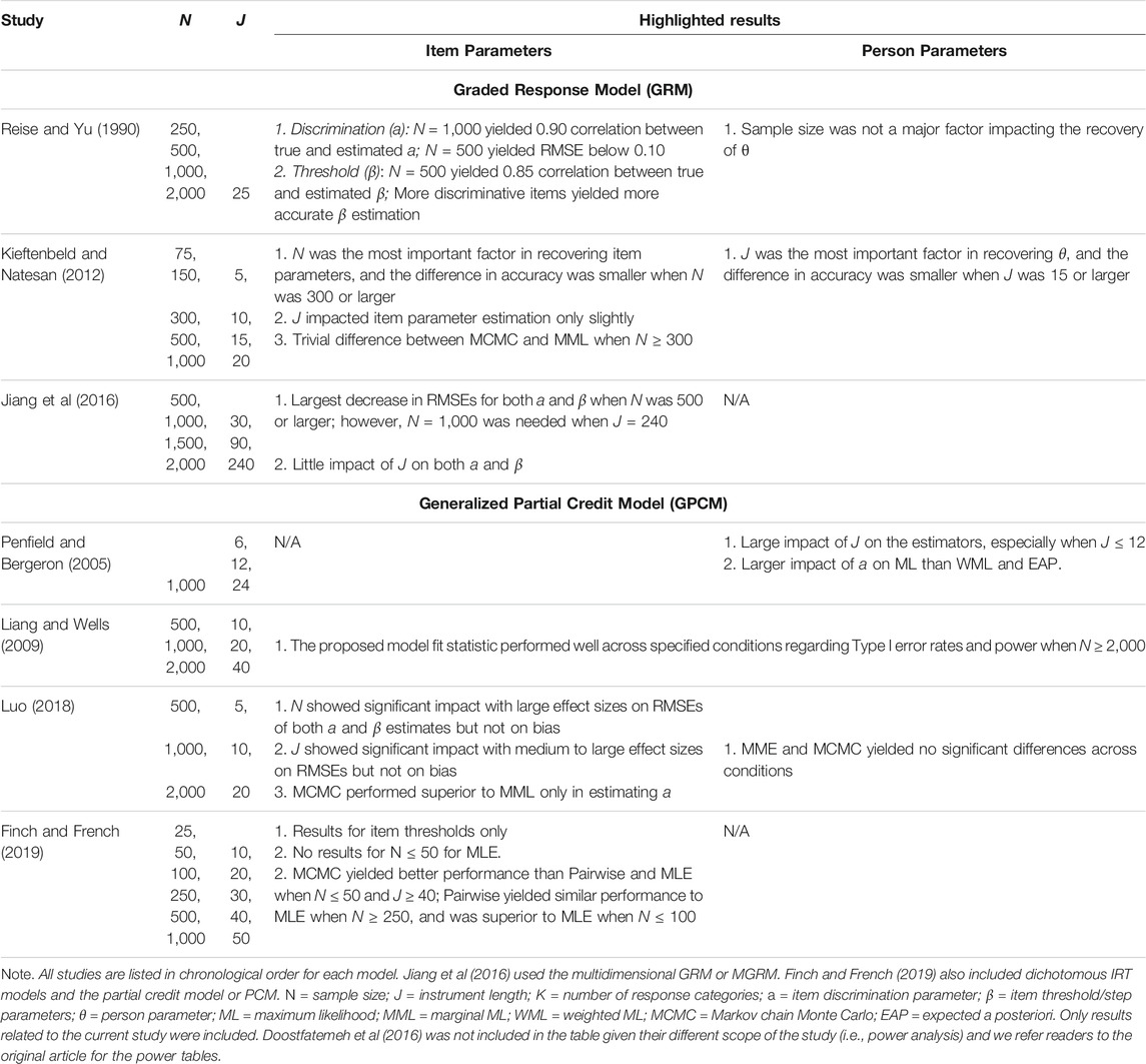
TABLE 2. Highlighted Results of Previous Literature on the Performance of GRM and GPCM Regarding Sample Size and Instrument Length.
The investigation of the performance of GRM mainly lied in Reise and Yu (1990) and Kieftenbeld and Natesan (2012). Reise and Yu (1990) examined the performance of the GRM under various conditions using an instrument consisting of 25 items with five response categories. In addition to exploring the distribution of the latent trait (or theta) and the item discrimination parameter (three discrimination levels representing poor, medium, and good item quality), the authors investigated four sample size conditions (N = 250; 500; 1,000; and 2,000). Sample size had the most pronounced effect on the correlations with larger sample sizes (i.e., 2,000) producing α = 0.95, suggesting that 1,000 examinees were needed to maintain an average true estimated α correlation of 0.90. Sample size did not appear to influence the estimation accuracy but did lead to lower average correlations in the condition of 250 examinees. The authors concluded that at least 500 examinees were needed to maintain RMSEs and respectable correlations. However, small sample sizes as low as 250 demonstrated adequate item parameter recovery for calibration samples.
In Kieftenbeld and Natesan (2012), the authors compared the effectiveness of two estimation methods, including marginal maximum likelihood (MML) and Markov chain Monte Carlo (MCMC), in recovering the item and person parameter estimates in GRM across instrument lengths (J = 5, 10, 15, and 20) and sample sizes (N = 75; 150; 300; 500; and 1,000). In the study, three levels of distributions of the person parameters were specified (a standard normal distribution with and without the interval from −3 to 3, plus a skewed normal distribution), whereas the item parameters were generated from a real 20-item questionnaire. Results of the study revealed that sample size was the most important factor in item parameter recovery whereas the instrument length did not impact the estimation of item parameters. A minimum sample size of 300–500 was suggested for the item parameters recovery accuracy. MCMC performed better than MML in the presence of small sample sizes (N = 75 and 150) but showed a comparable performance with MML with a sample size of 300 or larger. In terms of the recovery of person parameters, the results suggested a test length of at least 10 items (preferably 15) was needed.
Jiang et al. (2016) explored the impact of sample sizes on item parameter recovery for the multidimensional GRM (MGRM). In the study, the authors investigated the performance of a three-dimensional simple structure MGRM across five levels of sample sizes (N = 500; 1,000; 1,500; and 2,000) and three levels of instrument length (J = 30, 90, and 240). The intercorrelation between the dimensions was specified at 0.2, 0.5, and 0.7, respectively. Results indicated that a sample size of 500 provided accurate parameter estimates with an instrument length of 90 or shorter. When the test items increased to 240, a larger sample size of 1,000 was required for accurate parameter estimates.
Another study is a simulation-based power analysis conducted by Doostfatemeh et al. (2016), in which the authors investigated the sample size issue on GRM in analyzing patient-reported outcomes (PROs) in the context of health-related clinical trials. In the study, five levels of sample sizes (N = 100; 200; 400; 600; and 1,000), six levels of instrument lengths (J = 5, 10, 15, 20, 50, and 100), and four numbers of response categories (K = 3, 5, 7, and 10) were included in the design. Since clinical trials are usually used to evaluate the effectiveness of new medicine or treatments based on PROs, the authors also specified sample size allocation ratio across the experiment and control groups (N1: N2 = 1:1, 1:2, and 1:3) and the group effect (Cohen’s d = 0.2, 0.5, and 0.8). Additionally, the true item discrimination parameters were sampled from a uniform distribution of U (1, 2). The results revealed a large impact of instrument length, group effect, and allocation ratio on the required sample sizes. An instrument with a larger number of items would make it possible to recruit fewer participants for the analysis with prespecified effect size and power. For instance, assuming a medium effect (i.e., d = 0.5) and a desired power of 0.8, a sample size of at least 400 is necessary for an instrument with five items. This requirement of sample size could be decreased to 200 if the instrument consisted of 10 items or more, whereas sufficient power could not be ensured across conditions if the sample size was 100.
The investigation of the performance of GPCM mainly focused on estimations methods (e.g., Penfield and Bergeron, 2005; Luo, 2018; Finch and French, 2019) and evaluating model fit indices (e.g., Liang and Wells, 2009). Penfield and Bergeron (2005) compared the performance of three methods, including maximum likelihood (ML), weighted ML (WML), and expected a posteriori (EAP), in estimating the person parameters on GPCM. In the study, three levels of instrument length (J = 6, 12, and 24) were specified while the sample size was fixed at 1,000. Additionally, though three levels of item discrimination parameters (i.e., 0.4, 1.0, and 1.6) were specified, they were constrained to be equal across items of the same instrument. Results of the study suggested that the instrument length had a large impact on all three estimators while the item discrimination levels showed a larger influence on ML than the other two.
Luo (2018) examined the recovery of both item and person parameters on GPCM between the two estimation methods of MML and MCMC. In the study, three levels of sample size (N = 500; 1,000; and 2,000), instrument length (5, 10, and 20), and person parameter distribution (normal, uniform, and skewed) were specified. The results showed that the sample size affected the RMSEs significantly in the item location and discrimination parameter estimations, regardless of the test lengths and person distributions. To be more specific, a larger sample size resulted in a smaller RMSE. Other than that, test length was found to have significant effects on the RMSE in the person parameter estimation, indicating more items would lead to more accurate and stable ability estimates. When comparing the MMLE and MCMC, there only appeared to be significant differences in estimating item discrimination parameters, which was affected by the instrument length. Under skewed latent distribution, MMLE produced less biased estimates than MCMC; under both normal and uniform latent distributions, however, MCMC produced less biased estimates.
In Finch and French (2019), the authors compared the item threshold parameter estimation accuracy across three estimators, including MLE, MCMC, and the pairwise estimation, for both binary and polytomous IRT models (i.e., Rash, 2PL, PCM, and GPCM) under various levels of instrument length (J = 10, 20, 30, 40, and 50) and sample size (N = 25; 50; 100; 250; 500; and 1,000). To simulate the data with GPCM, item parameters were generated using the data from the Learning and Study Strategies Inventory. Results of the study on GPCM showed that a sample size of at least 250 was recommended for MLE. The pairwise estimation was comparable to the other methods when the sample size was 250 or larger and superior to MLE when the sample was 100 or fewer. An extremely small sample size (e.g., N = 25 or 50), however, might result in model non-convergence issues (the convergence criterion was set at 0.001 in the study) for both MLE and pairwise estimation, especially in the presence of a long instrument length (e.g., 40 or more items), under which situations the MCMC estimation method was favored.
The two simulation studies conducted by Liang and Wells (2009) evaluated the performance of a nonparametric model fit assessment (i.e., the root integrated squared error or RISE) under GPCM. In both studies, the instrument length was specified at 10, 20, and 40, while the sample size at 500; 1,000; and 2,000. Results revealed an acceptable performance (i.e., power ≥0.80) of the proposed fit assessment when the sample size was 2,000, regardless of the instrument length.
The previous literature has shed light on the implementation of polytomous IRT models across contexts. The aforementioned studies showed that the sample size is the most important factor in estimating item parameters (e.g., Kieftenbeld and Natesan, 2012). It is to be noted, however, current recommendations on sample sizes remain unclear in implementation of IRT models, especially for polytomous IRT models (Finch and French, 2019; Toland, 2014). Reise and Yu (1990) recommended a minimum sample size of 500 for GRM applications. As one of the earliest studies examining the sample size issue in polytomous IRT, their work was cited and discussed in the two popular textbooks in IRT, including Embretson and Reise (2000) and De Ayala (2013). Embretson and Reise (2000) suggested that a sufficient sample size was necessary for “reasonably small” (p.123) standard errors in parameter estimations. The definition of “reasonably small,” however, according to the authors, was arbitrary. In their illustration example, the GRM did not yield satisfactory threshold parameters for some items (J = 12) with a sample size of 350. De Ayala (2013) suggested a sample of at least 500 for GRM and GPCM (ideally N ≥ 1,200), and at least 250 for Rasch-based polytomous models (e.g., PCM), for a successful calibration with such models. More recent research (e.g., Kieftenbeld and Natesan, 2012; Finch and French, 2019) suggested that a smaller sample size, say 200 to 300, might also be feasible, especially when a robust estimation method (e.g., MCMC, Pairwise) was applied.
These simulation studies also revealed the impact of instrument length on the application of polytomous IRT models, especially for the estimation of person parameters (i.e., θ). A clear guideline for an optimal instrument length in the context does not exist, neither. Very limited support from previous research (e.g., Kieftenbeld and Natesan, 2012; Penfield & Bergeron; 2005) recommended an instrument of at least 12–15 items is adequate in recovering theta parameters, and this needed to be taken into account together with the sample size. The collective impact of sample size and instrument length on the performance of the models cannot be ignored. The decision should always be made by taking into account both factors as well as others such as the quality of the items on the instrument and vice versa. While further empirical support needs to be collected for clearer guidelines, a synthesis of the studies suggests that in general a minimum sample size of 200 is needed for adequate parameter recovery when the instrument consists of 10 or more items (e.g., Edwards, 2009; Kieftenbeld and Natesan, 2012; Reise and Yu, 1990). In the presence of a shorter instrument (e.g., J = 5), a sample size of at least 400 is necessary (Doostfatemeth, et al., 2016).
In practice, as stated previously, it is not uncommon that instruments consist of as few as three items (e.g., PISA) and/or a small sample size of less than 200 (Finch & French, 2019). The performance of the polytomous IRT models under such conditions, however, has not been fully investigated. For GRM, Kieftenbeld and Natesan (2012) was the only study we noticed that investigated the parameter estimation accuracy in the presence of small sample sizes (e.g., N = 75, 150, and 300) and short instrument length (e.g., J = 5, 10, and 15). The item parameters in the study, however, were obtained from the calibration of a real 20-item questionnaire, which might impact the generalizability of the results to instruments with a shorter length or varying item quality. For GPCM, Luo (2018) specified a short instrument length of five items but the minimal sample size used was 500. On the contrary, Finch and French (2019) took into account a broader selection of small sample sizes that ranged from 25 to 1,000. In their study, however, the instrument length was specified to be at least 10 and only the results of item thresholds were studied.
Further, no study investigated the impact of missing data in the application of the models. Missing data is a common issue with rating scale data across contexts and its presence could impact the performance of IRT models and lead to biased parameter estimates (Mislevy and Wu, 1988; Mislevy and Wu, 1996; De Ayala et al., 2001; Peng et al., 2007; Finch, 2008; Cheema, 2014). Additionally, no simulation study, to the best of our knowledge, was found that evaluated and compared the performance of GRM and GPCM.
Despite the increasing applications of the polytomous IRT models in instrument development and evaluation, further research is needed to guide the implementation of the models across sample size, instrument length, and missing data. Thus, the purpose of the current study is to inform the literature on expectations of performance under these conditions that have not been examined.
Methods
Simulation Design
To investigate the performance of both GRM and GPCM with rating scale data across conditions, we conducted a Monte Carlo simulation study. Specifications of the manipulated design factors were informed not only by previous studies (e.g., Reise and Yu, 1990; Finch and French, 2019) but also by applications of the selected IRT models across education and social science contexts (OECD, 2021).
Sample Size (N)
Four levels of sample size, N = 150; 300; 600; and 1,200, were specified to cover from relatively small to moderately large sample sizes.
Instrument Length (J)
Five levels of instrument length (i.e., number of questions), J = 3, 5, 7, 10, and 15, were investigated. Specifically, an instrument length of 3 questions was included because it has been used in practice (e.g., OECD, 2021) but has not been studied in the literature yet. Additionally, it is also the minimum requirement in the context of confirmatory factor analysis for the purpose of model identification.
Item Discrimination
Following Reise and Yu (1990), three levels of item discrimination levels were specified for both GRM and GPCM to cover items of poor, moderate, and good quality. Specifically, item discrimination values were randomly selected from a uniform distribution of U (0.44, 0.75) for poor items, U (0.58, 0.98) for moderate items, and U (0.75, 1.33) for good items.
Missing Rate (MR)
Three rates of missing data (MR = 10, 20, and 30%) were considered and they all followed the mechanism of missing at random (MAR, Little and Rubin, 1989; Finch, 2008). Results for complete data (i.e., MR = 0%) were used as the baseline for comparison.
In addition to the aforementioned design factors, other factors were fixed in the current study. Specifically, the number of categories (K) on a scale was fixed at five, a commonly used rating scale (1 = strongly disagree to 5 = strongly agree) across contexts. The four Item threshold/step parameters were randomly selected from uniform distributions of U (−2, −1), U (−1, 0), U (0, 1), and U (1, 2), while the person parameters followed a standard normal distribution. The missing data will be handled with the default method in the IRT analysis software package (i.e, the ltm package in R; Rizopoulos, 2018) used for the study, which is listwise (or casewise) deletion. A fully crossed design for the current study resulted in a total number of 960 conditions and each condition was replicated 500 times. The model convergence was observed and reported, too.
Data Generation
Using the simdat () function from the R package irtplay (Lim and Wells, 2020), complete item responses were generated under both GRM and GPCM for each of the conditions and replications. Following Dai et al. (2018) and Finch (2008), a hypothetical variable was firstly generated from N (0, 1) and used to generate missing responses of MAR of different rates. The variable was assumed to be inversely related to an individual’s probability of responding behavior. That is, the higher value on the hypothetical variable, the easier for the individual to leave blank on the item. The actual proportions of the simulated missing data were then examined to ensure accuracy in data generation.
Analyses and Outcome
The functions grm () and gpcm () with default settings from the R package ltm (Rizopoulos, 2018) were used to analyze each of the simulated data set with both GRM and GPCM. That is, each data set was analyzed by the two polytomous IRT models, respectively, regardless of its data generation model. By default, the ltm applies a marginal maximum likelihood estimation (MMLE) approach with the Broyden-Fletcher-Goldfarb-Shanno (BFGS) algorithm in fitting the model (Rizopoulos, 2018). Then the functions coef () and factor. scores () in the package were used to retrieve the item and person parameters, respectively. Explicitly, the person parameters were obtained with the Empirical Bayes (EB) method—a default setting in the function factor. scores ().
In the presence of missing data, by default, the package uses the available cases for the analysis (Rizopoulos, 2018). To achieve the purpose of the study, the outcomes of model convergence, parameter recovery, and model fit indices as well as test information were obtained and evaluated.
1) Model convergence. The average rate of model convergence across replications was collected for each condition using the binary convergence identifier as returned by the package.
2) Parameter recovery. Both the mean bias and root mean squared error (RMSE) over the 500 replications were used to evaluate the recovery of the item and person parameters across conditions. The mean bias was obtained as the average difference between the estimated and true parameters across items and replications. It was computed in a way that positive values suggested that the parameters were overestimated while negative values the opposite. Following Finch and French (2019), bias and RMSEs of the item step/threshold parameter estimates were averaged across the five categories for each condition.
3) Model fit indices. Log-Likelihood (LL), Akaike information criteria (AIC), and Bayesian information criteria (BIC), and test information statistics from the models were obtained to evaluate the model selection between the two IRT models (De Ayala, 2013; Finch & French, 2015).
At last, analyses of variance (ANOVAs) were conducted to investigate the effect of the design factors and their interactions on the outcomes. The significance level was controlled at the 0.05 level and
Results
Results of ANOVAs on the outcomes revealed significant high-order interactions across most of the conditions. Thus, given the large number of conditions in the study and to better describe and investigate the results, we present the results through profile plots with four main sections for 1) model convergence, 2) item parameter recovery, 3) person parameter recovery, and 4) model selection.
Part I: Model Convergence
Model convergence was monitored and recorded when analyzing the data. Results revealed no issues for either model when a correct model was selected to analyze the data (i.e., when the data were both generated and analyzed using the same model). Almost 100% convergence rate was achieved across all conditions of sample size, instrument length, item quality, and missing rate. Surprisingly, the same pattern was detected in conditions when the data were generated by GPCM but analyzed using GRM. Issues of model non-convergence arose, however, when the data were generated by GRM but analyzed using GPCM (see Figure 1). As can be noticed in the figure, generally, large sample sizes and longer scales (J ≥ 10) were more likely to result in model non-convergence, especially in the presence of low item discrimination power or poor item quality. Under conditions of J ≥ 10, especially when J = 15, nearly no convergence was achieved for instruments with poor or moderate items.
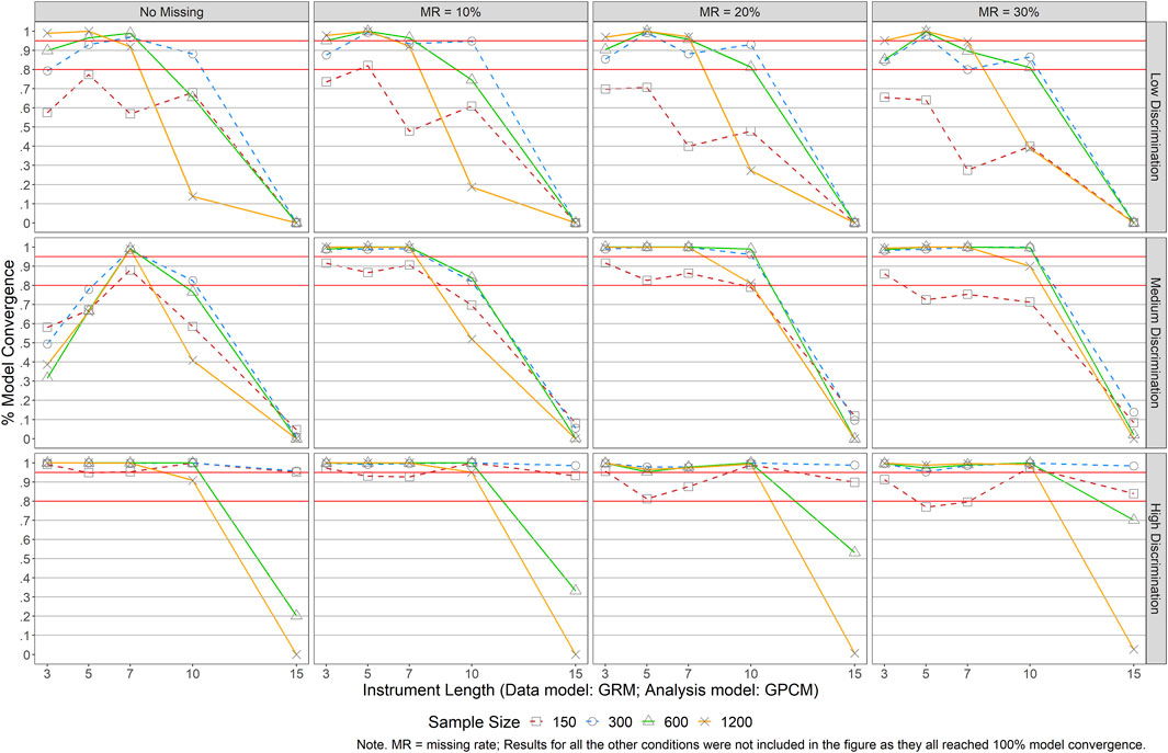
FIGURE 1. Results of Model Convergence When Data Were Generated by GRM but Analyzed with GPCM. Note. MR = missing rate; Results for all the other conditions were not included in the figure as they all reached 100% model convergence.
Part II: Recovery of Item Parameters
Figures 2, 3 present mean bias of item discriminations and thresholds for GRM (i.e., data were generated and analyzed by GRM) and GPCM (i.e., data were generated and analyzed by GPCM), respectively.1 Bias results in Figure 2 indicated a large impact of the design factors on the recovery of item discrimination parameters for GRM. Generally, when the missing rate was 10% or lower, minimal bias of the item discrimination parameters was observed across all conditions, except for the conditions of J = 3. When the missing rate was large (MR ≥ 20%), a shorter test length was associated with a larger bias in item discriminations. For example, in the MR = 20% condition, an instrument length of 7 or shorter resulted in greater bias. Regarding recovery of the item thresholds, a small bias was observed across conditions, especially when item quality was moderate or good (i.e., medium or high item discrimination levels). However, when item discrimination was low, bias in the thresholds was larger, particularly when there was a smaller sample size (i.e., <300).
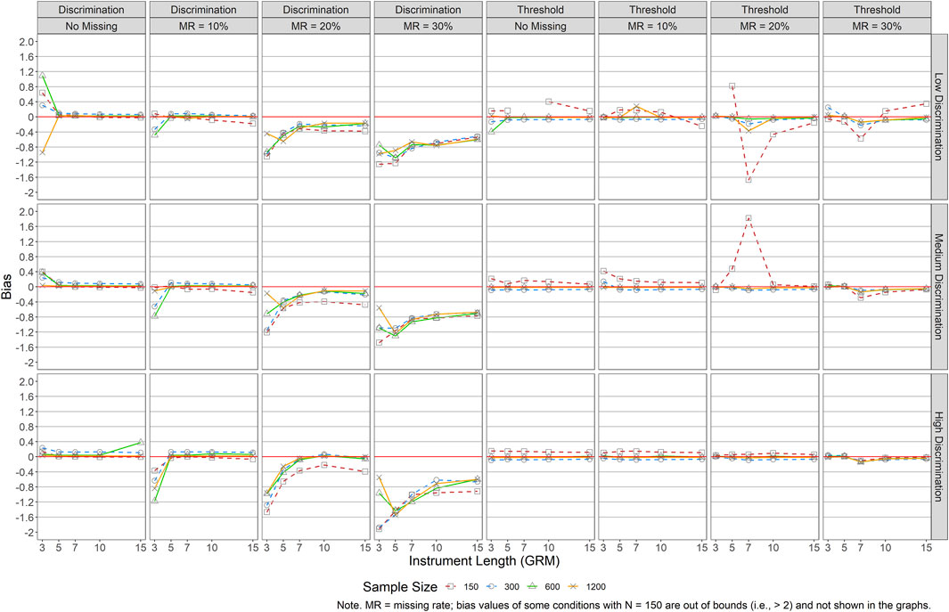
FIGURE 2. Bias of Item Parameter Estimations for GRM. Note. MR = missing rate; bias values of some conditions with N = 150 are out of bounds (i.e.,>2) and not shown in the graphs.
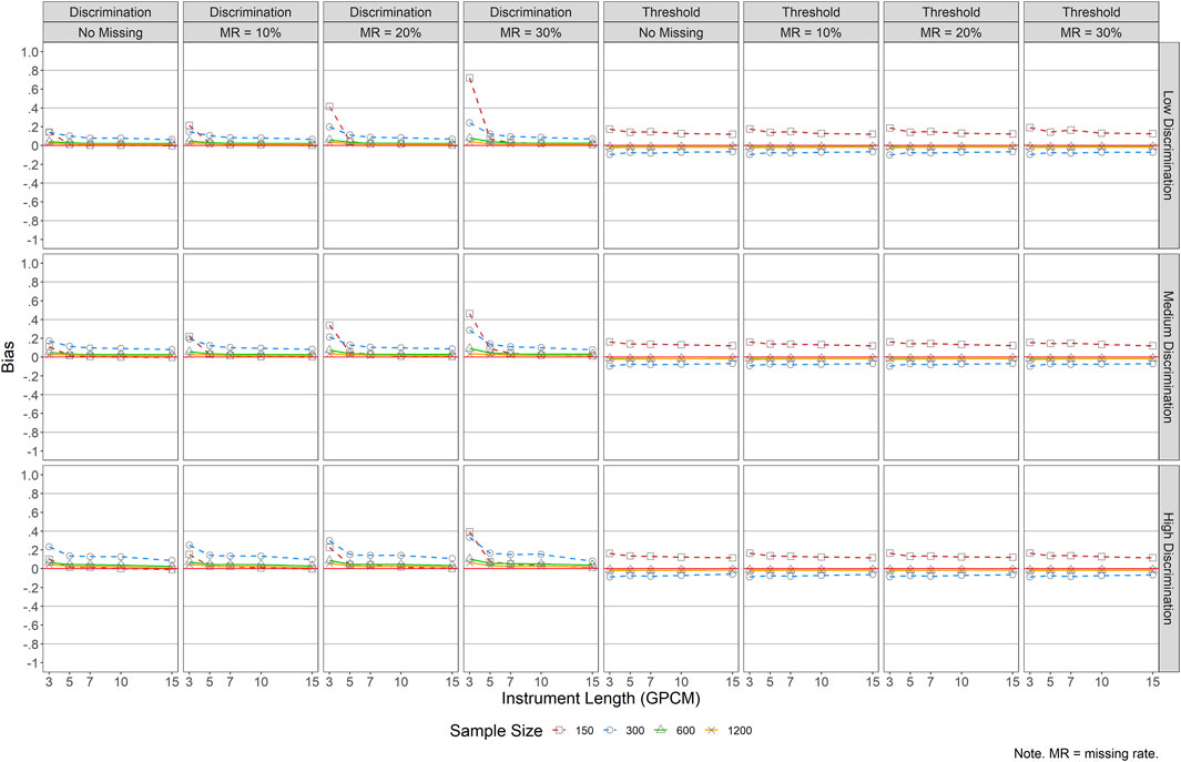
FIGURE 3. Bias of Item Parameter Estimations for GPCM. Note. MR = missing rate.
Results of GPCM in Figure 3 showed that, regardless of item quality, short instruments (J = 3) and small sample sizes (N ≤ 300) yielded relatively large bias for item discrimination parameters, especially when the missing rate was 20% or higher. Regarding item threshold estimates, bias stayed minimal across all conditions except that small sample sizes (N ≤ 300) resulted in relatively greater bias.
Figures 4, 5 present the RMSEs of the item parameters for GRM (i.e., data were generated and analyzed by GRM) and GPCM (i.e., data were generated and analyzed by GPCM), respectively. Figure 4 shows that a smaller sample size, a shorter instrument length, lower item quality, and/or a larger missing rate would result in greater RMSEs in both item discrimination and threshold estimations for GRM. Generally speaking, larger RMSEs were found across the conditions for item thresholds, especially for small sample sizes (N = 150) and large missing rates (MR = 30%). The impact of instrument length and sample size on both item parameters was small when items were of good quality (i.e., high discrimination) and there was no missing data, even in conditions with J = 3 and/or N = 150. As the missing rate increased and the item quality decreased, RMSEs increased when the instrument length was shorter and the sample size was smaller. For example, in conditions with high item quality but 10% missingness, the RMSEs increased drastically as the instrument length decreased from five items (RMSEs = 0.12–0.42 across sample sizes) to three items (RMSEs = 0.86–1.19 across sample sizes). Similarly, J ≥ 7 and N ≥ 300 were recommended when the missing data rate reached 20%, and at least J ≥ 10 and N ≥ 300 when the missing rate was 30%.
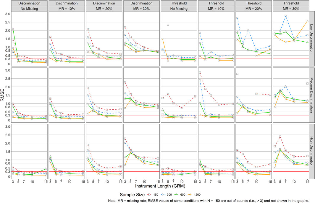
FIGURE 4. RMSE of Item Parameter Estimations for GRM. Note. MR = missing rate; RMSE values of some conditions with N = 150 are out of bounds (i.e.,>3) and not shown in the graphs.
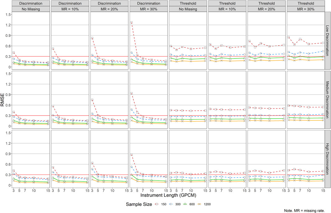
FIGURE 5. RMSE of Item Parameter Estimations for GPCM. Note. MR = missing rate.
Figure 5 reports the RMSE values for item parameter estimations under GPCM. No substantial impact of item quality was found on the RMSEs for the item discrimination parameter estimations. Other factors affected the RMSEs for the item discrimination estimation more substantially—a smaller sample size, a shorter instrument length, and a larger missing rate tended to result in higher RMSE values, especially in conditions of J = 3 and N = 150 (RMSEs = 0.51–1.27 across item quality and rates of missing data). The trend was more obvious when the missing rate was 20% or higher (RMSEs = 0.64–1.27 across item quality). For example, when J = 3, RMSEs for the discrimination parameters were always the largest across conditions, and they kept increasing as the missing rate became higher. For the estimation of item thresholds, larger sample size and higher item quality resulted in smaller RMSEs in general, and missing rates did not impact the RMSE values substantially. Regardless of instrument length, a sample size of 150 yielded the largest and constant RMSE values.
Part III: Recovery of Person Parameters
Figures 6, 7 present mean bias and RMSE results of the person parameters when a correct model was selected and used for the analyses (i.e., data were generated and analyzed by the same IRT model). Bias results in Figure 6 suggested a larger impact of the design factors on the person parameter estimations of GPCM than those of GRM, as indicated by larger absolute bias values across the graphs (e.g., lines further away from the reference line of 0). Explicitly, bias values for the GRM estimated person parameters ranged from −0.07 to 0.11 while those for the GPCM ranged from −0.27 to −0.92. Under GPCM, a longer scale tended to yield underestimated thetas with larger absolute bias values (descending lines in the graphs), which was contrary to the impact of the sample sizes, item quality, and missing data, yielding smaller absolute bias values. Under GRM, the same pattern was found across all conditions. The bias values showed nearly no impact of item quality, instrument length, and missing data on the estimation of person parameters for GRM. A small sample size (N ≤ 300) yielded larger bias values in GRM, but the magnitude (bias = −0.07–0.11) was very small compared to those generated by GPCM (bias = −0.27 ∼ −0.92).
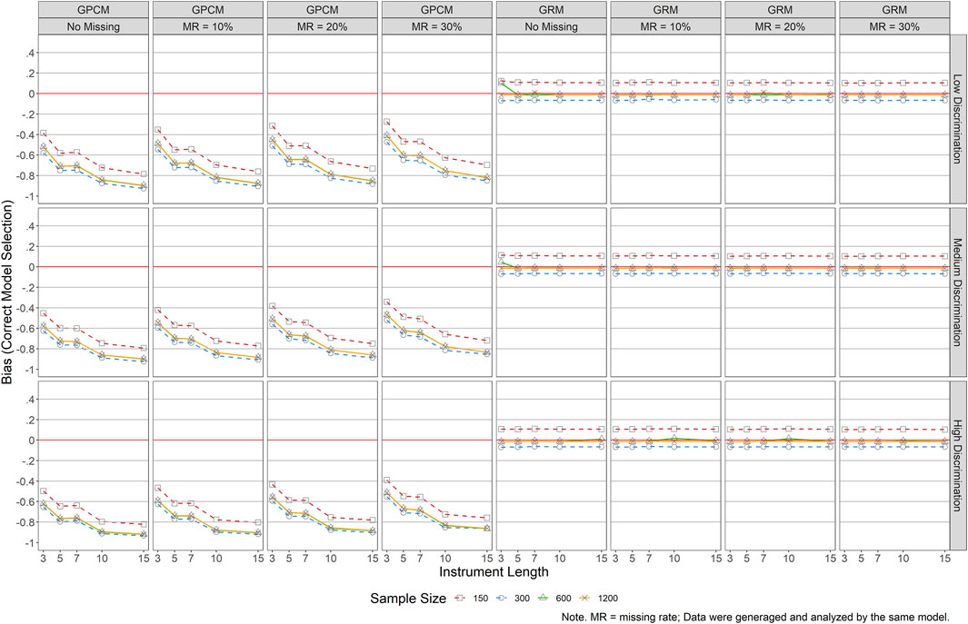
FIGURE 6. Bias Results of Person Parameter Estimations for Both GRM and GPCM (correct Model Selection). Note. MR = missing rate; Data were generaged and analyzed by the same model.
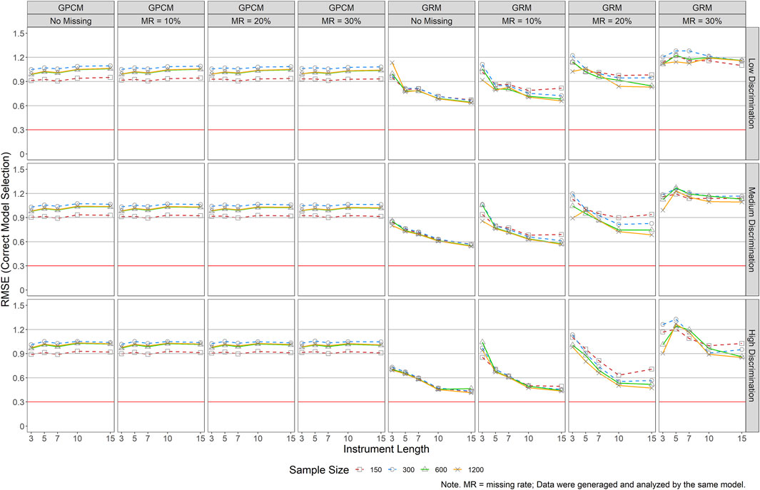
FIGURE 7. RMSE Results of Person Parameter Estimations for Both GRM and GPCM (Correct Model Selection). Note. MR = missing rate; Data were generaged and analyzed by the same model.
As indicated in Figure 7, RMSEs of GPCM revealed a constant pattern across all conditions except for the condition of N = 150, which yielded the lowest RMSEs. This was probably due to the contrary effect of instrument length (tended to yield underestimations) and other factors (tended to yield overestimations). Under GRM, greater RMSEs were noticed in the presence of a shorter scale, poorer item quality, and a larger missing rate. The impact of sample size on GRM person parameter estimations was trivial when the missing rate was 10% or less. A smaller sample size, however, tended to result in larger RMSEs when the missing rate was over 20%. RMSE results revealed a different pattern as suggested in the previous figure when comparing the two models, but what remained the same was that GRM yielded better performance in estimating the person parameters than did GPCM, as suggested by the smaller RMSEs across most of the conditions. Explicitly, RMSEs for the GRM estimated person parameters ranged from 0.44 to 1.33 while those for the GPCM ranged from0.89 to 1.40. Exceptions occurred in all the conditions with a 30% missing rate and with J ≤ 5 when the missing rate was 20%.
Figures 8, 9 display mean bias and RMSE results of person parameter estimations when an incorrect model was used for the analyses (i.e., data were generated by one model such as GRM but analyzed using a different model such as GPCM). According to the bias results in Figure 8, overall, the design factors showed no impact for GRM in estimating the person parameters for a sample size of 600 or larger when the data were generated by GPCM (the left four columns in the figure). Smaller sample sizes (N ≤ 300) yielded larger bias values, but the magnitude was small, and the pattern remained constant across all the other conditions. When GPCM was used to analyze GRM-generated data (the right four columns in the figure), the largest bias was obtained when N = 150. Meanwhile, higher discrimination (i.e., good item quality) would lead to smaller bias except when J = 3, N = 1,200 and MR = 10%, and J ≤ 7 and MR = 30%. Between the two data analysis models, GRM was related to a smaller bias and more stable performance across conditions in estimating person parameters.
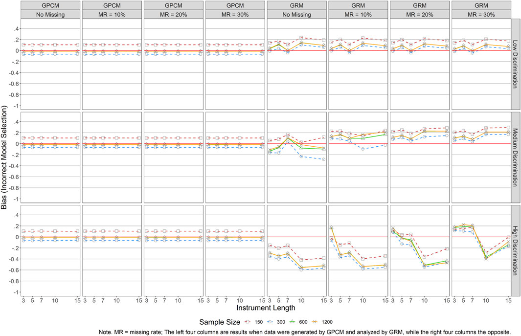
FIGURE 8. Bias Results of Person Parameter Estimations for Both GRM and GPCM (Incorrect Model Selection). Note. MR = missing rate; The left four columns are results when date were generated by GPCM and analyzed by GRM, while the right four columns the opposite.
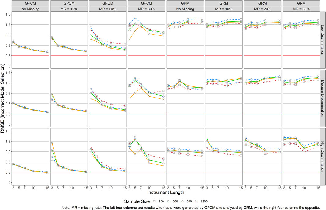
FIGURE 9. RMSE Results of Person Parameter Estimations for Both GRM and GPCM (Incorrect Model Selection). Note. MR = missing rate; The left four columns are results when date were generated by GPCM and analyzed by GRM, while the right four columns the opposite.
Figure 9 presents the RMSEs of person parameter estimations for both models in the presence of incorrect model selection. When GRM was used to analyze GPCM-generated data and when there was no missing data, longer instruments yielded smaller RMSEs while only a trivial impact was detected across levels of sample sizes and item quality. As the missing rate increased, short instruments and small sample sizes resulted in greater RMSEs. This pattern became obvious in conditions with J = 3 when MR = 10%, J ≤ 5 and N = 150 when MR = 20%, and J ≤ 7 when MR = 30%. On the other hand, when GPCM was used to analyze GRM generated data, greater RMSEs were detected across almost all conditions, especially in conditions of small sample sizes (N ≤ 300) and larger missing rates.
Part IV: Results of Model Selection
Model selection was evaluated for both models by obtaining the rate of correct model selection across conditions using AIC, BIC, LL, and test information. Specifically, a model was selected for smaller AIC and BIC values and larger LL and test information values. Figure 10 presents the results for GRM. Similar patterns were detected across AIC, BIC, and LL. In general, longer instruments and larger sample sizes yielded a higher rate of correct model selection, whereas the impact of missing data and item quality was relatively small. It became more demanding for small sample sizes (N ≤ 300) and short instruments (J ≤ 7) to reach a desired rate of 80%. For instance, when there was no missing data, the rate was above 80% across all conditions when N = 1,200. When N = 600, an instrument length of at least five items (J ≥ 5) was needed to maintain the same rate. When N = 300, at least seven items (J ≥ 7) were recommended. When N = 150, at least 10 items (J ≥ 10) were necessary. The model selection criterion of test information was more impacted by item quality than other factors except for conditions with J = 3 and N = 150. When items of an instrument were of good quality (i.e., high item discrimination), only conditions with J = 3 and N = 150 reported a correct model selection rate below 80% when MR ≥ 20%. When items were of moderate quality, a similar pattern was detected across all missing data rates. The pattern was a bit off when items were of poor quality, especially for small sample sizes and both short (J ≤ 5) and long (J = 15) instruments.
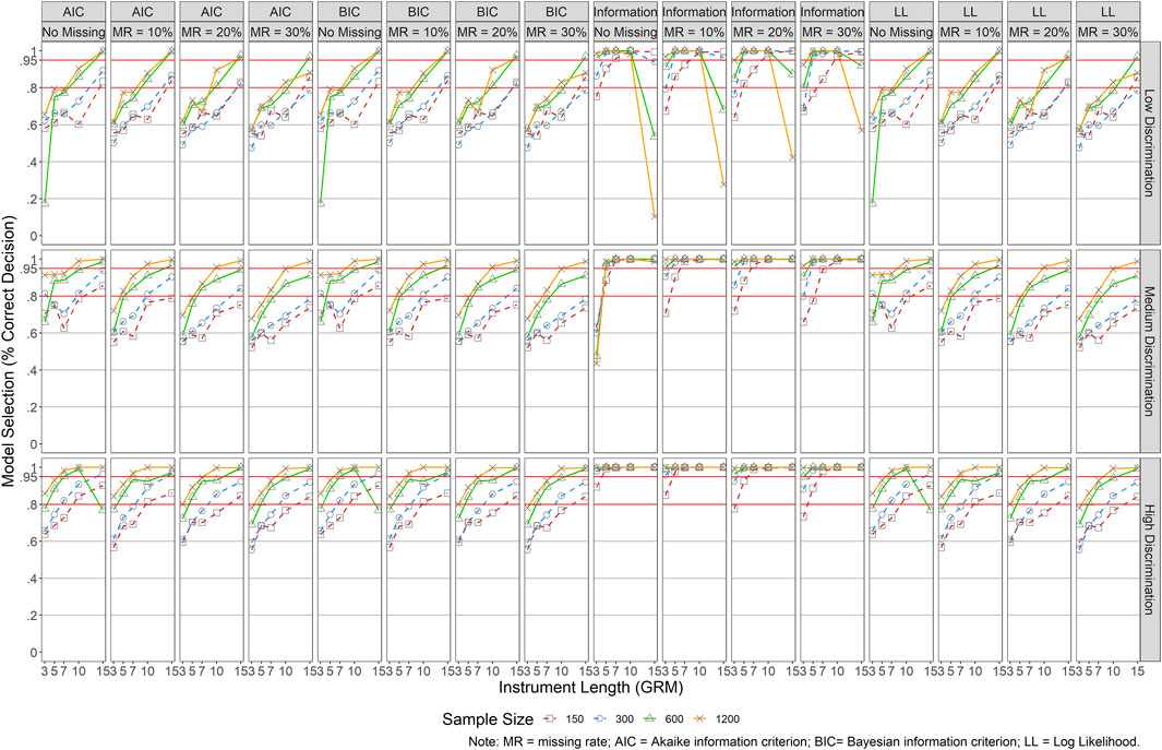
FIGURE 10. Results of Model Specification/Selection for GRM. Note. MR = missing rate; AIC = Akaike information criterion; BIC = Bayesian information criterion; LL = Log Liklihood.
Figure 11 presents the results for GPCM, and similar patterns were detected for AIC, BIC, and LL as those reported for GRM but with relatively higher rates of correct model selection in the same conditions. The largest discrepancy of results lied in those of test information, in which GPCM was rarely favored.
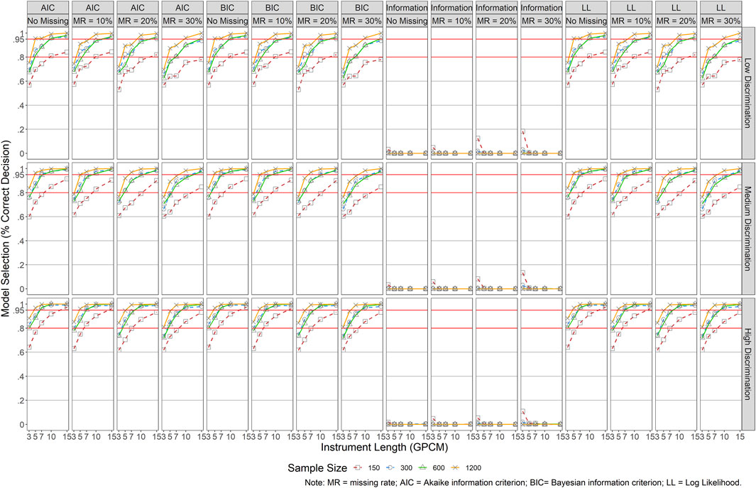
FIGURE 11. Results of Model Specification/Selection for GPCM. Note. MR = missing rate; AIC = Akaike information criterion; BIC = Bayesian information criterion; LL = Log Liklihood.
Conclusion and Discussion
The current study investigated the performance of GRM and GPCM with rating scale data across various instrument lengths, sample sizes, item quality, and missing data rates. Results from the simulation study revealed different impacts of the designed factors on the item and person parameter estimations.
Synthesizing the results of item parameter estimations for both GRM and GPCM, we identified the following patterns: 1) The estimation of item parameters for GPCM was more stable than for GRM. 2) In general, a small sample size, a short instrument length, poor item quality (i.e., lower item discrimination), and a high missing rate, tended to adversely impact the estimation accuracy of both item discrimination and threshold parameters collectively, especially for the item thresholds. 3) The item parameter estimation accuracy was lower in the presence of a short instrument (J = 3) and/or a small sample size (N = 150), especially when items were of poor quality and the missing rate was 20% or higher. 4) Generally, the impact of missing data was acceptable when MR = 10% or less. When the missing rate was high (MR ≥ 20%), a larger sample size of at least 300 and an instrument length of at least five items were required for acceptable item parameter estimations.
Regarding person parameter estimations across correct and incorrect model selections (Figures 6–9), we noticed the following patterns: 1) In general, GRM revealed more accurate theta estimates than GPCM regardless of the data generating model, as indicated by the smaller bias and RMSEs. The exception happened when there was a high rate of missing data (MR = 30%), in which GPCM yielded better performance. 2) The performance of GPCM was more stable than GRM across conditions, especially those of missing data. A large impact of missing data, especially when MR ≥ 30%, was detected on GRM in estimating person parameters. 3) Longer instrument length tended to yield more accurate person parameter estimates for GRM while it had only a small impact on those for GPCM. 4) An incorrect model selection had an adverse impact on the estimation of person parameters for both models but only with a very small size, especially for GRM.
We also investigated the impact of the selected factors on model convergence and model selection. While model convergence was not of an issue especially when a correct model was selected, model non-convergence was observed when data were generated by GRM but analyzed using GPCM, especially in the presence of small sample sizes and longer instruments. In other words, GRM seemed to be more robust than GPCM when it comes to model convergence. The use of AIC, BIC, and LL in model selection is recommended as compared to that of test information. But these indices might not be as powerful as expected in the presence of short instruments and small sample sizes (N ≤ 300), especially as the missing rate increased. The test information favored GRM across most of the conditions.
In general, the results of the study under conditions with no missing data are in line with those reported in previous studies. As stated previously, a rule of thumb from existing literature suggests a sample of 200–300 with an instrument length of 10 or more items for accurate parameter estimation. Similarly, our results support that a sample size of at least 300 in the implementation of both GRM and GPCM. An N = 150 might be feasible when the purpose is to obtain the person parameters as it will lead to inaccurate item parameter estimations and inflated type II error rates for the model fit indices.
Our results also reveal different performances of GRM and GPCM under various instrument lengths. Previous studies that showed the impact of the instrument length on the person parameters mostly lied in Kieftenbeld and Natesan (2012) work on GRM (see Table 2). Their results suggested that the difference in the accuracy of person parameter recovery was smaller when J was 15 or larger. While the maximum J in our study is 15, the results do show a notable improvement of person parameter estimations when J increases (see Figure 7). Further, based on our results, an instrument of as few as 3 items could be feasible in recovering the person parameters, especially for the GPCM. As for item parameters, J = 3 is only feasible on at least a moderate sample size (say 600). In the presence of a small sample, an instrument of at least 5 items is recommended.
Additionally, the results revealed an impact of missing data on the performance of polytomous IRT models. The impact is small when the proportion of missingness is under 10%. As the missing proportion increases, so does the requirement for a larger sample size and an instrument with more items. Although the GPCM showed a stable performance under missing data, specific approaches are still recommended to handle missingness. The application of missing data methods such as treating missing responses as incorrect, Expectation-Maximization (EM) imputation, and multiple-imputation (MI) has been studied in the context of dichotomous IRT models (e.g., De Ayalya et al., 2001; Finch, 2008; Mislevy and Wu, 1988; 1996). Their performance in the application of polytomous IRT models with rating scale data, however, remains unclear.
The present study contributes to the literature regarding our understanding of the polytomous IRT models, especially for GRM and GPCM, and their implementations. Polytomous IRT is a family of models. How to select an optimal model is often the first question for those who are tasked with IRT modeling. In practice, it is usually recommended to make the decision based on theoretical assumptions (e.g., restrictions on the item parameters), model fit, sample size (e.g., models with fewer parameters when the sample size is small), and practical concerns (e.g., useable programs; Embretson and Reise, 2000; Penfield, 2014). When it comes to the choice between GRM and GPCM, however, the issue gets complex due to the similarities of the two models such as restrictions on the parameters, which results in the same number of item parameters, and the fact that they are often equipped in the same programs (ltm, mirt, etc.). Therefore, in practice, the decision is usually made either based on the comparison of the model fit (e.g., AIC, BIC, LL, information) or arbitrarily (Edelen & Reeve, 2007).
Our results suggest that, despite the similarities of GRM and GPCM, an appropriate selection of the two models can help avoid inaccurate parameter estimations. First, in line with the literature, a model fit assessment is still recommended in general based on relative indices such as AIC and BIC. The model fit indices are less helpful, however, when the sample size is fewer than 300 and the instrument length is 5 or less. The comparison based on test information is not recommended to guide the selection of an optimal model. Second, the decision should be made in considering the factors that have different impacts on the performance of the two models, especailly for sample size, instrument length, and the presence of missing data. It is also important to note that the models performed differently with respect to the accuracy of item and person parameters. Decisions should also be made with caution in the presence of a small sample size (N = 150) and/or a short instrument length (J = 3), especially in the presence of missing data and poor item quality. When the rate of missing data is 20% or lower, GRM could be a good choice as it yields more accurate parameter estimations, especially for the person parameters. When the missing rate is over 30%, however, GPCM is recommended as its performance is relatively more stable under large missingness. Further, GRM could be an alternative in the presence of a non-convergence issue in the implementation of GPCM.
We acknowledge that the generalizations of the findings are limited to the selection of design factors in the current simulation study. As Embretson & Reise (2000, p.123) pointed out “Yet simulation studies are useful only if the data matches the simulated data.” In practice, in considering whether a polytomous IRT model should be used to analyze the rating scale data and further, which model should be selected, the decision should be always made collectively with caution by taking into account multiple factors. While our results suggest the use of GRM or GPCM when the sample size is as small as 150 under certain conditions (e.g., no missing data, high item discrimination, long instrument length), it is important to note that we used the MML estimation method to obtain the parameters. In practice, there might be situations with very small sample sizes such as 100 or 50. With such a small sample size, either of the models might not even converge and return any results with MML. For example, the GPCM did not yield results for conditions N ≤ 50 in Finch and French (2019). In the presence of such situations, other estimation methods that are more robust to small sample sizes such as MCMC or pairwise estimation might be considered. Future research should be conducted to examine the effectiveness of different estimation methods for both GRM and GPCM. Further, we only considered a rating scale with five response categories while in practice it could vary from three to many. Additionally, in the study, we assumed the missing responses to the MAR mechanism and handled the missing data with the default procedure in the software package (i.e., listwise deletion). Future studies should also take these factors such as the impact of different missing data handling approaches into account to further investigate the performance of both models across contexts.
Data Availability Statement
The raw data supporting the conclusion of this article will be made available by the authors, without undue reservation.
Author Contributions
SD developed the original idea and study design, conducted the data analyses and interpretation, performed the majority of the writing and graphing, guided the overall research process, and contributed to editing. TV, OK, HH, YX, and CD contributed to conceptualizing the study design, wrote part of the manuscript (in particular in the literature review and the results writeup), and contributed to editing. XW contributed to developing the original idea and study design, wrote the abstract, and contributed to editing.
Conflict of Interest
The authors declare that the research was conducted in the absence of any commercial or financial relationships that could be construed as a potential conflict of interest.
Publisher’s Note
All claims expressed in this article are solely those of the authors and do not necessarily represent those of their affiliated organizations, or those of the publisher, the editors and the reviewers. Any product that may be evaluated in this article, or claim that may be made by its manufacturer, is not guaranteed or endorsed by the publisher.
Acknowledgments
We gratefully thank Drs. Brian French and Dubravka Svetina Valdivia for their wonderful suggestions and edits throughout the process of this study.
Footnotes
1In this section, we only present item parameter recovery results when data were generated and analyzed by the same model. Due to the different nature of the two models (indirect vs. direct), the estimated item parameters and the true values are not comparable if a wrong model is selected to analyze the data.
References
Ayala, R. J., Plake, B. S., and Impara, J. C. (2001). The Impact of Omitted Responses on the Accuracy of Ability Estimation in Item Response Theory. J. Educ. Meas. 38 (3), 213–234. doi:10.1111/j.1745-3984.2001.tb01124.x
Burt, W., Kim, S., Davis, L. L., and Dodd, B. G. (2003). A Comparison of Item Exposure Control Procedures Using a CAT System Based on the Generalized Partial Credit Model. Chicago: Annual Meeting of the American Educational Research Association.
Carle, A. C., Jaffee, D., Vaughan, N. W., and Eder, D. (2009). Psychometric Properties of Three New National Survey of Student Engagement Based Engagement Scales: An Item Response Theory Analysis. Res. High Educ. 50 (8), 775–794. doi:10.1007/s11162-009-9141-z
Cheema, J. R. (2014). Some General Guidelines for Choosing Missing Data Handling Methods in Educational Research. J. Mod. Appl. Stat. Methods 13 (2), 3. doi:10.22237/jmasm/1414814520
Cordier, R., Munro, N., Wilkes-Gillan, S., Speyer, R., Parsons, L., and Joosten, A. (2019). Applying Item Response Theory (IRT) Modeling to an Observational Measure of Childhood Pragmatics: The Pragmatics Observational Measure-2. Front. Psychol. 10, 408. doi:10.3389/fpsyg.2019.00408
Dai, S., Svetina, D., and Chen, C. (2018). Investigation of Missing Responses in Q-Matrix Validation. Appl. Psychol. Meas. 42 (8), 660–676. doi:10.1177/0146621618762742
De Ayala, R. J. (2013). The Theory and Practice of Item Response Theory. New York, NY: Guilford Publications.
Doostfatemeh, M., Taghi Ayatollah, S. M., and Jafari, P. (2016). Power and Sample Size Calculations in Clinical Trials with Patient-Reported Outcomes under Equal and Unequal Group Sizes Based on Graded Response Model: A Simulation Study. Value Health 19 (5), 639–647. doi:10.1016/j.jval.2016.03.1857
Eichenbaum, A., Marcus, D., and French, B. F. (2019). Item Response Theory Analysis of the Psychopathic Personality Inventory-Revised. Assessment 26, 1046–1058. doi:10.1177/1073191117715729
Embretson, S. E., and Reise, S. P. (2000). Item Response Theory for Psychologists. Mahwah, NJ: Psychology Press.
Finch, H. (2008). Estimation of Item Response Theory Parameters in the Presence of Missing Data. J. Educ. Meas. 45 (3), 225–245. doi:10.1111/j.1745-3984.2008.00062.x
Finch, H., and French, B. F. (2019). A Comparison of Estimation Techniques for IRT Models with Small Samples. Appl. Meas. Edu. 32 (2), 77–96. doi:10.1080/08957347.2019.1577243
French, B. F., and Vo, T. T. (2020). Differential Item Functioning of a Truancy Assessment. J. Psychoeducational Assess. 38 (5), 642–648. doi:10.1177/0734282919863215
Fung, H. W., Chung, H. M., and Ross, C. A. (2020). Demographic and Mental Health Correlates of Childhood Emotional Abuse and Neglect in a Hong Kong Sample. Child. Abuse Negl. 99, 104288. doi:10.1016/j.chiabu.2019.104288
Glockner-Rist, A., and Hoijtink, H. (2003). The Best of Both Worlds: Factor Analysis of Dichotomous Data Using Item Response Theory and Structural Equation Modeling. Struct. Equation Model. A Multidisciplinary J. 10 (4), 544–565. doi:10.1207/s15328007sem1004_4
Gomez, R. (2008). Parent Ratings of the ADHD Items of the Disruptive Behavior Rating Scale: Analyses of Their IRT Properties Based on the Generalized Partial Credit Model. Personal. Individual Differences 45 (2), 181–186. doi:10.1016/j.paid.2008.04.001
Hagedoorn, E. I., Paans, W., Jaarsma, T., Keers, J. C., van der Schans, C. P., Luttik, M. L., et al. (2018). Translation and Psychometric Evaluation of the Dutch Families Importance in Nursing Care: Nurses' Attitudes Scale Based on the Generalized Partial Credit Model. J. Fam. Nurs. 24 (4), 538–562. doi:10.1177/1074840718810551
Jiang, S., Wang, C., and Weiss, D. J. (2016). Sample Size Requirements for Estimation of Item Parameters in the Multidimensional Graded Response Model. Front. Psychol. 7, 109. doi:10.3389/fpsyg.2016.00109
Kieftenbeld, V., and Natesan, P. (2012). Recovery of Graded Response Model Parameters. Appl. Psychol. Meas. 36 (5), 399–419. doi:10.1177/0146621612446170
Langer, M. M., Hill, C. D., Thissen, D., Burwinkle, T. M., Varni, J. W., and DeWalt, D. A. (2008). Item Response Theory Detected Differential Item Functioning between Healthy and Ill Children in Quality-Of-Life Measures. J. Clin. Epidemiol. 61 (3), 268–276. doi:10.1016/j.jclinepi.2007.05.002
Li, Y., and Baser, R. (2012). Using R and WinBUGS to Fit a Generalized Partial Credit Model for Developing and Evaluating Patient-Reported Outcomes Assessments. Stat. Med. 31 (18), 2010–2026. doi:10.1002/sim.4475
Liang, T., and Wells, C. S. (2009). A Model Fit Statistic for Generalized Partial Credit Model. Educ. Psychol. Meas. 69 (6), 913–928. doi:10.1177/0013164409332222
Lim, H., and Wells, C. S. (2020). Irtplay: Unidimensional Item Response Theory Modeling (R Package Version 1.6.2) [R package]. Available at: https://CRAN.R-project.org/package=irtplay
Little, R. J., and Rubin, D. B. (1989). The Analysis of Social Science Data with Missing Values. Sociological Methods Res. 18 (2–3), 292–326. doi:10.1177/0049124189018002004
Luo, Y. (2018). Parameter Recovery with Marginal Maximum Likelihood and Markov Chain Monte Carlo Estimation for the Generalized Partial Credit Model. ArXiv:1809.07359 [Stat]. Available at: http://arxiv.org/abs/1809.07359
Masters, G. N. (1982). A Rasch Model for Partial Credit Scoring. Psychometrika 47 (2), 149–174. doi:10.1007/bf02296272
Maydeu-Olivares, A., Cai, L., and Hernández, A. (2011). Comparing the Fit of Item Response Theory and Factor Analysis Models. Struct. Equation Model. A Multidisciplinary J. 18 (3), 333–356. doi:10.1080/10705511.2011.581993
Mislevy, R. J., and Wu, P.-K. (1988). Inferring Examinee Ability when Some Item Responses Are Missing. ETS Res. Rep. Ser. 1988 (2), i–75. doi:10.1002/j.2330-8516.1988.tb00304.x
Mislevy, R. J., and Wu, P.-K. (1996). Missing Responses and IRT Ability Estimation: Omits, Choice, Time Limits, and Adaptive Testing. ETS Res. Rep. Ser. 1996 (2), i–36. doi:10.1002/j.2333-8504.1996.tb01708.x
Muis, K. R., Winne, P. H., and Edwards, O. V. (2009). Modern Psychometrics for Assessing Achievement Goal Orientation: A Rasch Analysis. Br. J. Educ. Psychol. 79 (3), 547–576. doi:10.1348/000709908X383472
Muraki, E. (1992). A Generalized Partial Credit Model: Application of an EM Algorithm. ETS Res. Rep. Ser. 1992 (1), i–30. doi:10.1002/j.2333-8504.1992.tb01436.x
Nering, M. L., and Ostini, R. (2011). Handbook of Polytomous Item Response Theory Models. Taylor & Francis.
OECD (2021). PISA 2018 Technical Report. Paris: Organization for Economic Co-operation and Development (OECD). https://www.oecd.org/pisa/data/pisa2018technicalreport/.
Pastor, D. A., Dodd, B. G., and Chang, H.-H. (2002). A Comparison of Item Selection Techniques and Exposure Control Mechanisms in CATs Using the Generalized Partial Credit Model. Appl. Psychol. Meas. 26 (2), 147–163. doi:10.1177/01421602026002003
Penfield, R. D. (2014). An NCME Instructional Module on Polytomous Item Response Theory Models. Educ. Meas. Issues Pract. 33 (1), 36–48. doi:10.1111/emip.12023
Penfield, R. D., and Bergeron, J. M. (2005). Applying a Weighted Maximum Likelihood Latent Trait Estimator to the Generalized Partial Credit Model. Appl. Psychol. Meas. 29 (3), 218–233. doi:10.1177/0146621604270412
Peng, C.-Y. J., Harwell, M., Liou, S.-M., and Ehman, L. H. (2007). “Advances in Missing Data Methods and Implications for Educational Research,” in Real Data Analysis. Editor S. Sawilowsky (Charlotte, NC: Information Age Publishing, Inc.), 31–78.
Raju, N. S., Laffitte, L. J., and Byrne, B. M. (2002). Measurement Equivalence: A Comparison of Methods Based on Confirmatory Factor Analysis and Item Response Theory. J. Appl. Psychol. 87 (3), 517–529. doi:10.1037/0021-9010.87.3.517
Reise, S. P., and Yu, J. (1990). Parameter Recovery in the Graded Response Model Using MULTILOG. J. Educ. Meas. 27 (2), 133–144. doi:10.1111/j.1745-3984.1990.tb00738.x
Rizopoulos, D. (2018). Ltm: Latent Trait Models Under IRT (R Package Version 1.1-1) [R package]. Available at: https://CRAN.R-project.org/package=ltm
Samejima, F. (1969). Estimation of Latent Ability Using a Response Pattern of Graded Scores. Psychometr. Monogr. Suppl. 34 (4), 100.
Sharkness, J., and DeAngelo, L. (2011). Measuring Student Involvement: A Comparison of Classical Test Theory and Item Response Theory in the Construction of Scales from Student Surveys. Res. High Educ. 52 (5), 480–507. doi:10.1007/s11162-010-9202-3
Uttaro, T., and Lehman, A. (1999). Graded Response Modeling of the Quality of Life Interview. Eval. Program Plann. 22 (1), 41–52. doi:10.1016/s0149-7189(98)00039-1
Wang, S., and Wang, T. (2002). Relative Precision of Ability Estimation in Polytomous CAT: A Comparison under the Generalized Partial Credit Model and Graded Response Model.
Keywords: IRT, GRM, GPCM, sample size, instrument length, missing data
Citation: Dai S, Vo TT, Kehinde OJ, He H, Xue Y, Demir C and Wang X (2021) Performance of Polytomous IRT Models With Rating Scale Data: An Investigation Over Sample Size, Instrument Length, and Missing Data. Front. Educ. 6:721963. doi: 10.3389/feduc.2021.721963
Received: 07 June 2021; Accepted: 06 September 2021;
Published: 17 September 2021.
Edited by:
Yong Luo, Educational Testing Service, United StatesReviewed by:
Zhehan Jiang, University of Alabama, United StatesShangchao Min, Zhejiang University, China
Ting Wang, University of Missouri, United States
Copyright © 2021 Dai, Vo, Kehinde, He, Xue, Demir and Wang. This is an open-access article distributed under the terms of the Creative Commons Attribution License (CC BY). The use, distribution or reproduction in other forums is permitted, provided the original author(s) and the copyright owner(s) are credited and that the original publication in this journal is cited, in accordance with accepted academic practice. No use, distribution or reproduction is permitted which does not comply with these terms.
*Correspondence: Shenghai Dai, cy5kYWlAd3N1LmVkdQ==