Diagnosing Student Node Mastery: Impact of Varying Item Response Modeling Approaches

An important feature of learning maps, such as Dynamic Learning Maps and Enhanced Learning Maps, is their ability to accommodate nation-wide specifications of standards, such as the Common Core State Standards, within the map nodes along with relevant instruction. These features are especially useful for remedial instruction, given that accurate diagnosis is available. The year-end achievement tests are potentially useful in this regard. Unfortunately, the current use of total score or area sub-scores are neither sufficiently precise nor sufficiently reliable to diagnose mastery at the node level especially when students vary in their patterns of mastery. The current study examines varying approaches to using the year-end test for diagnosis. Prediction at the item level was obtained using parameters from varying item response theory (IRT) models. The results support using mixture class IRT models predicting mastery in which either items or node scores vary in difficulty for students in different latent classes. Not only did the mixture models fit better but trait score reliability was also maintained for the predictions of node mastery.

Introduction

Learning maps can potentially guide instruction for students if their mastery is assessed. Several learning maps or learning progressions have been developed. Cameto et al., (2012) described various types of organized learning models, including fine-grained learning maps to represent mathematical skills. Learning maps provide a visual representation of hypothesized pathways to increase the understanding of the learning targets (Hess, Kurizaki, and Holt, 2009), by representing successively more sophisticated ways of thinking about the content (Wilson and Bertenthal, 2005). For example, dynamic learning maps (DLM) and enhanced learning maps (ELM) for mathematics consist of thousands of nodes and multiple pathways that organize the knowledge, skills, and aspects of cognition related to performance.

An important feature of learning maps is to be able to accommodate nation-wide standards for the various grade levels, such as the Common Core State Standards (CCSS). CCSS in mathematics has the following five content areas: number sense, ratio and proportions, expressions and equations, geometry, and statistics and probability. Standards are nested within a content area to define very specific skills and knowledge for the grade level. For example, a seventh grade standard nested in the number sense area is “Describe situations in which opposite quantities combine to make 0” (Kansas State Department of Education, 2017, p. 58).

Both ELM and DLM were developed in a series of research projects (Kingston et al., 2016; Kingston and Broaddus, 2017) to be a superset of state standards. ELM and DLM contain networks of nodes that define prerequisite skills. Each standard for a particular state can be identified on the map as a major node (e.g., clusters of skills), along with its precursor and successor skills. Importantly, major nodes in ELM and DLM are related to instruction.

The beginning of a new school year is a particularly important time to assess student mastery of skills to determine if remedial instruction is needed. But how to determine the most appropriate instruction for individual students? As noted by Kingston and Broaddus (2017), determining relevant remedial instruction involves at least two requirements: 1) providing sufficiently precise diagnosis of skills, knowledge, and cognitive competencies of students and 2) linking the results to instruction. The first requirement involves the psychometric procedures for diagnosis while the second requirement involves linking the assessment to learning map nodes for which relevant instructional resources are available.

Providing precise diagnosis of student mastery has inspired a broad range of research and development, including formative classroom assessments. Research efforts have led to the availability of many formative tests (e.g., GMADE and Pearson, 2018) that potentially could be linked to instruction. However, since yearly accountability goals, such as CCSS, involve many standards (e.g., 15 to 20 standards are not uncommon), it would be inefficient to administer enough tests for a reliable overview of a student’s mastery of the standards that are linked to learning maps. Thus, a starting point is needed to diagnose potential areas for remedial instruction.

The assessments for state standards from the previous year are the tests that are most likely to be available to teachers as a new school year begins. The content validity of the year-end tests rests on representing the standards deemed by various educational panels to cover the current grade level skills. These skills are viewed as essential for the next grade level, as students falling below a certain overall score level may not be promoted. Thus, diagnostic information from the year-end test is important at the beginning to the school year to uncover “prerequisite” areas without mastery. The available overall test scores are deemed reliable for diagnosing students’ overall mastery of the various measured standards. When based on item response theory (IRT), items for the standards can be placed on a scale of relative difficulty. Overall test scores can be aligned with the scale, thus indicating relative probability of solving specific items for the standards; hence, a common scale alignment of scores and items has direct implications for mastery of specific skills. The NAEP mathematics skills maps (Nations Report Card, 2019) are an example of such alignment.

But can the year-end test results be used to determine relevant instruction for individual students? Unfortunately, diagnosis based on overall test scores can be problematic (Popham et al., 2014). A major issue is that the overall scores may not be sufficiently precise to diagnose which standards a particular student has mastered. That is, different instructional backgrounds, different test-taking strategies, and other factors can impact the relative item difficulties within and across nodes. If students have varying patterns of skill competencies, diagnosis of specific skill mastery based on total test scores is misleading.

Various psychometric approaches have been applied to year-end tests to increase diagnostic relevancy. For example, sub-scores for major areas within the CCSS are sometimes reported with overall test scores to diagnose mastery. Standards are typically clustered into global content areas, and sub-scores on the items within the areas are computed for each student. Because sub-scores are based on fewer items than overall scores, they are less reliable. But worse, they are still not sufficiently precise. That is, instruction based on learning maps is relevant to more specific standards within the area. However, sub-scores based on items representing each standard, although more specific, would be based on too few items to have sufficient reliability to diagnose mastery.

Alternatively, cognitive diagnostic models (Rupp et al., 2010) sometimes have been applied to assess patterns of competency (Li, 2011) and longitudinal growth (Pan et al., 2020). However, the number of different attributes for a cognitive diagnostic model cannot be large, as the number of possible patterns increases exponentially with the number of attributes. Thus, diagnosis is not sufficiently reliable for typical achievement tests representing 15 to 20 standards.

The current study takes a somewhat different approach. Rather than using area or node-specific sub-scores or attribute patterns, diagnosis is based on item-specific predictions using item response theory (IRT) estimated person and item parameters on a year-end test.

Several psychometric models will be compared for overall fit and diagnosis of mastery, including models that can accommodate different patterns of mastery. For the traditional binary-scored items, parameters for unidimensional, multidimensional, and mixture class IRT models will be estimated. The multidimensional and mixture class models can accommodate students’ varying patterns of item responses. Also, two polytomous IRT models will be applied to node-scored “items” from the overall test. That is, each polytomous item response represents the number of node-specific items passed by an examinee. Thus, the number of items is the number of nodes represented on the test. The two polytomous IRT models are the unidimensional partial credit model and the partial credit mixture class model.

A year-end test for middle school mathematics will be used for model comparisons. For this test, the blueprint categories are linked to CCSS-based nodes on ELM for which instruction is available. For each IRT model, mastery of the nodes will be predicted for each student based on the model parameter estimates. The models will be compared for fit, trait level reliability, and differential diagnosis of node mastery. It is hypothesized that the mixture class models will not only fit substantially better but also maintain examinee score reliability. Differential diagnosis of mastery versus non-mastery of the nodes for students is also expected from the models, with improved diagnostic accuracy resulting from using better-fitting models.

Item Response Theory–Based Approaches

In this section, the various IRT approaches are elaborated. Details on the models and implications for node prediction are reviewed. For all models, predicted node mastery for individual students involves comparing node predictions to a specified mastery cutline.

Predictions Based on Item Accuracy

For the item accuracy data, mastery assessments will be based on the mean predicted probability that an examinee solves items in a particular node. Mastery will be determined by comparing these probabilities to a predetermined cutline for mastery (e.g., probability of 0.70 or higher). For the unidimensional IRT model, both the estimated mean difficulty for items within a node (${\beta }_k^{-}$) and examinee overall trait level (${\theta }_j$) can be used to compute the probability that examinee j solves items in node k, $P\left(X_{jk}=1\right)$as follows:

$P\left(X_{jk}=1\right)= e^{{\theta }_j- {\beta }_k^{-}}/\left(1+e^{{\theta }_j-{\beta }_k^{-}}\right),(1)$

with an IRT Rasch model. In this case, the examinee’s trait level is based on all the test items and is the most reliable trait estimate.

If examinees at the same overall trait levels have varying patterns of area difficulties, however, then separate trait levels to represent each area could be more appropriate. In this case, a confirmatory multidimensional model, with specified trait areas, would be expected to fit significantly better than the unidimensional model. Thus, the trait level used to compute the probabilities for nodes in area d for examinee j, ${\theta }_{jd}$would be given as follows:

$P\left(X_{jk}=1\right)= e^{{\theta }_{jd}- {\beta }_k^{-}}/\left(1+e^{{\theta }_{jd}-{\beta }_k^{-}}\right).(2)$

However, the pattern of item responses may vary further between examinees than permitted in calibrations of probabilities in Eq. 2. That is, the varying patterns of item difficulties may lead to latent classes of examinees. In this case, a mixture distribution IRT model (e.g., Rost and von Davier, 1995) is needed. Thus, the probability that examinee j solves an item in node k depends the mean difficulty of the node in class m, ${\beta }_{km}^{-}$, and the examinee’s trait level based on class difficulties, ${\theta }_{jm}$, as follows:

$P\left(X_{jkm}=1\right)={\prod }_m{\eta }_{mj} (e^{{\theta }_{jm}-{\beta }_{km}^{-}}/\left(1+e^{{\theta }_{jm}-{\beta }_{km}^{-}}\right)),(3)$

where ${\eta }_{mj}$ is the probability that examinee j belong to class m.

Latent classes may reflect pattern differences between examinees for the various areas, similar to the multidimensional IRT models in Eq. 2. However, the classes also could reflect node differences within areas or even specific item difficulty differences within the nodes when based on item accuracy data.

Predictions Based on Node Scores

Another approach is to treat the nodes as polytomous items. That is, if the items are classified into 18 different nodes, they become 18 polytomous items in which accuracy scores are obtained for each node. Thus, if s_n is the number of score categories in node n, the probability that examine j obtains score x in node n is denoted as $P\left(X_{jnx}\right),$ where x = 0,…,s_n. The partial credit Rasch is given as follows:

$P\left(X_{jnx}\right)= \frac{e^{{\Sigma }_{k=0}^x\left({\theta }_j- {\beta }_n+ {\tau }_{nk}\right)}}{{\Sigma }_{y=0}^{s_n}{e}^{{\Sigma }_{k=0}^x\left({\theta }_j- {\beta }_n+ {\tau }_{nk}\right)}},(4)$

where${\beta }_n$ is the difficulty location of node n, ${\tau }_{nmk}$ is the threshold parameter for category k in node n, and${\theta }_j$ is examinee j’s trait level based on node scores and corresponding parameters.

The partial credit Rasch model also can be estimated as mixture class model in which the pattern of node difficulties varies across classes. In this case, the probability that examine j obtains score x in node n is denoted as $P\left(X_{jnx}\right),$ is given as follows for the mixture partial credit Rasch model:

$P\left(X_{jnx}\right)={\prod }_m{\eta }_{mj} \left[\frac{e^{{\Sigma }_{k=0}^x\left({\theta }_{jm}- {\beta }_{nm}+ {\tau }_{nkm}\right)}}{{\Sigma }_{y=0}^{s_n}{e}^{{\Sigma }_{k=0}^x\left({\theta }_{jm}- {\beta }_{nm}+ {\tau }_{nkm}\right)}}\right] ,(5)$

where ${\eta }_{mj}$ is the probability that examinee j belongs to class m, ${\beta }_{nm}$ is the difficulty location of node n in class m, ${\tau }_{nmk}$ is the parameter for category k in node n, and${\theta }_{jm}$ is examinee j’s trait level based on node difficulties in class m.

Method

Examinees

The examinees were 8,585 students in Grade 7. These students took the same form of the state mathematics achievement test in late spring.

Test

The test was the state accountability test for mathematics achievement consisting of 70 multiple choice items. The items represented blueprint categories for the major areas of mathematics for Grade 7. The items were linked to ELM node clusters that represented the various subareas in CCSS. Thus, items were linked to nodes within specific subareas for five major CCSS categories; 1) number sense (NS), 2) ratio and proportions (RP), 3) expressions and equations (EE), 4) geometry (G), and 5) statistics and probability (SP). A total of 66 items could be linked to ELM with a rater reliability of 0.876. The total number of nodes represented by the test within the areas was 18. For all subsequent statistics and analyses for the areas, number sense was combined with ratios and proportions so that the number of items per area was not less than 10. Table 1 shows the number of nodes per area and the number of items within each node.

TABLE 1

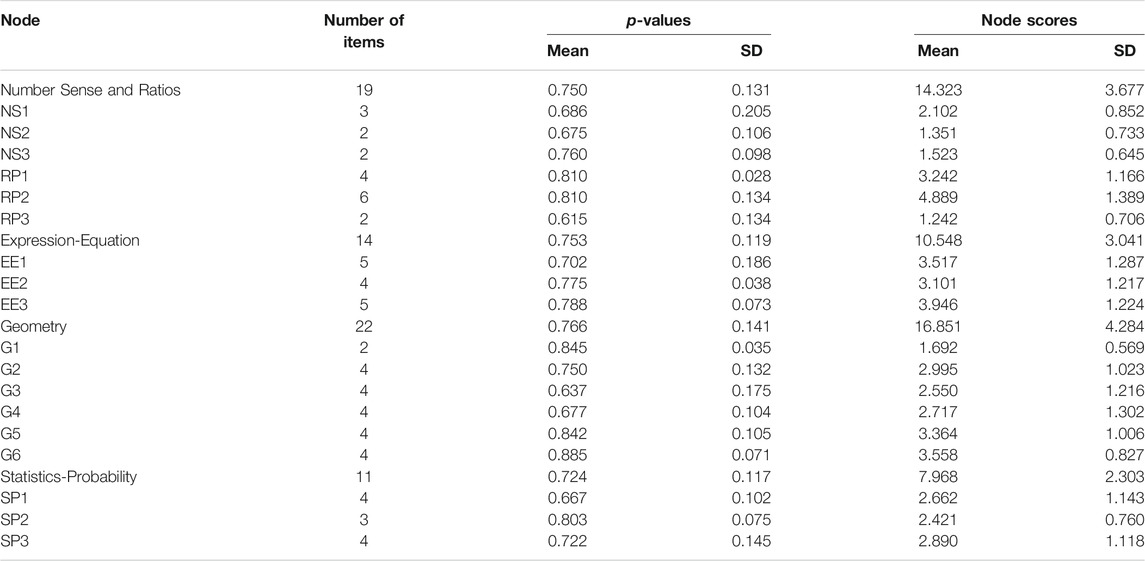
TABLE 1. Mean and standard deviations for p-values for items within the areas and nodes from binary item accuracy data.

Procedures

Five different IRT models were estimated. All models were variants of Rasch models to assure appropriate comparisons to the mixture class models.

Models based on item accuracy. Three models based on item accuracy were estimated: 1) a unidimensional Rasch model to provide a single trait level, 2) a multidimensional Rasch model consisting of independent trait level estimates for the major CCSS areas, and 3) a mixture Rasch model. For these three models, difficulties for each item were estimated using conditional maximum likelihood followed by maximum likelihood trait levels estimates based on the individual item parameters. For the multidimensional model, the dimensions correspond to areas for the standards; thus, each trait level was estimated using only items within an area. For the mixture Rasch model, the number of classes used for these estimates depended on fit and class sizes. Then, the mean estimated item difficulty was computed for each node in the three models. Performance levels for each examine on the 18 CCSS nodes was assessed using IRT parameter-based predictions as shown in Eqs 1–3. That is, the probability of passing the average item within each node was computed for each examinee, $P\left(X_{jk}=1\right)$, using the mean item difficulty for node k. For the mixture Rasch model, the parameters used depended on the latent class for which examinee j had the highest probability of belonging, as shown in Eq. 3.

Models based on node scores. Polytomous items were created for the test by scoring items for the same node into “testlets” (Thissen, Steinberg and Mooney, 1989). That is, accuracy responses on items measuring the same node were summed, thus creating 18 polytomous items.

Two models based on the node scores, the partial credit Rasch model and the mixture partial credit Rasch model, were estimated in a similar fashion as the binary item models. In the partial credit models, node scores are treated as polytomous items with multiple thresholds. Estimates for location (i.e., mean node threshold difficulty) and score category thresholds were obtained for each node. The parameters for the partial credit model were estimated as shown in Eq. 4. For the mixture partial credit Rasch model, the number of classes used for these estimates depended on fit and class sizes. Parameters were estimated as shown in Eq. 5. No additional computations were needed, as node parameters are directly estimated.

Results

A significant issue for the data is whether or not the year-end test indicates non-mastery, thus indicating a need for remedial instruction. The percentage of the 66 items solved by each student is shown on a histogram on Figure 1. A cutline of 70% correct is often used as a mastery cutline. Although many students have very high percentage passed scores, it can be seen that a substantial proportion of the students (actually, 33.7%) fall below a cutline of 0.70 for mastery. Higher mastery cutlines (e.g., 0.80) would have large numbers of students falling below it. Determining potential areas for instruction is especially important for students whose predicted scores fall below the cutline. However, even students with total proportion of items passed at 0.70 or above may have one or more areas of non-mastery.

FIGURE 1

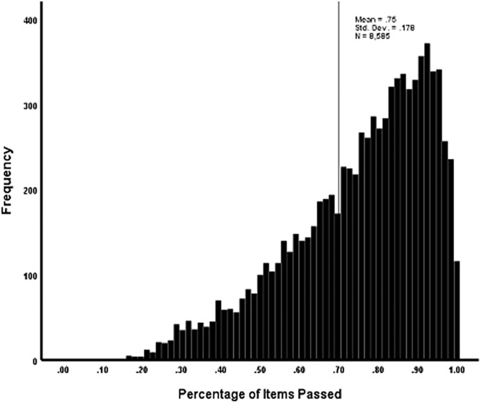
FIGURE 1. Distribution of students by percentage of test items passed.

Models Based on Item Accuracy

Descriptive statistics.Table 1 shows the means and standard deviations of the proportion of students passing the various items (p-values) by overall area and by the nodes that represent the standards. It can be seen that the mean p-values are very similar across areas and above 0.70. Thus, an overall diagnosis of relative weaknesses by area is not supported.

For nodes, Table 1 shows that the mean p-values of items in the various nodes varies more substantially. That is, the mean p-values of the items in the nodes range from 0.615 (RP3) to 0.885 (G6), indicating differences in relative mastery. That is, most students are responding correctly to the four items in G6, but many students are not responding correctly to items in RP3. Table 1 shows similar findings within areas. Thus, differential focus on the nodes, rather than areas, for possible remedial instruction is supported.

Model estimates. Some variability in the estimation software used for the various models was necessary. That is, different software was needed to estimate multidimensional and mixture class models as noted below. To assure similarity, those models (i.e., unidimensional models) that could be estimated by both programs were compared and the parameter estimates were virtually identical.

Item and person parameters were estimated for the three different IRT models. The unidimensional and multidimensional Rasch model was estimated in IRTPRO (Thissen et al., 1989) using marginal maximum likelihood. The mixture class IRT model was estimated with winMIRA (Rost and von Davier, 1995) using conditional maximum likelihood. In winMIRA, additional classes are based on person fit statistics. Fit is determined by the likelihood of a persons’ responses given the persons’ estimated trait level and item difficulty parameters. Misfitting persons are placed in a new class in which different item parameters are estimated and fit is reassessed.

Unidimensional estimates. First, the unidimensional Rasch model parameters were estimated to represent a method often used for analyzing year-end test results. As typical with Rasch models, the mean item difficulty was set to zero to identify the model. Using estimated difficulty parameters for the 66 items, person trait levels were estimated using the expected a posteriori (EAP) method. The obtained estimates (Mn = 1.552; SD = 1.274), when combined with item difficulties having a mean of zero, yields predicted percentages of items passed at the levels seen on Figure 1. Further, since total score is a sufficient statistic for person estimates with the Rasch model, the trait distribution shape would be similar that shown on Figure 1.

Multiple dimension estimates. Second, a multidimensional Rasch model was fit to the data with the four areas defining the dimensions. Thus, each item loaded on only one dimension. Model fit was significantly better than fit for the unidimensional Rasch model (Δχ²/df = 63.07; df = 9, p <0 .001). Thus, area-specific calibrations led to an overall better-fitting model.

Sub-scores for trait level were estimated separately by EAP using the Rasch model item parameters for the areas. It can be seen in Table 2 that although the estimated trait levels for the areas have strong correlations with total trait level, it is not quite as high as would be expected if the test was fully unidimensional. Further, the area intercorrelations of trait levels (0.60 and 0.70 s) were more moderate. Table 2 also shows differences in empirical reliabilities between areas and overall scores, which is related to the number of items. Reliabilities were computed with the IRT-based estimates as follows: $r_{tt}= {\sigma }_{\theta }^2/({\sigma }_{SE}^2+{\sigma }_{\theta }^2)$, where ${\sigma }_{\theta }^2$ is the variance in trait level scores and ${\sigma }_{SE}^2$ is the average standard error variance of trait level scores.

TABLE 2

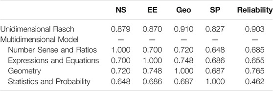
TABLE 2. Empirical reliabilities and trait level correlations for unidimensional and multidimensional Rasch models based on item accuracy data.

Although the trait level estimates using unidimensional Rasch model had a high reliability, the area-specific reliabilities are not strong, as expected. Thus, although multidimensionality was supported overall, score reliability decreased substantially.

Class-specific estimates. Mixture distribution Rasch models were also fit to the data. A series of models were estimated to determine the number of distinct latent classes. The single-class solution is the unidimensional Rasch model, as described above. With large sample sizes as in the current study (N = 8,585), the statistically significant changes with increased numbers of classes can lead to many small, but practically insignificant classes. Thus, additional class solutions were estimated until either fit was not significantly improved or the percentage of the sample in one or more classes was small (i.e., below 10%). Table 3 shows increasing fit as indicated by the significant change in χ2 up to four classes. The final four-class solution fit significantly better than the single-class solution (Δχ2/df = 53.58, p <0 .001). Person fit, as indicated by a person’s highest class probability (i.e., ${\eta }_{mj}$ in Eq. 5 above), had a mean of 0.884, supporting strong fit.

TABLE 3

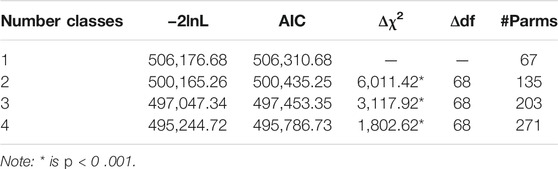
TABLE 3. Log likelihoods and fit indices for the mixture Rasch model from item accuracy data.

Table 4 presents the intercorrelations of item difficulties between the four classes and with the overall item difficulties from a single-class Rasch model. Item difficulties were estimated separately using maximum likelihood for each class using a fixed mean of 0.000 for model identification. It can be seen that the difficulties of the 66 items are only moderately correlated between classes (0.394 ≤ r ≤ 0.677). Further, the class item difficulties also vary significantly in their correlations with Rasch model item difficulties estimated from the single-class model (0.632 ≤ r ≤ 0.913).

TABLE 4

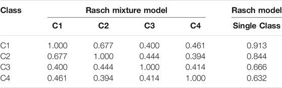
TABLE 4. Item difficulty correlations for the four latent classes from item accuracy data.

Table 5 presents descriptive statistics on trait level estimates by class. Class 1 contains more than 50% of the examinees, and the remaining examinees are split between the other three classes. In each class, the mean item difficulty is set to zero for model identification. Trait levels were estimated using the within class item difficulties for examinees within the class. The trait level empirical reliabilities were moderately high for all classes. Further, based on all examinees, trait levels estimated using the appropriate within class parameters correlated 0.999 with estimates based on a single class. However, the mean trait levels of examinees in the classes varies substantially, which has implications for item-solving probabilities. Examinees within Class 1 have the highest mean trait level. When calculated with mean item difficulty (i.e., 0 in each class), examinees in Class 1 have a predicted mean item-solving probability of 0.933. The trait level mean for examinees in Class 3 is the lowest and leads to a predicted mean item-solving probability of 0.519.

TABLE 5

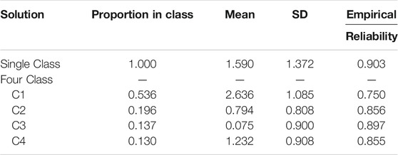
TABLE 5. Trait level means, standard deviations, and empirical reliabilities in the unidimensional and four latent-class solution from item accuracy data.

Although the mean item difficulty within each class is fixed to 0.000, as standard for identifying Rasch models, the relative difficulties for the various CCSS areas and nodes can vary within classes. Figure 2 presents the item difficulty means within the four classes and also for a single class. The areas differ substantially in relative difficulty across classes. For Class 1, the most difficult items are in the statistics and probability area, but the next most difficult items are in number sense and ratios. For Class 2, the number sense and ratio items are the easiest. Similar differences can be seen for the other classes. Thus, the relative difficulty of items in the four areas varies across classes.

FIGURE 2

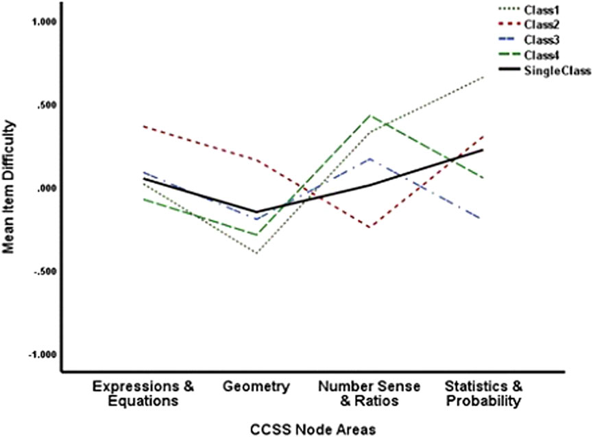
FIGURE 2. Mean item difficulty by area by class for item accuracy data.

Figure 3 presents the mean item difficulties at the CCSS node level. Similar patterns of CCSS node differences within areas are observed for some areas but not for others. For example, the greatest difference between classes is for the nodes associated with ratios and proportions. That is, the RP2 node is much easier for Class 2, but relatively harder for Class 3. Similarly, the RP1 node is much harder for Class 4 than the other classes. Thus, area differences between classes in Figure 2 do not fully describe node differences within areas.

FIGURE 3

FIGURE 3. Mean item difficulty for nodes by class for item accuracy data.

Differential diagnosis. With multiple dimensions and multiple classes leading to different results on the relative difficulty for the areas and nodes, what is the impact on diagnosing mastery for individual students? To understand mastery, it is necessary to specific a cutline. A typical cutline for mastery is that the proportion of items solved in the area equals or exceeds 0.70. The three IRT models, unidimensional, multidimensional, and mixture models, were used to predict the probability for each student that items would be solved in each of the CCSS node categories. If the probability equaled or exceeded 0.70, the student was deemed to have mastery. Probabilities below 0.70 define non-mastery.

Figure 4 presents the proportion of students in the sample for whom their predicted probabilities of solving items equals or exceeds the cutline of 0.70 by model and node. The horizontal line shows the 66.3% of students exceeding the cutline based on the overall test score as in Figure 1. It can be seen that the nodes within areas vary substantially in the predicted proportion of students who exceed the mastery cutline. For example, CCSS geometry node G3 has a much lower proportion of students with mastery than do the other five geometry nodes. Similar differences are shown in the other areas. However, the predicted sample proportions for the nodes are quite similar across the three models. These results seemingly suggest that which model is applied does not make a difference in diagnosing mastery.

FIGURE 4

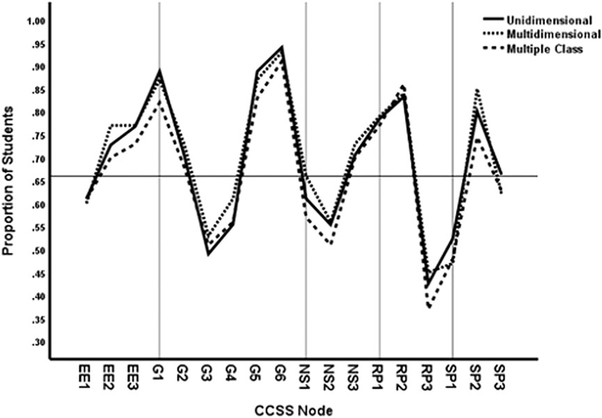
FIGURE 4. Proportion of students with mastery based on cutline 0.70 by method and CCSS node for item accuracy data.

However, although the data in Figure 4 show that the same overall percentages of students are diagnosed with mastery from the three models, we should not assume that the models diagnose the same students. Figure 5 presents the proportion of the sample with differential diagnosis by the models. As for the data in Figure 4, the three models predicted the probability that items would be solved in the various nodes for each student and compared the predictions to a cutline of 0.70 to determine mastery. Then a crosstabulation of the mastery predictions for students from pairs of models was calculated: multiple versus single trait levels and multiple versus single class diagnosis. A case was counted as differential diagnosis with respect to the single-class/trait model if either 1. masters were non-masters or 2. non-masters were masters in the comparison model.

FIGURE 5

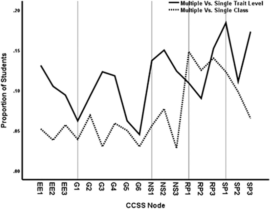
FIGURE 5. Proportion of students with differential diagnosis by method and CCSS node at cutline 0.70 for item accuracy data.

It can be seen in Figure 5 that the mastery diagnosis differs by about 5% from the multiple versus single-class comparisons for expressions and equations, geometry and number sense nodes. The ratio and proportions and statistics and probability nodes, however, differ more substantially in diagnosis from multiple versus single classes. More substantial differences in mastery diagnosis were observed using multiple versus single traits, which may reflect in part the decreased reliability of the multidimensional trait level estimates (see Table 2). The minimum difference is 5%, but most nodes are much higher. Thus, which students are diagnosed with mastery versus non-mastery of specific nodes depends on the IRT model that used for the prediction. Some differences are observed for multiple versus single classes, but multidimensional assessments based on node area lead to stronger differences.

Which students are differentially diagnosed by the varying IRT models? Person fit indices from the unidimensional and single-class solution were correlated with differential diagnosis for both multiple traits and multiple classes. For differential diagnosis from predictions based on multiple versus unidimensional traits, the correlations varied across nodes (0.060 < r < 0.428), with a mean correlation of r = 0.090. The correlations also varied across nodes for multiple versus single class differential diagnosis (0.113 < r < 0.348), with a mean correlation of r = 0.079. Thus, person fit index is not a strong predictor of differential diagnosis by model.

Models Based on Node Scores

Descriptive statistics.Table 1 presents the means, standard deviations, and ranges for the node scores. Since the number of items per node varies from 2 to 6, the standard deviations as well as the means vary. However, Table 1 also shows that the mean p-values for items within the nodes also vary in relative difficulty.

Model estimates. The two polytomous models were estimated with winMIRA. That is, the partial credit Rasch model was estimated with a single class and the mixture partial credit model was estimated with multiple classes. The multidimensional model defined by area was not estimated, due to the small number of node-scored items per area.

Partial credit model. The partial credit model estimates include node location parameters and threshold parameters. Thresholds are estimated between the adjacent total scores within a node. For example, for a node-scored with three items, the following threshold parameters are involved; between 0 and 1, 1 to 2, and 2 to 3. In winMIRA, location and all but the last threshold are estimated directly. The last threshold is computed such that the mean of the thresholds equals the location.

Table 6 shows the log likelihoods and AIC indices for the partial credit model, which is shown as the 1-Class model. Notice that the number of parameters estimated is the same as for the unidimensional Rasch model; however, 18 parameters are node locations, and remaining parameters are category thresholds. Table 7 shows the location parameters for the partial credit model for each node. These parameters are very similar to the mean item difficulties for the nodes on Table 1 from the Rasch model. In fact, they are highly correlated (r = 0.940), and the mean difference is 0.032. However, unlike the Rasch model, the partial credit location parameters representing node difficulty have standard errors, all of which are quite small (0.012<${\beta }_n$ <0.021). For trait levels (Mn = 1.269, SD = 1.403), the empirical reliability is high (r_tt = 0.896).

TABLE 6

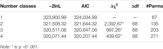
TABLE 6. Log likelihoods and fit indices for the partial credit and mixture partial credit models from node scores.

TABLE 7

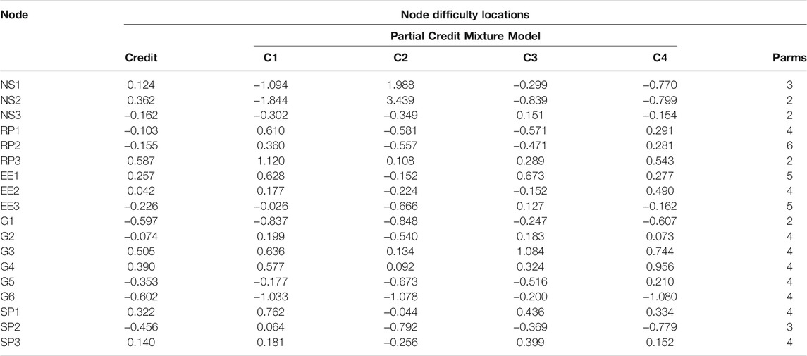
TABLE 7. Item difficulty locations for the partial credit models for node scores.

Mixture partial credit model.Table 6 also shows the log likelihoods, AIC values, and significance tests for increasing numbers of classes. For example, estimating two classes with varying patterns of node location difficulties resulted in a highly significant difference in fit as compared to the single-class solution (Δχ² = 2,392.67, df = 68, p <0 .001). Significant differences were found increasing the number of classes up to four. However, beyond this point, increasing the number of classes yielded classes involving fewer than 10 percent of the students. With the four-class solution, person fit, as indicated by a person’s highest class probability (i.e., ${\eta }_{mj}$ in Eq. 5 above), had a mean of 0.811, supporting strong fit.

Table 7 presents the node location difficulty levels for the partial credit model and the partial credit mixture model in the four-class solution, which are also plotted on Figure 6. As for binary data, the mean item difficulty is zero in the partial credit model and within classes of the mixture model. However, substantial differences in the relative difficulty of the nodes within the four classes was observed. Figure 6 shows that the node difficulty locations vary the most between the classes in the number sense and ratio area. Class 2, for example, had much higher estimated difficulties for two number sense and ratio nodes. The most extreme difference is for NS2, which ranges from −1.844 to 3.439 across classes. However, differences between the classes in many other areas, although much smaller, also could be sufficient to produce estimated differences in student mastery.

FIGURE 6

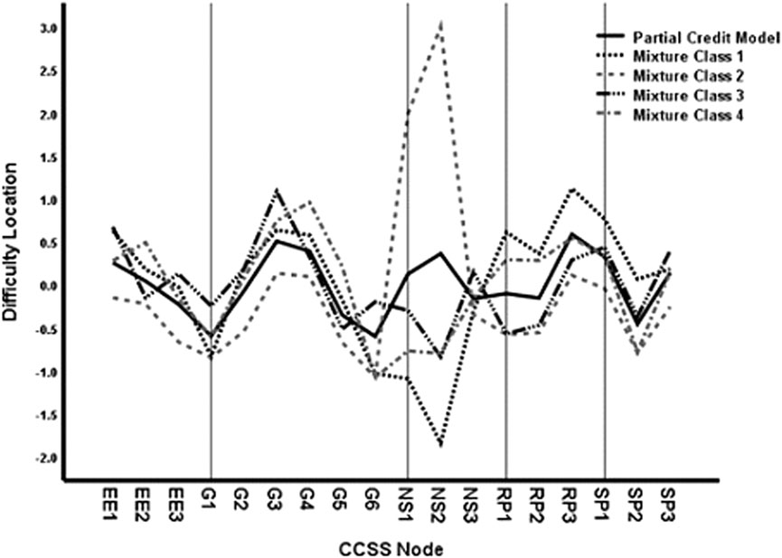
FIGURE 6. Node difficulty locations by class for node score data.

Table 8 presents results on trait levels in the four-class solution for node scores. It can be seen that Class 1 has the highest proportion of students and substantially higher mean trait levels as compared to the other classes. The lowest trait level mean is for students in Class 3. The empirical reliabilities of trait level scores in the various classes are high, although Class 1 had a somewhat lower reliability. Table 8 shows that the mean probability for solving items in Class 1 was very high. Thus, few items in the nodes were sufficiently difficult for their trait levels which led to relatively larger standard errors and lower overall reliability.

TABLE 8

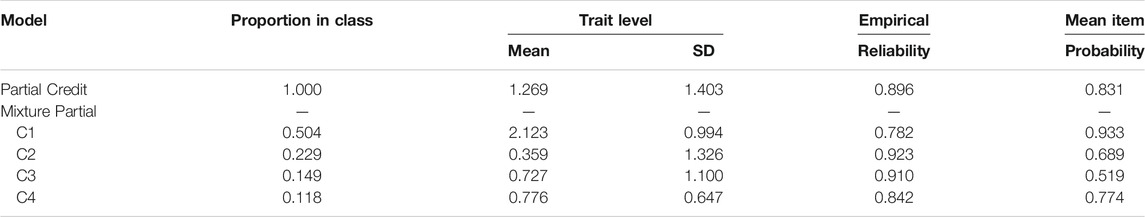
TABLE 8. Trait level means, standard deviations, empirical reliabilities, and item-solving probabilities in the partial credit and partial credit mixture models.

Differential diagnosis. Parameter estimates from the two models, the partial credit model and the four-class mixture partial credit model, were used to predict the expected node scores for each student based on trait level and node difficulty thresholds. These scores were divided by the number of items in the node to yield a probability for item solving in each node. As for item accuracy scoring above, if the probability equaled or exceeded 0.70, the student was deemed to have mastery.

The mastery versus non-mastery expectations for each node were then compared between the two models. Figure 7 shows the proportion of students for which the two models yielded different mastery expectations for each node. It can be seen that several nodes in number sense and ratios differed substantially. For NS2, for example, more than 30% of the students had a different diagnosis of mastery from the two models. Nodes in other areas, such as SP1 and G6, also differed in predictions from the two models.

FIGURE 7

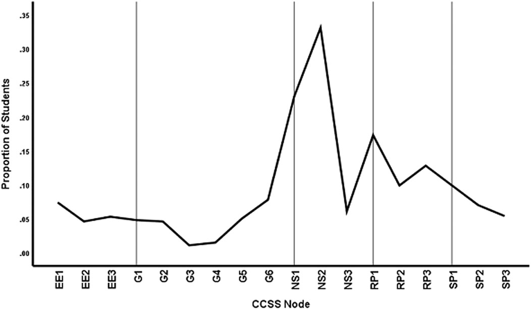
FIGURE 7. Proportion of students with differential diagnosis by method and CCSS node at cutline70 for node score data.

Discussion

The purpose of the current study was to examine the use of varying IRT models to predict students’ mastery of specific learning map nodes from a comprehensive achievement test. Such tests are routinely administered in elementary and middle schools to assess overall achievement at the end of the school year. The wide availability of the tests could make them practical for determining needed remedial instruction. However, the available overall scores are useful for diagnosing mastery of specific learning map nodes only if the various total score levels have the same implications for area and node mastery. Typically, this is not the case. Sub-scores are often computed to examine performance in various achievement areas. These scores are typically less reliable but also not sufficiently precise, particularly if the pattern of mastery of nodes within areas varies across students.

The results of the current study confirm these problems, as both model fit and score reliability varied across models. That is, using binary-scored items, a multidimensional IRT model based on the content areas fit significantly better than a unidimensional model. Thus, varying patterns of content area mastery for the students was supported. However, as expected, score reliability was substantially reduced. The unidimensional model trait scores had reliability of 0.903 while the multidimensional trait score reliabilities ranged from 0.462 to 0.765. Worse, however, the less reliable area sub-scores can be used to predict item probabilities for ELM learning map nodes only if students have the same pattern of node mastery within areas. This was not supported in the analysis with mixture IRT models.

That is, the analysis with mixture class IRT models suggested that at least four distinct latent classes of examinees were needed to fit the varying patterns of item accuracy data. The latent classes varied not only in the relative difficulty of the four areas of the test items, consistent with the multidimensional IRT model, but also differed in the relative difficulty of specific nodes within areas. Importantly, the observed differences in mastery patterns between the classes were not strongly impacted by unreliable estimates of trait level. That is, the reliabilities of trait scores for the four-class mixture model were acceptable, ranging from 0.750 to 0.897. Thus, the mixture class model for item accuracy not only fit substantially better, but also the node-specific predictions of mastery were based on more reliable trait scores.

Further analysis showed differential diagnosis of node mastery between the three IRT models for item accuracy. Approximately the same overall proportion of students were found to have mastery of the various nodes across models; however, the models differed in which students were predicted to have mastery.

Similar results were found for mixture IRT models using the polytomous items that represented node scores. Statistically significant improvements in fit were found by increasing the number of latent classes for the partial credit IRT model. As for the binary-scored item data, four latent classes were supported to improve model fit. Thus, varying patterns of node difficulty for different students was supported. Also, as for the binary item data, the reliability of trait level scores was acceptable across classes, ranging from 0.782 to 0.923. However, for the polytomous items, node difficulty differences were more directly relevant to defining the latent classes. The difficulty of nodes within number sense and ratio areas differed most strongly between classes. Further, differential diagnosis of these nodes in the mixture model, as compared to the unidimensional partial credit model, was especially strong.

Overall, the results indicate that using mixture class IRT models, in conjunction with parameter-based predictions, improves the prediction of mastery at the node level from comprehensive achievement tests. Particularly interesting are the results using polytomous node-scored items to provide the parameter estimates in the latent classes. That is, reliable trait scores were obtained and the latent classes were based directly on the varying patterns of node difficulty for different students. The results are also likely to apply to more area-specific interim tests for diagnosing mastery because node differences within areas were found.

However, the results from the polytomous mixture model did vary somewhat from the binary mixture models. That is, the classes and subsequent differential diagnosis obtained from the polytomous data (i.e., Figure 7) differs somewhat from the classes and diagnosis from the binary data (i.e., Figure 5). If the goal is to determine node differences, the polytomous data is preferable, but it must be assumed that the items within the nodes all represent the specified standards. In contrast, the classes resulting from the binary data will reflect both node pattern differences and unintentional within node item differences. Future research should examine further the impact of item correspondence to node definitions on these models.

One area for future research is to explore the basis of varying patterns of mastery, especially as defined by the mixture IRT models. Variables that may impact instruction, such as urban versus rural districts or teacher training, should be examined for relationship to the latent class membership of their students. Student background variables, such as gender, race-ethnicity, and native language, may also impact varying patterns of node difficulty and should be examined in future studies.

Importantly, future research also should examine the usefulness of mastery diagnosis of specific learning map nodes from comprehensive achievement tests using the modeling approaches in this study. Two outcome variables that are especially important to relate to mastery diagnosis are 1) the predictability of mastery based on longer tests that are associated with specific nodes and 2) the relative outcomes of remedial instruction for different mathematical standards. The results of the current study would suggest that the mixture models would be more useful than either the unidimensional and area-specific multidimensional approaches.

Data Availability Statement

The data analyzed in this study is subject to the following licenses/restrictions: Available to the author only. Requests to access these datasets should be directed to Not available

Ethics Statement

Ethical review and approval was not required for the study on human participants in accordance with the local legislation and institutional requirements. Written informed consent from the participants’ legal guardian/next of kin was not required to participate in this study in accordance with the national legislation and the institutional requirements.

Author Contributions

The author confirms being the sole contributor of this work and has approved it for publication.

Conflict of Interest

The author declares that the research was conducted in the absence of any commercial or financial relationships that could be construed as a potential conflict of interest.

Publisher’s Note

All claims expressed in this article are solely those of the authors and do not necessarily represent those of their affiliated organizations, or those of the publisher, the editors, and the reviewers. Any product that may be evaluated in this article, or claim that may be made by its manufacturer, is not guaranteed or endorsed by the publisher.

References

GMADE and Pearson (2018). Group Mathematics Assessment and Diagnostic Evaluation. Available at: https://www.pearsonassessments.com/.

Google Scholar

Hess, K., Kurizaki, V., and Holt, L. (2009). Reflections on Tools and Strategies Used in the Hawai’I Progress Maps Project: Lessons Learning from Learning Progression. Report for Tri-state Enhanced Assessment grant. Available at: https://nceo.umn.edu/docs/tristateeag/022_HI%201.pdf

Google Scholar

Kansas State Department of Education (2017). The 2017 Kansas Mathematics Standards:Grade K-12. Available at: https://community.ksde.org

Google Scholar

Kingston, N., and Broaddus, A. (2017). The Use of Learning Map Systems to Support the Formative Assessment in Mathematics. Edu. Sci. 7 (41), 41. doi:10.3390/educsci7010041

CrossRef Full Text | Google Scholar

Kingston, N. M., Karvonen, M., Bechard, S., and Erickson, K. (2016). The Philosophical Underpinnings and Key Features of the Dynamic Learning Maps Alternate Assessment. Teachers College Record (Yearbook), 118, 140311. online Available at: http://www.tcrecord.org

Google Scholar

Li, H. (2011). A Cognitive Diagnostic Analysis of the MELAB reading Test. Spaan Fellow Working Pap. Second or Foreign Lang. Assess. 9, 17–46.

Google Scholar

Nations Report Card (2019). NAEP Item Maps: Mathematics, Grade 4. online Available at: http://www.nationsreportcard.gov/nationsreportcard/itemmaps/

Google Scholar

Pan, Q., Qin, L., and Kingston, N. (2020). Growth Modeling in a Diagnostic Classification Model (DCM) Framework-A Multivariate Longitudinal Diagnostic Classification Model. Front. Psychol. 11, 1714–1717. doi:10.3389/fpsyg.2020.01714

PubMed Abstract | CrossRef Full Text | Google Scholar

Popham, W. J., Berliner, D. C., Kingston, N., Fuhrman, S. H., Ladd, S. M., Charbonneau, J., et al. (2014). Can Today's Standardized Tests Yield Instructionally Useful Data? Challenges, Promises and the State of the Art. Qual. Assur. Edu. 22 (4), 300–316. doi:10.1108/qae-07-2014-0033

CrossRef Full Text | Google Scholar

R. Cameto, S. Bechard, and P. Almond (Editors) (2012). “Understanding Learning Progressions and Learning Maps to Inform the Development of Assessment for Students in Special Populations,” in Third Invitational Research Symposium, Menlo Park, CA, and Lawrence, KS. (SRI International and Center for Educational Testing and Evaluation (CETE)).

Google Scholar

Rost, J., and von Davier, M. (1995). “Mixture Distribution Rasch Models,” in Rasch Models. Editors G.H. Fischer, and I.W. Molenaar (New York, NY: Springer), 257–268. doi:10.1007/978-1-4612-4230-7_14

CrossRef Full Text | Google Scholar

Rupp, A. A., Templin, J. L., and Henson, R. A. (2010). Diagnostic Measurement: Theory, Methods, and Applications. New York: The Guilford Press.

Thissen, D., Steinberg, L., and Mooney, J. A. (1989). Trace Lines for Testlets: A Use of Multiple-Categorical-Response Models. J. Educ. Meas. 26, 247–260. doi:10.1111/j.1745-3984.1989.tb00331.x

CrossRef Full Text | Google Scholar

Wilson, M., and Bertenthal, M. (2005). Systems For State Science Assessment. Board on Testing and Assessment, Center for Education, National Research Council of the National Academics. Washington, DC: National Academics Press.