Multilevel Latent Transition Mixture Modeling: Variance Decomposition and Application

Person-centered methodologies generally refer to those that take unobserved heterogeneity of populations into account. The use of person-centered methodologies has proliferated, which is likely due to a number of factors, such as methodological advances coupled with increased personal computing power and ease of software use. Using latent class analysis and its extension for longitudinal data, [latent transition analysis (LTA)], multiple underlying, homogeneous subgroups can be inferred from a set of categorical and/or continuous observed variables within a large heterogeneous data set. Such analyses allow researchers to statistically treat members of different subgroups separately, which may provide researchers with more power to detect effects of interest and closer alignment between statistical modeling and one’s guiding theory. For many educational and psychological settings, the hierarchical structure of organizational data must also be taken into account; for example, students (i.e., level-1 units) are nested within teacher/schools (i.e., level-2 units). Finally, multilevel LTA can be used to estimate the number of latent classes in each structured unit and the potential movement, or transitions, participants make between latent classes across time. The transitions/stability between latent classes across time can be treated as the outcome in and of itself, or the transitions/stability can be used as a correlate or predictor of some other, distal outcome. The purpose of the paper is to discuss multilevel LTA, provide considerations for its use, and demonstrate variance decomposition, which requires numerous steps. The variance decomposition steps are presented didactically along with a worked example based on analysis from the Social Rating Scale of ECLS-K.

1 Introduction

Efforts to classify individual cases into homogeneous groups have long been used in order to better understand complex sets of information. Classification of cases into homogeneous groups has important implications in the social sciences, such as education, medicine, psychology, or economics, where identifying smaller subsets of like cases may be of particular interest. Person-centered methodologies generally refer to those that take unobserved heterogeneity of populations into account. That is, rather than treat all individuals as if they originated from a single underlying population, as is true with variable-centered methodologies, person-centered methodologies allow for multiple subpopulations to underlie a set of data. The challenge with these methods is identifying the correct number (i.e., frequency) of subpopulations, or classes, and the parameters (i.e., form) associated with each, when the frequency and form are not known a priori (Nylund et al., 2007; Tofighi and Enders, 2008; Morgan, 2015).

Mixture modeling, generally, refers to the family of statistical procedures for identifying homogeneous subpopulations of cases from one large, heterogeneous data set (McLachlan and Peel, 2004; Collins and Lanza, 2009). The analysis assumes that an observed dataset is a mixture of observations collected from a finite number of mutually exclusive classes, each with its own characteristics. These procedures have been referred to in the literature under many different names, such as mixture likelihood approach to clustering (McLachlan and Basford, 1988; Everitt, 1993) and model-based clustering (Banfield and Raftery, 1993). Depending on the metric level of the variables included in the study, other terms used to describe this methodology are latent class analysis, latent profiles analysis, latent class clustering, or model-based clustering.

Many advances have occurred in mixture modeling as an analytic methodology, which now includes models like factor mixture, growth mixture, diagnostic classification, and latent Markov models. Moreover, mixture modeling is now being applied in fields ranging from education to brain imaging and geosciences to robotics. Despite the proliferation of models and applications that fall within the mixture modeling framework, there are still new areas and angles to explore and better understand in order to more fully realize the strengths of this analytic framework. One such area where limited research has been disseminated involves nested data structures that are collected longitudinally. That is, multilevel mixture models are available to researchers although they have not been discussed as extensively as other cross-sectional and longitudinal mixture models. Asparouhov and Muthén (2008) and Kaplan et al. (2011) presented findings from applications of this type of model, but additional guidance on the use of these models may help users better understand their data structures and, ultimately, make better decisions about their research questions. One important consideration when using these models is the ability of the researcher to understand the magnitude and sources of effects through the decomposition of variance. This is especially true in models, such as the ones we present in the next section, that have nested data structure collected across time.

This is precisely the purpose of this paper. That is, we seek to 1) present and discuss multilevel latent transition analysis, 2) describe considerations for the use of this model, and 3) demonstrate a multi-step variance decomposition. The variance decomposition steps are presented didactically along with a worked example based on an analysis from the Social Rating Scale (SRS) of Early Childhood Longitudinal Survey - Kindergarten (ECLS-K). Several additional notes are important due to the didactic nature of this paper. First, the latent class analysis and latent profile analysis differ on the basis of the metric level of the indicator variables, yet these are conceptually similar analyses. Latent categorical variables are often referred to as latent classes regardless of the metric level of the indicator variables. As such, there are instances where we use “class” and “profile” interchangeably. For this paper, we are modeling continuous indicators so the term “latent profile” is most precise, but the discussion and procedures we present apply to model with categorical and/or continuous indicators. Second, we demonstrate the procedures for variance decomposition with a two-class model for didactic reasons; therefore, any substantive conclusions about the specific variables or participants used in the example should be avoided. Third, we used the Grades 3 and 5 SRS scores from restricted-use ECLS-K 1998 datafile; the scores for Grades 3 and 5 were respectively collected in Spring 2002 and Spring 2004.

2 Introduction to Latent Transition Analysis

When using latent class analysis and its extension for longitudinal data, [latent transition analysis (LTA)], multiple underlying, homogeneous subgroups can be inferred from a set of categorical and/or continuous observed variables within a large heterogeneous data set. Such analyses allow researchers to statistically treat members of different subgroups separately, which may provide researchers with more power to detect effects of interest and closer alignment between statistical modeling and one’s guiding theory.

In latent class analysis (LCA), membership in one of the underlying populations is conceptualized as a latent, categorical variable that is not directly observed. Instead, latent class membership must be measured using two or more observed, or indicator, variables, taken as a manifestation of latent variables. The number of latent profiles underlying a dataset is not known a priori, and thus, has to be uncovered (Collins and Lanza, 2009). The process typically involves fitting models that specify different numbers of profiles in order to determine which model best approximates the heterogeneous set of data. Each case is assigned a probability of belonging to each profile based on the alignment between the characteristics (e.g., response probabilities, means, variances, covariances) between each case and each profile. When the characteristics of a case are similar to those of a given profile, the case has a high probability of being a member of the subpopulation. When the characteristics of a case are dissimilar to those for a stated profile, the case has a low probability of belonging to the profile. Generally, cases are assigned to the profile to which they have the highest probability of belonging, which is called modal assignment (Collins and Lanza, 2009). Ideally, the classification probability for each person will be high for one and only one profile. An optimal solution will have high classification probabilities for each latent class, illustrating that the classes are distinct.

The procedures described above can be applied to cross-sectional data or data collected at multiple points in time. LTA, the longitudinal extension of LCA, allows the stability of an LCA solution to be examined across time. Furthermore, LTA allows researchers to examine transition patterns among latent classes across time using one of several strategies. The first strategy is to regress latent class membership at time $t+1$ on latent class membership at time t, which is analogous to a multinomial regression. When three or more Waves of data collection are completed, this strategy can be done with or without higher-order effects, which enables a researcher to explore the lasting direct effects of latent profile membership on later profile membership through an autoregressive model (Nylund et al., 2007). However, in this paper we restricted our investigation to two timepoints for didactic purposes and only a one lag autoregression structure is possible. A second strategy is to include a second-order latent class variable that identifies participants who are most likely to switch latent classes (i.e., movers) or remain in the same class (i.e., stayers) across time. Such models have been referred to as a mover-stayer LTA model. The mover-stayer model is an extension of the Markov chain model and special case of the mixed Markov model. Interested readers should see Blumen et al. (1955) and Goodman (1961) for a thorough presentation of the mover-stayer model and Vermunt (2004) for a great summary of the model. The mover-stayer model and its variants could be considered when certain types of transition are of interested, such as first marriage or death, where transition back to a previous state is not possible or when transition is believed to occur by a random process Vermunt (2004). The mover-stayer model can be more parsimonious but its selection should ultimately be aligned with one’s guiding theoretical expectation and associated research questions.

The modeling strategy chosen has important implications on the structure of the latent transition matrix, which contains probabilities of transitioning to another latent class conditioned on latent class membership at 1) time 1 if only two waves of data collection occurred or 2) $t-1$ if used with more than two waves of data collection. In the former option, the transition matrix is unstructured, which allows any transition pattern to take place. In the latter option, the diagonal of the transition matrix is constrained to 1.0 among the stayers, which assigns those participants classified as stayers a transition probability of zero of switching to another profile (Morgan, 2015).

2.1 Multilevel Latent Transition Analysis for Longitudinal Nested Data

Although LTA accounts for the collection of data from the same individuals across time (i.e., time nested within person), the model can also be extended to account for individuals being nested within higher level units, such as schools, hospitals, organizations, etc. In education research, statistical methods are commonly used that model students nested within schools, which is the context for the illustration in this paper. In such cases, the hierarchical structure of organizational data must be taken into account because independence between observations is not tenable; that is, students (i.e., level-1 units) are nested within and share influence of schools (i.e., level-2 units). Thus, multilevel LTA can be used to estimate the number of latent classes in each structured unit and the transitions participants make between classes across time. Finally, the transitions/stability between latent classes across time can be treated as the outcome in and of itself, or the transitions/stability can be used as a correlate or predictor of some other, distal outcome.

The multilevel LTA can be expressed as a series of multinomial logistic regressions at level-1 and as a linear regression at level-2 (Asparouhov and Muthén, 2008). To illustrate, consider the model below that has two latent classes across two time points. At level-1 the multinomial logistic regression for the latent classification variable at time 1, $C_1=\mathrm{1,2}$, can be expressed as

$\mathrm{P}\left(C_{1ig}=1\right)=\frac{\exp \left({\alpha }_{1g}\right)}{\exp \left({\alpha }_{1g}\right)+1},(1)$

where $C_{1ig}$ represents the latent class at time 1 for individual i in group g, and ${\alpha }_{1g}$ is the intercept of latent class 1 for group g and is assumed to be normally distributed. The intercept for latent class 2 at time 1 is set to zero for identification because only one intercept is needed to distinguish two latent classes. The multinomial logistic regression of latent class at time 2 ($C_2$) on latent class at time 1 ($C_1$) can be expressed as

$\mathrm{P}\left(C_{2ig}=1|C_{1ig}=c\right)=\frac{\exp \left[{\alpha }_{2g}+\gamma I\left(C_{1ig}=1\right)\right]}{\exp \left[{\alpha }_{2g}+\gamma I\left(C_{1ig}=1\right)\right]+1},(2)$

where ${\alpha }_{2g}$ represents the latent class intercept at time 2 for individual i in group g, and γ represents the expected change in logits from the multinomial logistic regression predicting latent class at time 2 from latent class at time 1. The indicator function ($I\left(C_{1ig}=1\right)$) in Eq. 2 demonstrates how the latent regression parameter γ is specific to class 1 which is how class specific transition probabilities are captured in the model (Asparouhov and Muthén, 2008; Kaplan et al., 2011). That is, the indicator function takes on values $\left\{\mathrm{0,1}\right\}$ depending on whether or not latent class membership at time 1 was equal to 1. Like the latent class intercept for class 2 at time 1, the latent class intercept for class 2 at time 2 is set to zero for identification. It should be noted the number of regression weights, γ, increases as the number of latent classes increases. For example, two latent classes implies one γ whereas three classes implies up to four γs. Additionally, the model above can be extended to incorporate student level covariates into the transitional structure (Vermunt et al., 1999).

The multinomial autoregression model above is akin to what is used in single-level LTA; however, a unique contribution of multilevel LTA is the incorporation of a latent regression model of latent class intercepts over time. At level-2, the random effects of latent class size across schools can be explained as part of a series of latent linear regression models such as

${\alpha }_{1g}={\mu }_{{\alpha }_1}+{\epsilon }_{{\alpha }_1}(3)$

${\alpha }_{2g}={\mu }_{{\alpha }_2}+\beta {\alpha }_{1g}+{\epsilon }_{{\alpha }_2}.(4)$

The regression in Eq. 3 models the difference in latent class size across schools at time 1 where ${\alpha }_{1g}$ is the latent class size in logits for school g at time 1, ${\mu }_{{\alpha }_1}$ is the average latent class size at time 1, and ${\epsilon }_{{\alpha }_1}$ is random effect of latent class size across schools. Similarly, the regression in Eq. 4 models the differences in latent class size across schools at time 2, where ${\alpha }_{2g}$ is the latent class size in logits for school g at time 2, ${\mu }_{{\alpha }_2}$ is the average latent class size at time 2 unconditional on latent class size at time 1, β is the fixed effect of latent class size at time 1 on time 2 latent class size, and ${\epsilon }_{{\alpha }_2}$ is the random effect of latent class size across schools unique to time 2. The random effects are commonly assumed to be normally distributed with unique variance estimates at each timepoint [e.g., $\text{var}\left({\alpha }_1\right)$ and $\text{var}\left({\alpha }_2\right)$]. The level-2 latent regression of the multilevel LTA model expresses how latent class sizes change over time among schools. Factors that influence differences in latent class size over time among schools can be studied in more detail if level-2 covariates are included in the model. The incorporation of covariates can be guided by substantive interest and by information about how much information can be accounted for by these covariates. The amount of information that is contained in the level-2 portion of the model can be expressed by different $R^2$-like measure that can be computed.

The multilevel LTA model has many parameters to describe the process which generated the differences in observed characteristics across time, and some of the model features are directly interpretable whereas other features are less easily interpreted. In order to help explain the complex features of the model, various $R^2$-like measures can be computed to provide information about how the variability in latent class membership is influenced by 1) time, 2) nested data structure, and/or 3) individual latent class membership. For example, Asparouhov and Muthén (2008) and Kaplan et al. (2011) explicitly described an $R^2$ measure for the proportion of variance in latent class membership at time 2 that is accounted for by latent class membership at time 1. And is readily available for use in single-level LTA as well. This $R^2$ measure is

$R^2=\frac{{\gamma }^{2}P\left(C_1=1\right)\left(1-P\left(C_1=1\right)\right)}{{\gamma }^{2}P\left(C_1=1\right)\left(1-P\left(C_1=1\right)\right)+{\pi }^2/3},(5)$

where $P\left(C_1=1\right)$ is the probability of being latent class 1 at time 1 and ${\pi }^2/3$ is the residual variance associated with the logistic regression performed at level-1. $P\left(C_1=1\right)$ may also be viewed as the relative size of latent class 1 at time 1. Although the result in Eq. 5 is useful, there is more information in a multilevel LTA model that can be used to gain additional insights into the process under investigation.

Asparouhov and Muthén (2008) used these other $R^2$-like measures, such as the proportion of variance in $C_1$ explained by ${\alpha }_1$, the proportion of variance in $C_2$ explained by the group effect at time 1, among others, but they did not describe the steps necessary to calculate these values. A detailed explanation on how to obtain such $R^2$-like measures is therefore one of the major contributions of this work.

One potential limitation of the $R^2$ measure in Eq. 5 is that the hierarchical structure of the data is ignored, which means that it may overestimate the effect latent class membership at time 1 has on latent class membership at time 2. The methods we demonstrate for decomposing the variance in multilevel LTA explicitly account for this feature of the data. That is, the variance decomposition we describe accounts for the nested data structure by incorporating all model components into the variability in latent class membership at time 2.

2.2 Considerations for Using Multilevel Latent Transition Analysis

There are several considerations specific to multilevel LTA that extend beyond those associated with LCA and LTA. First, one must consider whether the research question posed requires the multilevel aspect of the data explicitly incorporated into a mutlilevel LTA model. Not all questions require that the nested nature of the data be explicitly modeled (McNeish et al., 2017). For example, a researcher primarily interested in transitions of students among latent classes over time may not need to explicitly account for a school effect if differences among schools does not influence the students’ transitions. Instead, the multilevel aspect of the data can be incorporated implicitly through the use of sampling weights (Stapleton, 2013) or alternatives such as cluster-robust standard errors (McNeish et al., 2017). However, the use of multilevel LTA is likely warranted when researchers believe that characteristics of the group or school are related to differences in latent class membership. This is commonly encountered in education and healthcare applications where between-school and between-hospital differences, respectively, influence large groups of participants simultaneously.

In additional to the nested feature of one´s data, another important consideration is the time scale in which data were collected. The time scale of data collection may, or may not, adhere time scale of the transitions that individual may experience. Collins and Lanza (2009, p. 209–211) expressed how the transition structure estimated may reveal only chance transitions due to a underlying structure that transitions very rapidly (e.g., the example of indicators of depression in the last week but data were collected one year apart). Therefore, researchers must think carefully about how observed transitions among latent classes are related to transitions in the underlying construct of interest. In multilevel LTA, in particular, an additional consideration is whether the time scale of the transition is equal across level-2 units, such as schools. In healthcare settings, for example, the time scale of transitioning among depression latent classes may depend in part on the care received across different clinics if clinics were to have a general approach to helping patients with, say, depressive symptoms. As noted above, these considerations should be applied in addition to those important considerations that have been identified for LCA and LTA, such as model selection (Nylund et al., 2007; Tofighi and Enders, 2008; Morgan, 2015), label switching (Chung et al., 2004; Tueller et al., 2011), nature of the latent variables (Lubke and Neale, 2008), and incorporation of distal outcome (Lanza et al., 2013; Bakk and Vermunt, 2016; Nylund-Gibson et al., 2019). An excellent collection of applied and methodological papers using these procedures can be found on the Mplus website (www.statmodel.com/paper.shtml).

Next, we illustrate the use of multilevel LTA and explicitly model the multilevel nature of the data.

3 Application of Multilevel Latent Transition Analysis

3.1 Sample

The data used are a subset of the ECSL-K national dataset (Tourangeau et al., 2009). The analytic sample for this demonstration was approximately 7,080 students nested within approximately 1,100 schools (sample sizes have been rounded to the nearest 10 in compliance with federal restricted-use data reporting guidelines). Prior to estimating the multilevel LTA model, we subset the ECLS-K data file on the students who remained in the same school from at least Grade 3 to Grade 5. The average number of students per school was 6.4 ($SD=5.3$) and ranged from 1 to about 30 students.

3.2 Instrumentation

In order to demonstrate the model output and subsequent decomposition of the model variance, we used the five Social Rating Scale subscales from the Early Childhood Longitudinal Survey–Kindergarten (ECLS-K) data. The five major constructs of interests are: Approaches to Learning (AtL), Self-Control (SC), Interpersonal Skills (IPS), Externalizing Problem Behaviors (EPB), and Internalizing Problem Behaviors (IPB) (Tourangeau et al., 2009). These five constructs of child behaviors/characteristics are modeled as being reflective of a child’s need for possible additional behavioral intervention. The reliability estimates (coefficient α) for these constructs in the full ECLS-K in spring of fifth grade ranged from 0.77 (Internalizing Problem Behaviors) to 0.91 (Approaches to Learning). Reading teachers were asked to report how frequently students exhibited the social skill or behavior identified by each item. The response scale used a four-point frequency scale ranging from 1 (Never) to 4 (Very Often). The same 26 SRS items administered in Grade 3 and 5. A summary of these raw subscale scores is shown in Table 1.

TABLE 1

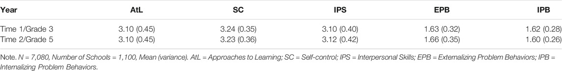
TABLE 1. Summary of observed data.

The raw subscale scores were computed as the average of the responses to the items on each subscale.

3.3 Procedures

The model was estimated using maximum likelihood estimator with robust standard errors (MLR) in Mplus v8.4 (L. Muthén and Muthén, 2017) using 2,000 random starting values and 50 final stage optimizations. For illustrative purposes, we estimated only a two-class solution. In practice, additional class enumeration models would be estimated and compared. For this demonstration, we elected to not use sampling weights to reduce the complexity of the example analysis. All inferences from the following model are restricted to this sample of students and is not necessarily a representation of the characteristics of students more broadly.

The path diagram for the multilevel LTA model is presented in Figure 1. We should note that the path diagram includes variance components to aid in interpretation of variance decomposition discussion below.

FIGURE 1

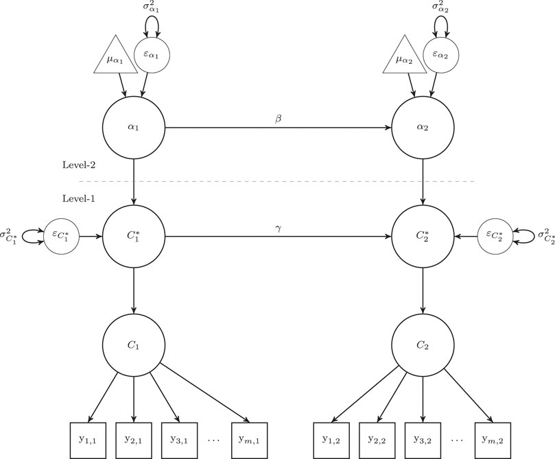
FIGURE 1. Path diagram of a multilevel latent transition model proposed for ECLS-K Social Rating Scale over two waves. Note. Subscripts indicate the timepoint of the data. AtL = Approaches to Learning; SC = Self-control; IPS = Interpersonal Skills; EPB = Externalizing Problem Behaviors; IPB = Internalizing Problem Behaviors; ${\alpha }_t$ = random intercept for time t, so ${\alpha }_1$ is the random intercept time 1; $C_t$ = latent class at time t, which takes on values $C_t=\mathrm{1,2}$ (For ease of notation, let $c=\mathrm{1,2}$ represent latent class at time 1 and let $d=\mathrm{1,2}$ be the latent class at time 2); β = the regression weight associated of random effect at time 1 predicting the random effect at time 2; γ = the change in logits of the latent response tendency variable at time 2 for individuals in class 1 at time 1 (γ only applied to cases that are in class 1 at time 1 which is captured by using an indicator function $I\left(C_1=1\right)$ which is a Bernoulli random variable); the residual variance of the level-1 latent response tendency variable relative to the reference class, $C_t^{\text{*}}$ is $\frac{{\pi }^2}{3}=3.29$ which is the variance of the logistic distribution.

The major inferential goals are the evaluation of the transition parameters ($\gamma ,\beta$) and the variability in latent class size across schools ($\text{var}\left({\alpha }_1\right),\text{var}\left({\alpha }_2\right)$).

3.4 Results

The resulting latent class patterns are shown in Table 2. In the estimation, the latent class structure was fixed to be invariant across time. Latent class 1 is characterized by students who had lower ratings on the three positive constructs (i.e., AtL, SC, and IPS) and higher scores on the constructs reflecting problem behaviors (i.e., EPB and IPB). Latent class 2 was characterized as having higher scores on the three positive constructs (i.e., AtL, SC, and IPS) and lower ratings on the problem behavior constructs (i.e., EPB and IPB).

TABLE 2

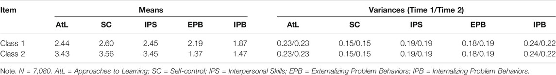
TABLE 2. ECLS-K 2-class model of social rating scale measurement model.

The structural model parameters are described in Table 3. At Time 1, Class 1 was the smaller of the two latent classes, making up about 32% of the sample, whereas Class 2 made up about 68% of the sample. Due to the multilevel nature of the data, the parameter estimate, $\text{var}\left({\alpha }_1\right)=0.64$, offers additional insights into the latent class structure at time 1. That is, the estimate of 0.64 suggests the proportion of students in Class 1 and Class 2 at time 1 varies depending on the school. In other words, Class 1 contains about 32% of the students at time 1, on average, but this percentage differs across schools with a 95% probable range of 9–69%. The larger the variance estimate, the greater the school effect and greater range of relative class sizes across schools.

TABLE 3

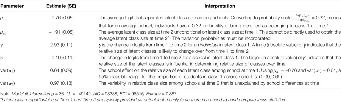
TABLE 3. ECLS-K 2-class multilevel LTA model of social rating scale results and interpretation.

The transition component of the multilevel LTA model is characterized by the parameters γ ($\gamma =2.93,SE=0.11,p<0.001$) and β ($\beta =-0.19,SE=0.11,p=0.077$). From these two parameters, a transition matrix ($\mathit{\tau }$) is constructed to help explain the overall effect of time. The details of computing these values are given in the Multilevel LTA Variance Decomposition section; but for now, these results are reported in Table 4 along with the interpretation. We found that the, on average, about 13% of students who were classified in Class 2 at Time 1 (i.e., third grade) transitioned into the Class 1 at Time 2 (i.e., fifth grade). Of those students classified in the Class 1 at Time 1, approximately 26% transitioned into Class 2.

TABLE 4

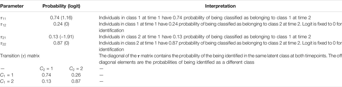
TABLE 4. Transition structure interpretation for an 2-class multilevel LTA model.

As alluded to above, there are numerous calculations necessary to extract important modeling results that guide interpretation. The intraclass correlation (ICC) estimate for this model indicates that about 16% proportion of variability in class assignment at Time 1 can be explained by the school effect. Using the variance decomposition, 10.4% of the variability in latent class membership at Time 2 can be accounted for by the school effect at Time 1. However,15.8% of the variability in latent class membership at Time 2 can be accounted for by the school effect at Time 2. The incorporation of school level covariates into Eq. 3 and Eq. 4 could give insight into what school characteristics are associated with latent class membership at Time 2 by investigating the change in the previous two $R^2$ measures in models estimated with and without the covariate included. At the student level, the class assignment at Time 1 accounted for about 30.3% of the variability in class assignment at Time 2. The unexplained variability in class assignment at Time 1 also accounted for about 53% of the variability in class assignment at Time 2. Overall, the multilevel LTA model without any covariates explained approximately 46.5% of the variance in class assignment at Time 2. Finally, the inclusion of the multilevel structure explained about 16.2% of the variability in latent class membership at Time 2.

4 Multilevel Latent Transition Analysis Variance Decomposition

Clearly, as indicated above, examining the proportion of variability that can be attributed to each component of the model can aid in interpreting the model effects. Although the parameter estimates provides some indication of the magnitude of model effects, the scale can make them difficult interpret. Furthermore, it is customary in traditional regression to report the proportion of variability explained by the model, and in multilevel models reporting the proportion of variability that is attributable to higher- and/or lower-level units can greatly inform inferences about the magnitude of effects of those units on the outcome(s) of interest. In this didactic model, for example, the estimated regression weight for the effect that latent class membership in Grade 3 had on latent class membership in Grade 5, controlling for school-level effects, was 2.93. Is this effect small, moderate, or large? It is difficult to make such a determination with the effect on this metric. Decomposing the variance and reporting the effect as a percentage makes the effect much easier to interpret. That is, the proportion of variability of $C_2$ explained by $C_1$ is about 30.3%. Considering that the model explained about 46.5% of the total variability in $C_2$, school-level variables accounted from 16.2% of the variance in $C_2$. Thus, the school-level variables accounted for more than one-third of all the variability explained by the model.

Due to the didactic nature of this paper, we refrain from commenting on any substantive conclusions regarding the size of this effect; rather, we seek to demonstrate how the variance decomposition produces a more intuitive, or at least familiar, effect size estimate. That said, certain $R^2$-like measures could be calculated for various effects in the model, including at each timepoint (i.e., transition) and for the overall model. Next, we demonstrate the steps required in the decomposing the model variance using the parameter estimates the multilevel LTA model (${\mu }_{{\alpha }_1}=-0.76$, ${\mu }_{{\alpha }_2}=-1.91$, $\text{var}\left({\alpha }_1\right)=0.64$, $\text{var}\left({\alpha }_2\right)=0.97$, $\gamma =2.93$, and $\beta =-0.19$) to calculate the effect sizes reported in the Results section as estimates of the proportions of variance explained in latent class membership at Time 2. Before presenting the steps in variance decomposition, we provide a section below to demonstrate the variance component derivations. The derivations are included to inform interested readers regarding the scale of the variances in the decomposition.

4.1 Variance Component Derivations

To derive the variance components, the structural equations associated with the path diagram are needed. The structural equation are:

${\alpha }_{1g}={\mu }_{{\alpha }_1}+{\epsilon }_{{\alpha }_{1}g}(6)$

${\alpha }_{2g}={\mu }_{{\alpha }_2}+\beta {\alpha }_{1g}+{\epsilon }_{{\alpha }_{2}g}(7)$

$C_{1ig}^{\text{*}}={\alpha }_{1g}+{\epsilon }_{C_1^{\text{*}}ig}(8)$

$C_{2ig}^{\ast }={\alpha }_{2g}+\gamma I\left(C_{1ig}=1\right)+{\epsilon }_{C_2^{\ast }ig}.(9)$

The variances associated with these structural component are defined as follows. The variance of ${\alpha }_{1g}$, the random effect at time 1, reduced the variance of the error term only, as ${\mu }_{{\alpha }_1}$ is a constant.

$\mathbb{V}\left({\alpha }_{1g}\right)=\mathbb{V}\left({\mu }_{{\alpha }_1}+{\epsilon }_{{\alpha }_{1}g}\right)={\sigma }_{{\alpha }_1}^2.(10)$

The remaining pieces are slightly more complex. For the variance of the random effect at time 2, a long form derivation is

$\begin{array}{c}\mathbb{V}\left({\alpha }_{2g}\right)=\mathbb{V}\left({\mu }_{{\alpha }_2}+\beta {\alpha }_{1g}+{\epsilon }_{{\alpha }_{2}g}\right)\\ =\mathbb{V}\left(\beta {\alpha }_{1g}\right)+\mathbb{V}\left({\epsilon }_{{\alpha }_{2}g}\right)+2ℂ\mathbb{O}\mathbb{V}\left(\beta {\alpha }_{1g},{\epsilon }_{{\alpha }_{2}g}\right)\\ ={\beta }^2\mathbb{V}\left({\alpha }_{1g}\right)+\mathbb{V}\left({\epsilon }_{{\alpha }_{2}g}\right)\\ ={\beta }^2{\sigma }_{{\alpha }_1}^2+{\sigma }_{{\alpha }_2}^2.\end{array}(11)$

It should be noted that we assumed that the covariance between the time 1 random effect and the time 2 random effect is 0.

The variance of the latent response tendency variable relative to the reference class 2 is defined as follows.

$\begin{array}{c}\mathbb{V}\left(C_{1ig}^{\text{*}}\right)=\mathbb{V}\left({\alpha }_{1g}+{\epsilon }_{C_{1ig}^{\text{*}}}\right)\\ =\mathbb{V}\left({\alpha }_{1g}\right)+\mathbb{V}\left(C_{1ig}^{\text{*}}\right)\\ ={\sigma }_{{\alpha }_1}^2+\frac{{\pi }^2}{3}.\end{array}(12)$

Again, we assumed that the error terms between the random effect at level 2 and the latent response tendency variable residual variance for the logistic regression have a covariance of 0. The residual variance of the latent response residual variance is a known constant of $\frac{{\pi }^2}{3}\approx 3.29$.

Lastly, the variance of the latent response tendency variable for time 2 is defined as

$\begin{array}{c}\mathbb{V}\left(C_{2ig}^{\ast }\right)=\mathbb{V}\left({\alpha }_{2g}+\gamma I\left(C_{1ig}=1\right)+{\epsilon }_{C_{2ig}^{\ast }}\right)\\ =\mathbb{V}\left({\alpha }_{2g}\right)+\mathbb{V}\left(\gamma I\left(C_{1ig}=1\right)\right)+\mathbb{V}\left({\epsilon }_{C_{2ig}^{\ast }}\right)\\ ={\beta }^2{\sigma }_{{\alpha }_1}^2+{\sigma }_{{\alpha }_2}^2+{\gamma }^2\mathrm{Pr}\left(C_{1ig}=1\right)\left(1-\mathrm{Pr}\left(C_{1ig}=1\right)\right)+\frac{{\pi }^2}{3}.\end{array}(13)$

Again, the assumption of a covariance of 0 among the terms is imposed. The unique part of obtaining the variance of the latent response variable at time 2 is that an indicator function is a part of the structural equation. An indicator function, $I(.)$, is Bernoulli random variable with variance of $\mathit{Pr}\left(conditiontrue\right)\times \left(1-\mathit{Pr}\left(conditiontrue\right)\right)$. Therefore, the variance of the indicator function in this case is a function of the size of class 1 (i.e., $\mathbb{V}\left(I\left(C_{1ig}=1\right)\right)=\mathit{Pr}\left(C_{1ig}=1\right)\times \left(1-\mathit{Pr}\left(C_{1ig}=1\right)\right)$).

To summarize, the variance components are

$\begin{array}{l}\mathbb{V}\left({\alpha }_{1g}\right)={\sigma }_{{\alpha }_1}^2\\ \mathbb{V}\left({\alpha }_{2g}\right)={\beta }^2{\sigma }_{{\alpha }_1}^2+{\sigma }_{{\alpha }_2}^2\\ \mathbb{V}\left(C_{1ig}^{\ast }\right)={\sigma }_{{\alpha }_1}^2+\frac{{\pi }^2}{3}\\ \mathbb{V}\left(C_{2ig}^{\ast }\right)={\beta }^2{\sigma }_{{\alpha }_1}^2+{\sigma }_{{\alpha }_2}^2+{\gamma }^2\mathit{Pr}\left(C_{1ig}=1\right)\left(1-\mathit{Pr}\left(C_{1ig}=1\right)\right)+\frac{{\pi }^2}{3}.\end{array}$

4.2 Compute $R^2$-Like Measures

The $R^2$-like measures that we can compute to help interpret the results from ML-LTA can therefore be defined as follows. First, a useful initial measure is the intraclass correlation, defined at time 1 as

$ICC=\frac{{\sigma }_{{\alpha }_1}^2}{{\sigma }_{{\alpha }_1}^2+\frac{{\pi }^2}{3}}.(14)$

The ICC above will be a useful component to disentangle the variance of the latent response tendency variable at time 1. The $R^2$-like measures are as follows.

The estimate of the proportion of variance in latent class membership at time 2 ($C_2^{\text{*}}$, the latent response tendency on logit scale) explained by the random effect at time 1 is

$R_1^2=\frac{\mathbb{V}\left({\alpha }_{1g}\right)}{\mathbb{V}\left(C_{2ig}^{\text{*}}\right)}\mathrm{.}(15)$

The estimate of the proportion of variance in latent class membership at time 2 ($C_2^{\text{*}}$) explained by residual variance of ${\alpha }_2$ is

$R_2^2=\frac{{\sigma }_{{\alpha }_2}^2}{\mathbb{V}\left(C_{2ig}^{\text{*}}\right)}\mathrm{.}(16)$

The estimate of the proportion of variance in ($C_2^{\text{*}}$) explained by residual of ($C_1^{\text{*}}$) is

$R_3^2=\frac{\left(1-ICC\right)\times \mathbb{V}\left(C_{1ig}^{\text{*}}\right)}{\mathbb{V}\left(C_{2ig}^{\text{*}}\right)}.(17)$

The estimate of the proportion of variance in $C_2^{\text{*}}$ explained by $C_1^{\text{*}}$ is

$R_{C_1}^2=\frac{{\gamma }^2\mathit{Pr}\left(C_{1ig}=1\right)\left(1-\mathit{Pr}\left(C_{1ig}=1\right)\right)}{\mathbb{V}\left(C_{2ig}^{\ast }\right)}.(18)$

The proportion of variance in $C_2^{\text{*}}$ explained by the model is the combination of all the variance components in the denominator minus the residual variance, that is

$R_{\mathit{model}}^2=\frac{{\beta }^2{\sigma }_{{\alpha }_1}^2+{\sigma }_{{\alpha }_2}^2+{\gamma }^2\mathit{Pr}\left(C_{1ig}=1\right)\left(1-\mathit{Pr}\left(C_{1ig}=1\right)\right)}{{\beta }^2{\sigma }_{{\alpha }_1}^2+{\sigma }_{{\alpha }_2}^2+{\gamma }^2\mathit{Pr}\left(C_{1ig}=1\right)\left(1-\mathit{Pr}\left(C_{1ig}=1\right)\right)+\frac{{\pi }^2}{3}}.(19)$

Lastly, the proportion of variance in $C_2^{\text{*}}$ explained by adding the level-2 structure can be estimated as

$R_{add}^2=\frac{{\beta }^2{\sigma }_{{\alpha }_1}^2+{\sigma }_{{\alpha }_2}^2}{{\beta }^2{\sigma }_{{\alpha }_1}^2+{\sigma }_{{\alpha }_2}^2+{\gamma }^2\mathit{Pr}\left(C_{1ig}=1\right)\left(1-\mathit{Pr}\left(C_{1ig}=1\right)\right)+\frac{{\pi }^2}{3}}.(20)$

It should be noted that similar decomposition is possible for higher number of latent classes at each time point. However, the decomposition is more involved given the complexity of more transitions and random effects at level-2. Methods for expanding the results described above to k-class solutions are built on ideas similar to the random effects models for multinomial outcomes (Hedeker, 2003). We are currently developing the extension to three latent classes and intend to identify some concise patterns that will allow for relatively straightforward variance decomposition with more latent classes.

5 Conclusion

In this paper, we have described multilevel latent transition analysis as an approach to investigating heterogeneous, nested data. This model has only recently seen increased use in psychological and educational research, but its use is still rather scarce. Asparouhov and Muthén (2008) introduced the multilevel LTA model more than a decade ago and have made recent contributions with LTA models that incorporate random intercepts (Muthén and Asparouhov, 2020). Thus, advances are being made with models and parameterizations to accommodate more complex data structures, nested longitudinal data from multiple underlying subpopulations (i.e., mixtures). When considering alternative models, the choice of modeling approach should, of course, be determined by one’s guiding theoretical expectation(s) about the variables of interest. That said, models are also useful to the extent that they are interpretable. As noted, analysis of one’s data using multilevel LTA can also help researchers classify individual cases into homogeneous groups in order to better understand complex sets of information. The use of classification of cases into homogeneous groups is important in the social sciences where identifying smaller subsets of like cases may be of particular interest. In presenting multilevel LTA, our goal was to increase researchers’ knowledge and confidence in using these models because nested data are ubiquitous in many educational and psychological research settings.

In order for this goal to be realized, the mechanics of the model and effect size estimation must be transparent. We believe this paper has served an important role in this respect because reporting the results in terms of proportions of variance explained by the various parts in the model is consistent with regression analysis, including multilevel modeling, and thus more familiar to a broader research audience. The contribution of this detailed decomposition of the variance components gives researchers another dimension for interpreting the results from multilevel LTA. The decomposition shown here also adds to the limited research of nested longitudinal data structures by providing guidance on how to understand one’s complex data structure.

Being able to interpret the model results and effect size estimates is the necessary foundation for using multilevel LTA to study a broader set of phenomena. The model demonstrated here included two classes across two waves of data collection, which may generalize to the many research studies that use pre-post study designs in the social sciences, for example. The use of the multilevel LTA could also be expanded to include other types of relationships, such as using the smaller subsets of homogeneous groups as an outcome or predictor for more investigations (Nylund-Gibson et al., 2019; Bakk and Kuha, in press). That is, latent class membership could be used to predict a distal outcome. For example, latent class membership could be modeled as a predictor of, say, high school graduation or academic achievement to investigate how early identification of problem behaviors relates to key educational milestones. In summary, multilevel LTA can be useful for investigating a longitudinal nested data structures. Researchers can then use the methods we described here to gain even more information about the within- and cross-level relationships among level-1 latent class membership and level-2 cluster effects. Future work is needed to provide relatively straightforward variance decomposition or models with more latent classes and across more timepoints.

Data Availability Statement

The data analyzed in this study is subject to the following licenses/restrictions: “Restricted-Use Data from U.S. Department of Education”. Requests to access these datasets should be directed to iesdata.security@ed.gov.

Author Contributions

All authors listed have made a substantial, direct, and intellectual contribution to the work and approved it for publication.

Conflict of Interest

The authors declare that the research was conducted in the absence of any commercial or financial relationships that could be construed as a potential conflict of interest.

Publisher’s Note

All claims expressed in this article are solely those of the authors and do not necessarily represent those of their affiliated organizations, or those of the publisher, the editors and the reviewers. Any product that may be evaluated in this article, or claim that may be made by its manufacturer, is not guaranteed or endorsed by the publisher.

References

Asparouhov, T., and Muthén, B. (2008). “Multilevel Mixture Models,” in Advances in Latent Variable Mixture Models. Editors G. R. Hancock, and K. M. Samuelsen (Charlotte, NC: Information Age), 27–52.

Google Scholar

Bakk, Z., and Kuha, J. (in press). Relating Latent Class Membership to External Variables: An Overview. Br. J. Math. Stat. Psychol. 74, 340–362. doi:10.1111/bmsp.12227

CrossRef Full Text | Google Scholar

Bakk, Z., and Vermunt, J. K. (2016). Robustness of Stepwise Latent Class Modeling with Continuous Distal Outcomes. Struct. Equation Model. A Multidisciplinary J. 23 (1), 20–31. doi:10.1080/10705511.2014.955104

CrossRef Full Text | Google Scholar

Banfield, J. D., and Raftery, A. E. (1993). Model-based Gaussian and Non-gaussian Clustering. Biometrics 49 (3), 803–821. doi:10.2307/2532201

CrossRef Full Text | Google Scholar

Blumen, I., Kogan, M., and Mccarthy, P. J. (1955). The Industrial Mobility of Labor as a Probability Process. Ithaca, NY: Cornell University.

Chung, H., Loken, E., and Schafer, J. L. (2004). Difficulties in Drawing Inferences with Finite-Mixture Models. The Am. Statistician 58 (2), 152–158. doi:10.1198/0003130043286

CrossRef Full Text | Google Scholar

Collins, L. M., and Lanza, S. T. (2009). Latent Class and Latent Transition Analysis: With Applications in the Social, Behavioral, and Health Sciences. Hoboken, NJ: John Wiley & Sons.

Everitt, B. S. (1993). Cluster Analysis. 3rd ed. Hoboken, NJ: John Wiley & Sons.

Goodman, L. A. (1961). Statistical Methods for the Mover-Stayer Model. J. Am. Stat. Assoc. 56 (296), 841–868. doi:10.1080/01621459.1961.10482130

CrossRef Full Text | Google Scholar

Hedeker, D. (2003). A Mixed-Effects Multinomial Logistic Regression Model. Stat. Med. 22 (9), 1433–1446. doi:10.1002/sim.1522

PubMed Abstract | CrossRef Full Text | Google Scholar

Kaplan, D., Kim, J.-S., and Kim, S.-Y. (2011). “Multilevel Latent Variable Modeling: Current Research and Recent Developments,” in The Sage Handbook of Quantitative Methods in Psychology. Editors R. E. Millsap, and A. Maydeu-Olivares (Thousand Oaks, California: SAGE Publications), 592–612.

Google Scholar

Lanza, S. T., Tan, X., and Bray, B. C. (2013). Latent Class Analysis with Distal Outcomes: A Flexible Model-Based Approach. Struct. Equ Model. 20 (1), 1–26. doi:10.1080/10705511.2013.742377

PubMed Abstract | CrossRef Full Text | Google Scholar

Lubke, G., and Neale, M. (2008). Distinguishing between Latent Classes and Continuous Factors with Categorical Outcomes: Class Invariance of Parameters of Factor Mixture Models. Multivariate Behav. Res. 43 (4), 592–620. doi:10.1080/00273170802490673

PubMed Abstract | CrossRef Full Text | Google Scholar

McLachlan, G. J., and Basford, K. E. (1988). Mixture Models: Inference and Applications to Clustering. New York, NY: M. Dekker.

McLachlan, G. J., and Peel, D. (2004). Finite Mixture Models. Hoboken, NJ: John Wiley & Sons.

McNeish, D., Stapleton, L. M., and Silverman, R. D. (2017). On the Unnecessary Ubiquity of Hierarchical Linear Modeling. Psychol. Methods 22 (1), 114–140. doi:10.1037/met0000078

PubMed Abstract | CrossRef Full Text | Google Scholar

Morgan, G. B. (2015). Mixed Mode Latent Class Analysis: An Examination of Fit index Performance for Classification. Struct. Equation Model. A Multidisciplinary J. 22 (1), 76–86. doi:10.1080/10705511.2014.935751

CrossRef Full Text | Google Scholar

Muthén, B., and Asparouhov, T. (2020). Latent Transition Analysis with Random Intercepts (RI-LTA). Psychol. Methods. doi:10.1037/met0000370

CrossRef Full Text | Google Scholar

Muthén, L., and Muthén, B. (2017). Mplus User’s Guide. 8th. Los Angeles, CA: Muthén & Muthén.

Nylund, K. L., Asparouhov, T., and Muthén, B. O. (2007). Deciding on the Number of Classes in Latent Class Analysis and Growth Mixture Modeling: A Monte Carlo Simulation Study. Struct. Equation Model. A Multidisciplinary J. 14 (4), 535–569. doi:10.1080/10705510701575396

CrossRef Full Text | Google Scholar

Nylund-Gibson, K., Grimm, R. P., and Masyn, K. E. (2019). Prediction from Latent Classes: A Demonstration of Different Approaches to Include Distal Outcomes in Mixture Models. Struct. Equation Model. A Multidisciplinary J. 26 (6), 967–985. doi:10.1080/10705511.2019.1590146

CrossRef Full Text | Google Scholar

Stapleton, L. M. (2013). “Multilevel Structural Equation Modeling with Complex Sample Data,” in Structural Equation Modeling: A Second Course. Editors G. R. Hancock, and R. O. Mueller. 2nd (Information Age Publishing), 521–562.

Google Scholar

Tofighi, D., and Enders, C. K. (2008). “Identifying the Correct Number of Classes in Growth Mixture Models,” in Advances in Latent Variable Mixture Models. Editors G. R. Hancock, and K. M. Samuelson (Greenwich, CT: Information Age), 317–341.

Google Scholar

Tourangeau, K., Nord, C., Lê, T., Sorongon, A. G., and Najarian, M. (2009). Early Childhood Longitudinal Study, Kindergarten Class of 1998–99 (ECLS-K), Combined User’s Manual for the ECLS-K Eighth-Grade and K–8 Full Sample Data Files and Electronic Codebooks (NCES 2009–004). Washington, D.C.: National Center for Education Statistics, Institute of Education Sciences, U.S. Department of Education.

Tueller, S. J., Drotar, S., and Lubke, G. H. (2011). Addressing the Problem of Switched Class Labels in Latent Variable Mixture Model Simulation Studies. Struct. Equation Model. A Multidisciplinary J. 18 (1), 110–131. doi:10.1080/10705511.2011.534695

CrossRef Full Text | Google Scholar

Vermunt, J. K., Langeheine, R., and Bockenholt, U. (1999). Discrete-Time Discrete-State Latent Markov Models with Time-Constant and Time-Varying Covariates. J. Educ. Behav. Stat. 24 (2), 179–207. doi:10.3102/1076998602400217910.2307/1165200

CrossRef Full Text | Google Scholar

Vermunt, J. K. (2004). “Multilevel Mixture Models,” in The Sage Encyclopedia of Research Methods for the Social Sciences. Editors M. S. Lewis-Beck, A. Bryman, and T. F. Liao (Thousand Oaks, CA: Sage), 665–666.

Google Scholar