 Kevin J. Grimm
 Russell Houpt
 Danielle Rodgers
- Department of Psychology Arizona State University, Tempe, AZ, United States
One of the greatest challenges in the application of finite mixture models is model comparison. A variety of statistical fit indices exist, including information criteria, approximate likelihood ratio tests, and resampling techniques; however, none of these indices describe the amount of improvement in model fit when a latent class is added to the model. We review these model fit statistics and propose a novel approach, the likelihood increment percentage per parameter (LIPpp), targeting the relative improvement in model fit when a class is added to the model. Simulation work based on two previous simulation studies highlighted the potential for the LIPpp to identify the correct number of classes, and provide context for the magnitude of improvement in model fit. We conclude with recommendations and future research directions.
Introduction
Finite mixture modeling (FMM) is a broad class of statistical models to examine whether model parameters vary over unmeasured groups of individuals. Researchers have fit FMMs to search for unmeasured groups in regression analysis (e.g., Liu and Lin, 2014), factor models (e.g., Lubke and Muthén, 2005), growth models (Muthén and Shedden, 1999), mixed-effects models (Wang et al., 2002), and FMMs are the foundation of latent class analysis (Lazarsfeld, 1950) and latent profile analysis (Gibson, 1959). When applied to empirical data, the number of unmeasured groups, often referred to as latent classes, and the model parameters that differ over the unmeasured groups are unknown. Thus, a series of FMMs, differing in the number of latent classes and the nature of model constraints, are specified, fit, and then compared. The comparison of FMMs is not straightforward because models with different constraints are not necessarily nested. Moreover, FMMs that differ in the number of classes, but have the same parameter constraints are nested; however, the difference in −2 log-likelihood is not chi-square distributed under the null hypothesis. Because of these issues, different model fit criteria are used for model selection. In this paper, we review model fit criteria to compare FMMs and Monte Carlo simulation studies that have investigated the performance of these model comparison approaches. We then propose a novel approach to model comparison for FMMs based on the relative improvement in model fit.
Model Comparison Criteria
Model comparison criteria for FMMs fall into one of three categories. The first category is information criteria, such as the Bayesian Information Criterion (BIC; Schwarz, 1978); the second category is approximate likelihood ratio tests, such as the Bootstrap Likelihood Ratio Test (BLRT; McLachlan, 1987); and the third category relies on resampling techniques, such as the k-fold cross validation approach (Grimm et al., 2017).
Information Criteria
Information criteria combine the −2 log-likelihood (−2LL) from the model, which is a measure of how well the model fits the data, and a penalty for each model parameter. With multivariate Gaussian data, the −2LL is
where
Information criteria take on the general form
where p is the number of estimated parameters and penalty is the amount the model’s fit is penalized for each estimated parameter. The penalty for each parameter is often a simple function and may depend on sample size. Because information criteria have a penalty for the number of estimated parameters, the model with the lowest information criteria is typically selected.
There are many information criteria that differ in the penalty term. Commonly reported information criteria include the Akaike Information Criterion (AIC; Akaike, 1973), the BIC (Schwarz, 1977), the sample size adjusted BIC (
The AIC is defined as
where the penalty for each parameter is 2. The AIC has a constant penalty for each parameter, which is unique for an information criterion. The AICc was proposed to improve performance of the AIC in small samples (Hurvich and Tsai, 1989), where the AIC was found to prefer overparameterized models. The AICc applies an adjustment for sample size and is written as
where p is the number of estimated parameters and N is the sample size. As sample size increases, the adjustment (i.e.,
The BIC is
where
As mentioned, the model with the lowest information criteria is typically preferred; however, researchers have proposed cutoffs for noticeable improvements in model fit for certain information criteria. For example, Burnham and Anderson (2004) suggested that support for the model with a higher AIC is absent when the difference in AIC is greater than 10. Similarly, Kass and Raftery (1995) suggested that a BIC difference of 10 between two models provided very strong evidence favoring the model with a lower BIC; however, a BIC difference of less than two is negligible.
Alternatively, researchers have proposed descriptive quantifications of relative model fit for model selection (see Nagin, 1999; Masyn, 2013). For example, Kass and Wasserman (1995) have proposed using the Schwarz Information Criterion (SIC;
Approximate Likelihood Ratio Tests
The second group of model comparison statistics are approximate likelihood ratio tests. Mixture models with a different number of classes (e.g., k vs. k − 1 classes), but the same set of parameter constraints are nested; however, the likelihood ratio test is not chi-squared distributed under the null hypothesis preventing its use. The likelihood ratio test is not chi-squared distributed because the parameter constraints applied to the k class model to create the k − 1 class model are on the boundary of the parameter space. Thus, researchers have proposed modifications of the standard likelihood ratio test to statistically compare mixture models. The commonly used approximate likelihood ratio tests are based on the work of Vuong (1989) and Lo, Mendell, and Rubin (2001; LMR-LRT). The approximate likelihood ratio tests compare the fitted model with k classes to a similarly specified model with one fewer (i.e., k − 1) class. The difference in the
The third approximate likelihood ratio test is the Bootstrap Likelihood Ratio Test (BLRT; McLachlan, 1987; McLachlan and Peel, 2000). The BLRT also compares the fitted model with k classes to a similarly specified k − 1 class model. The difference in
Resampling Techniques
The third class of model fit statistics contains two approaches that are based on data resampling. First, Lubke and Campbell (2016) proposed a bootstrap approach to estimate model selection uncertainty in conjunction with information criteria (i.e., AIC and BIC). Here, the data are bootstrapped and the set of FMMs are fit to each bootstrapped sample. The information criteria are calculated and compared for each bootstrap sample. Given this information, researchers can evaluate both the sensitivity of each model’s convergence and the sensitivity of model choice based on information criteria due to resampling. This information is particularly useful for model selection and provides uncertainty information that is sorely missing when comparing the fit of FMMs.
Second, Grimm et al. (2017) proposed a k-fold cross-validation approach to compare FMMs. In k-fold cross-validation (note the k in k-fold cross-validation is distinct from the
As with Lubke’s approach, the k-fold cross validation approach provides information on the sensitivity of the model’s convergence because the model is estimated k − 1 times. If a model fails to converge for a portion of the k − 1 estimation attempts, then the model is no longer considered. Although it’s important to note that sample size is slightly smaller when the model is estimated using k-fold cross-validation. Often k is set to 10 yielding 90% of the sample when the model is estimated (10% for the validation sample). If a greater portion of the sample is required to estimate each model, then k can be set to a higher value, such as 100 yielding 99% of the sample when each model is estimated. In the application of k-fold cross-validation for model selection with growth mixture models, a value of 10 and 100 for k yielded similar results and conclusions (Grimm et al., 2017).
Simulation Research on Model Comparison in Finite Mixture Models
Many simulation studies have been conducted to evaluate how the various model fit criteria for FMMs behave under a variety of population structures, statistical models (i.e., latent class, latent profile, growth mixture models), and sampling techniques (i.e., sample size, number of variables). The most often researched model fit criteria are information criteria, with fewer studies examining approximate likelihood ratio tests and resampling techniques. We review a sampling of this simulation work.
Fernández and Arnold (2016) recently examined model selection based on information criteria with ordinal data. Five versions of the AIC and two versions of the BIC were examined through simulation with sample sizes ranging from 50 to 500, with 5 or 10 variables, population structures with 2, 3, or 4 classes, and five different class configurations. The configurations attempted to create challenging scenarios for FMMs, where the classes overlapped. Fernández and Arnold (2016) found that the AIC, without adjustment, performed best, with an overall success rate of 93.8%. The BIC was less successful (43.7% accurate) and often underestimated the correct number of classes.
Six information criteria were examined by Yang (2006) through simulations with latent class models. The simulation study sampled data from 18 population structures with 4, 5, or 6 classes, and 12, 15, or 18 variables with sample sizes ranging from 100 to 1,000. Yang (2006) found that the
With regard to Yang’s (2006) preference for the
Yang and Yang (2007) drew similar conclusions in their simulation work with latent class models. Their simulations examined five versions of the AIC and four versions of the BIC, with sample sizes ranging from 200 to 1,000, with different population structures varying the number and relative size of the classes. Yang and Yang (2006) found that the AIC performed more poorly as sample size increased, and the BIC performed poorly when there was a large number of classes, particularly when sample size was small. Yang and Yang (2006) noted that the classes were not well separated in this condition where the BIC struggled; however, the AIC performed very well in the same condition.
Although, these researchers found mixed support for the BIC, other researchers have found broad support for the BIC. First, Nylund et al. (2007) performed extensive simulations of different types of FMMs, including latent class models, latent profile models, GMMs, and factor mixture models. In their latent class and latent profile analysis simulations, Nylund et al. (2007) varied sample size (
Simulation work focused on GMMs have found mixed results with respect to the performance of information criteria. Grimm et al. (2013) found that information criteria generally performed poorly – accurately determining a two-class population structure in less than 20% of the replicates. However, important associations were found that between the simulation conditions and the likelihood of the information criteria favoring the two-class model. The BIC was most sensitive to class separation. For example, the BIC was ten times more likely to favor the two-class model when the mean difference in the intercept or slope of the two classes was three standard deviations apart compared to when they were two standard deviations apart. The BIC was also sensitive to sample size, the relative size of the two classes, the number of repeated measurements, and the location of the class differences (intercept vs. slope). Similarly, Peugh and Fan (2013) found that information criteria performed poorly across a variety of circumstances, and observed a strong association between the performance of the information criteria and sample size. Peugh and Fan (2013) attributed the poor performance of information criteria to two factors – sample size and residual variability. Peugh and Fan (2013) noted that Paxton et al. (2001) suggested that a sample size of less than 500 was inadequate for heterogenous structural equation models. The second factor, residual variability, has the ability to mask class differences even though the amount of residual variability was not excessive in their simulations.
Compared to the amount of research into information criteria for model selection in FMMs, there are few studies that have examined approximate likelihood ratio tests. Nylund et al. (2007) found that BLRT outperformed information criteria across a range of models, Tofighi and Enders (2008) found adequate performance of the LMR–LRT, and Grimm et al. (2013) found that the LMR–LRT outperformed information criteria across a range of simulation conditions. Grimm et al. (2013) highlighted how the LMR–LRT was sensitive to several simulation conditions including sample size, class separation, relative class sizes, and the location of the differences (intercept vs. slope).
Simulation research on resampling techniques is even more limited. He and Fan (2019) evaluated the proposed approaches using k-fold cross-validation for model selection and found that these approaches struggled to identify the proper number of classes. Finally, Lubke et al. (2017) performed simulation research to examine the benefit of using bootstrap samples when evaluating class enumeration. While the bootstrap samples did not lead to a model selection criterion, Lubke et al. (2017) found that the bootstrap samples can aid model selection compared to using the AIC and BIC alone.
Benefits and Limitations of Model Fit Approaches
The conclusions from the simulation research and the varied recommendations for model comparison with FMMs suggest that the conclusions were strongly dependent on the simulation conditions considered (Grimm et al. 2017). For example, Fernández and Arnold (2016) focused their simulations on mixture components that were not very distinct, and their results favored the AIC – an information criterion that minimally penalizes parameters. Because of the different recommendations, it’s important to consider the benefits and limitations of the different model fit criteria.
Information criteria are attempting to appropriately balance the information available from how well the model captures the data in terms of the
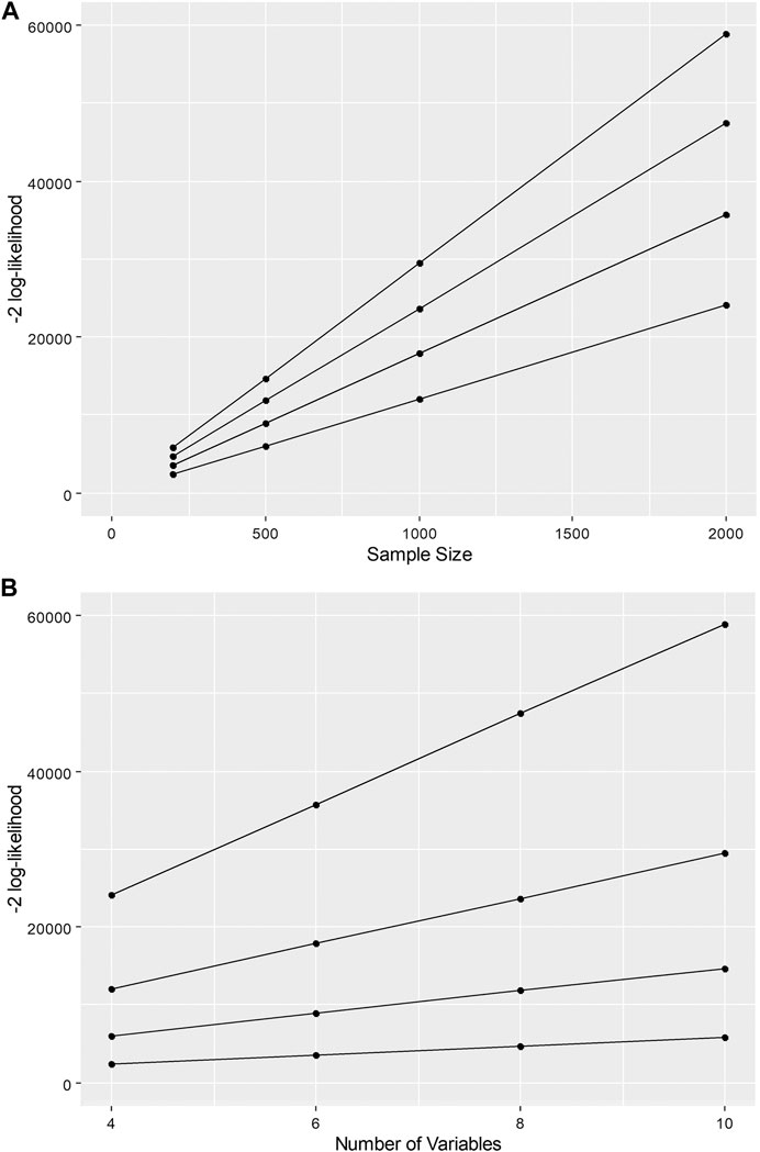
FIGURE 1. −2 log-likelihood as a function of (A) sample size and (B) number of variables in latent profile analysis given a constant difference in a two-class model.
These associations highlight the challenge for information criteria when comparing mixture models. For example, given a constant difference in model fit between two competing models, the difference in the
A second challenge for information criteria is missing data. Specifically, for many information criteria (e.g., BIC,
Approximate likelihood ratio tests have shown tremendous promise in simulation studies and provide a statistical framework for comparing FMMs. We identify two limitations of approximate likelihood ratio tests. The first is that the approximate likelihood ratio tests are only available when comparing FMMs that differ by one class with the same set of model constraints. Thus, the approximate likelihood ratio tests are not available when comparing a 2-class model with a 4-class model, two 2-class models with different constraints, or a 2 and 3-class model with different constraints. The second limitation for the approximate likelihood ratio tests is a limitation shared by all statistical tests, which is the association between the value of the likelihood ratio test and sample size. When working with large sample sizes, the approximate likelihood ratio tests can be significant suggesting the model with more classes fits significantly better than the model with fewer classes even when the difference in model fit is small and meaningless.
The resampling techniques provide important information about the sensitivity of estimating the model’s parameters and the replicability of the model through repeated estimation using bootstrap samples or k-fold cross-validation. This information is not contained in other model fit statistics and is important because FMMs often experience convergence issues. Compared to the other model fit statistics, simulation research on these resampling techniques for FMMs is limited and more research is greatly needed. He and Fan (2019) indicated challenges for the k-fold cross-validation approaches; however, He and Fan (2019) noted that k-fold cross-validation was not strongly related to sample size – a potential plus compared to other model fit criteria.
Given the challenges and limitations of the available model fit criteria, we take an alternative point of view when comparing FMMs. The approach we consider looks at model comparison through the lens of effect sizes to provide context about differences in model fit. In the next section we outline the effect size measure and discuss how it can aid the evaluation of model comparison in FMMs.
An Effect Size Measure for Model Comparison
Effect sizes quantify the magnitude of a parameter or the difference in two entities. For example, Cohen’s d (Cohen, 1988) is an effect size measure when comparing means for two groups of individuals. Cohen’s d is defined as
where
In multiple regression analysis with numeric predictors, the commonly reported effect size is the standardized beta weight. In linear regression, the standardized beta weight is calculated as
where
For determining an effect size measure for model comparison, our goal is to scale the difference in the
where
The main reason to do this is to provide context regarding the relative improvement in model fit. The examination of model comparison indices, such as information criteria, through simulation is focused on recovering the number of classes that are known to exist within the data. Even though researchers control the distinctiveness of the classes, we don’t have an appropriate metric for this distinctiveness. When fit indices fail to uncover the proper number of classes, the blame is put on the fit index. If the same approach were taken in simulation studies for the analysis of variance, we may lead to the conclusion that null hypothesis significance testing (NHST) isn’t working. For example, NHST is unable to consistently find a significant difference between two means when Cohen’s
The second reason for considering the LIP for model comparison is because it should be weakly related to sample size because it is scaled by the
To determine how the LIP changes as a function of different latent class structures and sample sizes, we mimic two previously conducted simulation studies. The first is Nylund et al.'s (2007) simulation study for latent profile analysis and the second is Grimm et al.'s (2013) simulation study for growth mixture models.
LIP Effect Sizes
Latent Profile Models
Simulation research following the population models for latent profile analysis (latent class analysis with continuous indicators) in Nylund et al. (2007) was conducted to examine the LIP. For the LIP, we examined the percent improvement in the
Nylund et al. (2007) examined three latent profile population structures (8-variable simple, 15-variable simple, and 10-variable complex) under three sample sizes (
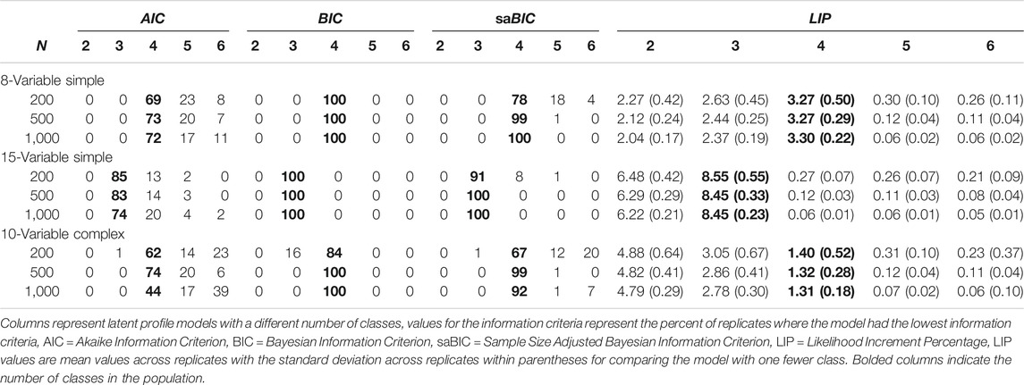
TABLE 1. Model selection in latent profile structures from Nylund et al. (2007) and associated LIP values.
The mean LIP and the standard deviation of LIP values across replicates are contained on the right-hand side of Table 1. The first LPA structure was the 8-variable simple structure population model, which had four classes. The mean LIP comparing the 1 to 2, 2 to 3, and 3 to 4-class models were all over 2; however, the mean LIP comparing the 4- to 5-class model was 0.30 or smaller. For all sample sizes in the 8-variable population structure, there was a clear drop in the LIP after the 4-class model. The LIP values were fairly consistent across sample sizes, as was expected for effect size type measures. In this 8-variable population structure, there were two items for each class with a mean of 2 and all remaining items had means of 0 (with standard deviations of 1) to indicate the distinctiveness of the classes in this simulation condition.
The second population structure was the 15-variable simple structure, where there were three classes in the population. Each class had five variables with a mean of 2 with remaining variables having a mean of 0 (with a standard deviation of 1). Again, there were clear changes in the LIP after the 3-class model. LIP values were greater than six when comparing the 1 to 2-class model and when comparing the 2 to 3-class model. The average LIP was less than 0.30 when comparing the 3 and the 4-class model. Thus, the LIP clearly delineated the population structure. Again, the classes were well separated in this population structure. The higher-values of the LIP, compared to the 8-variable population structure, reflect two things. First, the classes in the 15-variable simple population structure were more distinct. That is, five variables distinguished each class compared to two-variables in the 8-variable simple population structure. Second, the difference in the number of estimated parameters when increasing the number of classes. Specifically, nine parameters were added when increasing the number of classes by one in the 8-variable simple population structure, and 16 parameters were added when increasing the number of classes in the 15-variable simple population structure. This second reason suggests determining the percent improvement in model fit per additional parameter. Dividing LIP values by the difference in the number of additional parameters makes them more comparable. For example, dividing the 4-class LIP values for the 8-variable simple structure by nine yields 0.37, and dividing the 3-class LIP values for the 15-variable simple structure by 16 yields 0.53.
The third and final LPA population structure in Nylund et al. (2007) was the 10-variable complex structure. In this population structure there were four classes, and no one variable distinguished each class. There was a class with a mean of two for all variables, a class with a mean of two for the first five variables and a mean of zero for the second five variables, a class with a mean of zero for the first five variables and a mean of two for the second five variables, and a class with a mean of 0 for all ten variables. Additionally, class sizes were unequal with relative class sizes being 5, 10, 15, and 70% (note Nylund et al. (2007) reports 75% in the fourth class). As with the other two population structures, the mean LIP clearly indicates when more classes were not warranted. The mean LIP was 4.8 when comparing the 2 and 1-class models, 2.9 when comparing the 3 and 2-class models, and 1.4 when comparing the 4 and 3-class models. The comparison of the 5-class model to the 4-class model yielded a mean LIP that was less than 0.4 – a similar value was obtained in the other population structures. The class differences were not as distinct in this third population structure, which is highlighted by the smaller LIP values when moving from the 3-class model to the 4-class model. Dividing the LIP by the difference in the number of estimated parameters yields 0.12. Noticeably smaller than the other two population structures where the class differences were much larger.
Growth Mixture Models
The growth mixture modeling simulations by Grimm et al. (2013) focused on two-class mixture models and varied sample size (
Table 2 contains model selection percentages based on the AIC, BIC, and

TABLE 2. Model Selection in Growth Mixture Modeling Structures with intercept differences, five time points, and 50–50 mixing proportion from Grimm et al. (2013) and Associated LIP values.
In the middle section of Table 2, the intercept means were two standard deviations apart. Here, the
Table 3 contains four more population structures. In all of these population structures, the means of the intercepts were three standard deviations apart. In the first two, the mixing proportion was 80–20 and 95–5, respectively. In Grimm et al. (2013), the 80–20 mixing proportion led to slightly better model selection rates for the information criteria, and the 95–5 mixing proportion led to slightly worse model selection rates compared to when the mixing proportion was 50–50. These patterns held for these simulations. Compared to when there was a 50–50 mixing proportion, the LIP values were slightly greater for the 80–20 mixing proportion (∼0.40) and slightly lower for the 95–5 mixing proportion (∼0.21), which was consistent with the performance of the information criteria.
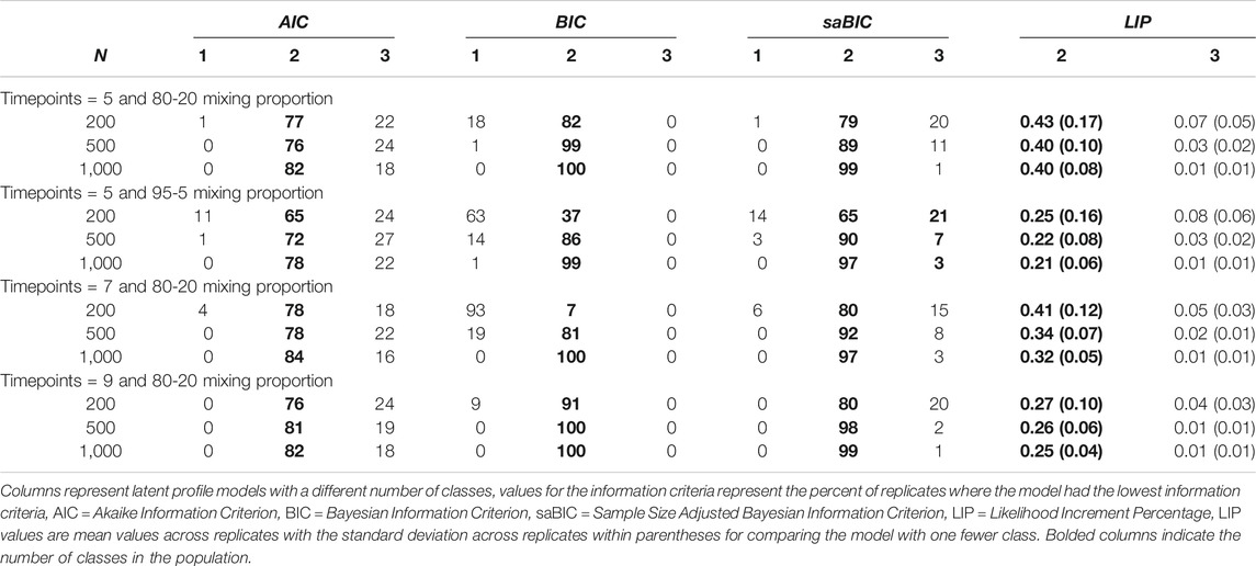
TABLE 3. Model selection in growth mixture modeling structures with a three standard deviation difference in the intercepts from Grimm et al. (2013) and Associated LIP values.
In the second two population structures, the number of measurement occasions was changed to seven and nine, respectively. In these population structures, the intercept means were three standard deviations and the mixing proportions were 80–20. The effect of the number of time points in this population structure was unexpected. The information criteria correctly identified the two-class models slightly more with nine measurement occasions, compared to the five time point data; however, the BIC struggled when there were seven measurement occasions with
Interim Summary
Overall, the LIP showed a clear drop when no more classes were warranted for all of the latent profile models. The drop in the LIP was less clear for the growth mixture models. In the growth mixture models, the distinctiveness of the two classes was varied systematically. The LIP did not show a systematic change after the two-class model when the classes differed by one standard deviation in the intercept mean. There was a small drop when the intercept means were two standard deviations apart, and a clear drop when the intercept means were three standard deviations apart. In the growth mixture modeling simulations, the information criteria performed poorly, which highlights the challenges in comparing FMMs.
Although the performance of the LIP was admirable, there were two concerns. First, the LIP was mildly associated with sample size. That is, the LIP tended to be higher with
LIP Effect Sizes
The performance of the LIP leads to the question of how the LIP should be used for model comparison. We propose first examining how the LIP changes when increasing the number of classes. Ideally, the LIP will drop off when no more classes are warranted – akin to scree plot in factor analysis. Second, we recommend dividing the LIP by the increase in the number of estimated parameters when a class is added to the model. This LIP per parameter (
The
Discussion
Model comparison in FMM is challenging and existing model fit indices, such as information criteria, approximate likelihood ratio tests, and those based on resampling techniques do not provide standardized information about the relative improvement in model fit. The LIP, initially proposed by McArdle et al. (2002) for model comparison, was divided by the difference in the number of estimated parameters and is a proposed effect size to aid model comparison for FMMs. This
When comparing two models, researchers have categorized differences in the AIC (Burnham and Anderson, 2004) and BIC (Kass and Raftery, 1995), and proposed an approximate Bayes Factor, to provide context regarding the magnitude of the difference in model fit. While not the same as an effect size, the contextual comparison is helpful when comparing two (or more) models. The
Mahalanobis Distance and Entropy
There are two important pieces of statistical information from FMMs that are relevant when discussing the LIPpp – Mahalanobis distance (Mahalanobis, 1936) and entropy. Mahalanobis distance is a measure of the distance between two mean vectors standardized by a common or pooled covariance matrix. Mahalanobis distance has been utilized as an effect size measure for the separation of two classes in FMM simulations (Grimm, et al., 2013; Peugh and Fan, 2012, Peugh and Fan, 2015). The multivariate Mahalanobis distance is calculated as
where
Entropy is a measure of classification quality and is calculated as
where
Concluding Remarks
The
Data Availability Statement
The original contributions presented in the study are included in the article/Supplementary Material, further inquiries can be directed to the corresponding author.
Author Contributions
KG developed the idea, conducted simulation work, and drafted the paper. RH conducted the literature, helped draft the introduction, and edited the paper. DR helped draft the introduction and edited the paper.
Conflict of Interest
The authors declare that the research was conducted in the absence of any commercial or financial relationships that could be construed as a potential conflict of interest.
References
Abdolell, M., LeBlanc, M., Stephens, D., and Harrison, R. V. (2002). Binary partitioning for continuous longitudinal data: categorizing a prognostic variable. Stat. Med. 21, 3395–3409. doi:10.1002/sim.1266
Akaike, H. (1973). “Information theory and an extension of the maximum likelihood principle,” in 2nd International symposium on information theory. Editors B. N. Petrov, and F. Csáki (Budapest, Hungary: Akadémiai Kiadó), 267–281.
Burnham, K. P., and Anderson, D. R. (2004). Multimodel inference: understanding AIC and BIC in model selection. Sociol. Methods Res. 33, 261–304. doi:10.1177/0049124104268644
Cohen, J. (1988). Statistical power analysis for the behavioral sciences. 2nd Edn. Hillsdale, NJ: Lawrence Erlbaum Associates Publishers, 567.
Cubaynes, S., Lavergne, C., Marboutin, E., and Gimenez, O. (2012). Assessing individual heterogeneity using model selection criteria: how many mixture components in capture-recapture models?: heterogeneity, mixtures and model selection. Methods Ecol. Evol. 3, 564–573. doi:10.1111/j.2041-210X.2011.00175.x
Fernández, D., and Arnold, R. (2016). Model selection for mixture-based clustering for ordinal data. Aust. N. Z. J. Stat. 58, 437–472. doi:10.1111/anzs.12179
Gibson, W. A. (1959). Three multivariate models: factor analysis, latent structure analysis, and latent profile analysis. Psychometrika 24, 229–252. doi:10.1007/BF02289845
Grimm, K. J., Mazza, G. L., and Davoudzadeh, P. (2017). Model selection in finite mixture models: a k-fold cross-validation approach. Struct. Equ. Model. 24, 246–256. doi:10.1080/10705511.2016.1250638
Grimm, K. J., Ram, N., Shiyko, M. P., and Lo, L. L. (2013). “A simulation study of the ability of growth mixture models to uncover growth heterogeneity,” in Contemporary issues in exploratory data mining. Editors J. J. McArdle, and G. Ritschard (New York, NY: Routledge Press), 172–189.
He, J., and Fan, X. (2019). Evaluating the performance of the k-fold cross-validation approach for model selection in growth mixture modeling. Struct. Equ. Model. 26, 66–79. doi:10.1080/10705511.2018.1500140
Hurvich, C. M., and Tsai, C. L. (1989). Regression and time series model selection in small samples. Biometrika 76, 297–307. doi:10.1093/biomet/76.2.297
Kass, R. E., and Raftery, A. E. (1995). Bayes factors. J. Am. Stat. Assoc. 90, 773–795. doi:10.1080/01621459.1995.10476572
Kass, R. E., and Wasserman, L. (1995). A reference Bayesian test for nested hypotheses and its relationship to the Schwarz criterion. J. Am. Stat. Assoc. 90, 928–934. doi:10.1080/01621459.1995.10476592
Lazarsfeld, P. F. (1950). “The logical and mathematical foundation of latent structure analysis and the interpretation and mathematical foundation of latent structure analysis,” in Measurement and prediction. Editors S. A. Stouffer, L. Guttman, E. A. Suchman, P. F. Lazarsfeld, S. A. Star, and J. A. Clausen (Princeton, NJ: Princeton University Press), 362–472.
Liu, M., and Lin, T. I. (2014). A skew-normal mixture regression model. Educ. Psychol. Meas. 74, 139–162. doi:10.1177/0013164413498603
Lo, Y., Mendell, N. R., and Rubin, D. B. (2001). Testing the number of components in a normal mixture. Biometrika 88, 767–778. doi:10.1093/biomet/88.3.767
Lubke, G. H., and Campbell, I. (2016). Inference based on the best-fitting model can contribute to the replication crisis: assessing model selection uncertainty using a bootstrap approach. Struct. Equ. Model. 23, 479–490. doi:10.1080/10705511.2016.1141355
Lubke, G. H., Campbell, I., McArtor, D., Miller, P., Luningham, J., and van den Berg, S. M. (2017). Assessing model selection uncertainty using a bootstrap approach: an update. Struct. Equ. Model. 24, 230–245. doi:10.1080/10705511.2016.1252265
Lubke, G. H., and Muthén, B. (2005). Investigating population heterogeneity with factor mixture models. Psychol. Methods 10, 21–39. doi:10.1037/1082-989X.10.1.21
Mahalanobis, P. C. (1936). On the generalised distance in statistics. Proc. Natl. Inst. Sci. India. 2, 49–55.
Masyn, K. (2013). “Latent class analysis and finite mixture modeling,” in The Oxford handbook of quantitative methods in psychology. Editor T. D. Little (New York, NY: Oxford University Press), Vol. 2, 551–611.
McArdle, J. J., Ferrer-Caja, E., Hamagami, F., and Woodcock, R. W. (2002). Comparative longitudinal structural analyses of the growth and decline of multiple intellectual abilities over the life span. Dev. Psychol. 38, 115–142. doi:10.1037/0012-1649.38.1.115
McLachlan, G. J. (1987). On bootstrapping the likelihood ratio test statistic for the number of components in a normal mixture. J. R. Stat. Soc. Ser. C 36, 318–324. doi:10.2307/2347790
Muthén, B., and Shedden, K. (1999). Finite mixture modeling with mixture outcomes using the EM algorithm. Biometrics 55, 463–469. doi:10.1111/j.0006-341X.1999.00463.x
Nagin, D. S. (1999). Analyzing developmental trajectories: a semiparametric, group-based approach. Psychol. Methods. 4, 139–157. doi:10.1037/1082-989X.4.2.139
Nylund, K. L., Asparouhov, T., and Muthén, B. O. (2007). Deciding on the number of classes in latent class analysis and growth mixture modeling: a Monte Carlo simulation study. Struct. Equ. Model. 14, 535–569. doi:10.1080/10705510701575396
Paxton, P., Curran, P. J., Bollen, K. A., Kirby, J., and Chen, F. (2001). Monte Carlo experiments: design and implementation. Struct. Equ. Model. 8, 287–312. doi:10.1207/S15328007SEM0802_7
Peugh, J., and Fan, X. (2015). Enumeration index performance in generalized growth mixture models: a Monte Carlo test of Muthén’s (2003) hypothesis. Struct. Equ. Model. 22, 115–131. doi:10.1080/10705511.2014.919823
Peugh, J., and Fan, X. (2012). How well does growth mixture modeling identify heterogeneous growth trajectories? A simulation study examining GMM’s performance characteristics. Struct. Equ. Model. 19, 204–226. doi:10.1080/10705511.2012.659618
Peugh, J., and Fan, X. (2013). Modeling unobserved heterogeneity using latent profile analysis: a Monte Carlo simulation. Struct. Equ. Model. 20, 616–639. doi:10.1080/10705511.2013.824780
Rindskopf, D. (2003). Mixture or homogeneous? Comment on Bauer and Curran (2003). Psychol. Methods. 8, 364–368. doi:10.1037/1082-989X.8.3.364
Sclove, S. L. (1987). Application of model-selection criteria to some problems in multivariate analysis. Psychometrika 52, 333–343. doi:10.1007/BF02294360
Serang, S., Jacobucci, R., Stegmann, G., Brandmaier, A. M., Culianos, D., and Grimm, K. J. (2020). Mplus trees: structural equation model trees using mplus. Struct. Equ. Model. doi:10.1080/10705511.2020.1726179
Steele, R. J., and Raftery, A. E. (2010). “Performance of Bayesian model selection criteria for Gaussian mixture models,” in Frontiers of statistical decision making and Bayesian analysis. Editors M.-H. Chen, D. K. Dey, P. Müller, D. Sun, and K. Ye (New York, NY: Springer), 113–130.
Stegmann, G., Jacobucci, R., Serang, S., and Grimm, K. J. (2018). Recursive partitioning with nonlinear models of change. Multivar. Behav. Res. 53, 559–570. doi:10.1080/00273171.2018.1461602
Tofighi, D., and Enders, C. K. (2008). “Identifying the correct number of classes in growth mixture models,” in Advances in latent variable mixture models. Editors G. R. Hancock, and K. M. Samuelsen (Charlotte, NC: Information Age), 317–341.
Vuong, Q. H. (1989). Likelihood ratio tests for model selection and non-nested hypotheses. Econometrica 57, 307–333. doi:10.2307/1912557
Wang, K., Yau, K. K., and Lee, A. H. (2002). A hierarchical Poisson mixture regression model to analyse maternity length of hospital stay. Stat. Med. 21, 3639–3654. doi:10.1002/sim.1307
Yang, C. C. (2006). Evaluating latent class analysis models in qualitative phenotype identification. Comput. Stat. Data Anal. 50, 1090–1104. doi:10.1016/j.csda.2004.11.004
Keywords: latent class analyses, growth mixture modeling, model comparison, finite mixture model, latent profile analysis
Citation: Grimm KJ, Houpt R and Rodgers D (2021) Model Fit and Comparison in Finite Mixture Models: A Review and a Novel Approach. Front. Educ. 6:613645. doi: 10.3389/feduc.2021.613645
Received: 02 October 2020; Accepted: 20 January 2021;
Published: 04 March 2021.
Edited by:
Katerina M. Marcoulides, University of Minnesota Twin Cities, United StatesReviewed by:
Ren Liu, University of California, Merced, United StatesJam Khojasteh, Oklahoma State University, United States
Copyright © 2021 Grimm, Houpt and Rodgers. This is an open-access article distributed under the terms of the Creative Commons Attribution License (CC BY). The use, distribution or reproduction in other forums is permitted, provided the original author(s) and the copyright owner(s) are credited and that the original publication in this journal is cited, in accordance with accepted academic practice. No use, distribution or reproduction is permitted which does not comply with these terms.
*Correspondence: Kevin J. Grimm, a2pncmltbUBhc3UuZWR1