Supply-driven evolution: Mutation bias and trait-fitness distributions can drive macro-evolutionary dynamics

Many well-documented macro-evolutionary phenomena still challenge current evolutionary theory. Examples include long-term evolutionary trends, major transitions in evolution, conservation of certain biological features such as hox genes, and the episodic creation of new taxa. Here, we present a framework that may explain these phenomena. We do so by introducing a probabilistic relationship between trait value and reproductive fitness. This integration allows mutation bias to become a robust driver of long-term evolutionary trends against environmental bias, in a way that is consistent with all current evolutionary theories. In cases where mutation bias is strong, such as when detrimental mutations are more common than beneficial mutations, a regime called “supply-driven” evolution can arise. This regime can explain the irreversible persistence of higher structural hierarchies, which happens in the major transitions in evolution. We further generalize this result in the long-term dynamics of phenotype spaces. We show how mutations that open new phenotype spaces can become frozen in time. At the same time, new possibilities may be observed as a burst in the creation of new taxa.

1. Introduction

One of the great and unresolved debates in evolutionary theory is the relationship between micro- and macro-evolution. Micro-evolution is commonly defined as evolution within and among populations (Hendry and Kinnison, 2001; Hautmann, 2020). In practice, this usually means the patterns and processes that are described by the modern and powerful theory of population genetics (Templeton, 2021). Macro-evolution, on the other hand, is the pattern and processes that happen in taxa higher than that of species, over geologic time (Hautmann, 2020).

On the one hand, some authors provide excellent arguments for why macro-evolution should be an extension of micro-evolution (Dietrich, 2009), and on the other hand, other authors have articulated why macro-evolution is a separate process that cannot be distilled to micro-evolution (Erwin, 2000). Among the best arguments of the second school of thought are the many macro-evolutionary phenomena that resist micro-evolutionary explanation. These phenomena fall into four classes: the first class describes the long-term evolutionary trends (McShea, 1994). The trends are empirically controversial (Gregory, 2008), but their theoretical possibility remains a persistent question. The second class represents the major evolutionary transitions (Szathmary and Smith, 2000), such as the increase in a structural hierarchy from RNA molecules to prokaryotes and eukaryotes, from single-cell eukaryotes to multi-cellularity, and from solitary individuals to eusociality. The unusual endurance of major transitions in evolution relates them to a third class of phenomena, sometimes described as “generative entrenchment” (Schank and Wimsatt, 1986; Wimsatt, 1986), where developmental events are profoundly conserved over time. One example would be the hox genes, which are partially responsible for the body plan of lineages. Some aspects of these body plans seem to “lock-in” over time: for example, there is no member of the tetrapod class with more than four limbs. Some developmental events in evolution simply matter more than other events, giving evolution the character of historical contingency (Powell, 2009)—a single such event in developmental pathways can alter the entire evolutionary trajectory of the lineage in which it occurs. The fourth class of macro-evolutionary phenomena is proposed by the proponents of punctuated equilibrium, who argue that micro-evolution provides no satisfactory explanation for the repeated bursts of novelty followed by relative quiescence (Gould, 2009).

Overall, there are several types of micro-evolutionary explanations for the macro-evolutionary phenomena we described above. The first type relies on mutation bias in the absence of natural selection, so genetic drift or neutral evolution dominates. One example is the study of Lynch and Conery (2003) and Lynch (2007), who argued that genomes expanded in complexity in eukaryotes because there was an enormous reduction in the effective population size, increasing genetic drift. Another example is McShea's “zero-force” evolutionary law: in the absence of selection, organisms become more complex (McShea, 2005; McShea and Brandon, 2010) because most mutations produce greater complexity. This type of theory gives an important evolutionary role to mutation bias (e.g., Lynch and Hagner, 2015).

The second type explains evolutionary events based on the external environment and why certain features are adaptive. For example, mitochondria are often explained by referring to improved energy efficiency (Szathmáry, 2015) and multicellularity in terms of the improved efficiency that comes with division of labor (Ispolatov et al., 2012). Such explanations can be made more general by directly mapping macro-evolutionary change to features of the environment. For example, Bell (2010) proposes that the environment displays trends at all scales, so traits, being selected for by the environment, also will display trends at all scales. Taken to the extreme, such explanations are suspicious for teleology (Kampourakis, 2020), which argues for an endless improvement in form and function. This most extreme form of adaptive explanation has not received much support, although there are arguments for ever-improving fitness with improved energy generation or improved division of labor (White, 1943, 2016).

The third type of explanation arises out of evo-devo. This explanation notes that some transcription factors become increasingly conserved over time because they are used in many independent developmental processes. Thus, most of the changes in macro-evolution happen through mutations in genetic regulatory regions, rather than their coding sequences (for an excellent review, see Carroll, 2008).

Unfortunately, none of these explanations are satisfactory. The first type of explanation, mutation bias, imposes strict conditions under which they can matter: the role of natural selection must be nearly zero. The second, based on environmental events, is hard to generalize across macro-evolutionary phenomena: even when we see larger patterns, we cannot explain them except by using the environment as a black-box. The question simply moves from biological evolution to environmental change, which is constrained by our limited understanding of how the environment changes over the long term. The third type is incomplete, that is, the micro-evolutionary basis for this evo-devo phenomenon is not yet known. There is no population genetics theory for why some transcription factors become so widely co-opted (for example, Carroll, 2008).

Here, we introduce the theory of “supply-driven” evolution (SDE), a mechanism based on mutation bias operating in the presence of strong natural selection, which can explain all four classes of macro-evolutionary phenomena described above while remaining compatible with existing theories of micro-evolution. SDE integrates the probabilistic nature of the phenotype-fitness relationship with mutation bias to predict the dynamic evolution of phenotypic spaces and the locking-in of phenotypic structures.

From mutation bias to supply-driven macro-evolution

Mutation bias has historically been rejected as a significant force in evolution, starting with Fisher's early models that pitted mutation bias against natural selection. These models showed that when two alleles are in competition with each other, even a small amount of natural selection in favor of one allele easily overwhelms even large amounts of mutation bias in the opposite direction, especially when mutations are rare (Fisher, 1999). These predictions were based on the assumption that both alleles were already available. However, when only some variation is immediately available for selection, mutation bias can be a fundamental driver of evolution because whichever phenotype arrives first gets the first chance at success (Fontana and Buss, 1994; Stoltzfus, 1999, 2006b; Yampolsky and Stoltzfus, 2001; Stoltzfus and Yampolsky, 2009; Schaper and Louis, 2014). When combined with rugged fitness landscapes, mutation bias can have a profound effect on evolutionary trajectories because a population will discover different fitness hills depending on the frequency of different mutations.

At the same time, developmental biology unequivocally demonstrated that there are constraints on the availability of mutations. Many mutations are developmentally impossible. This means that genetic variation is biased (Alberch and Gale, 1985; Arthur, 2002; Müller and Newman, 2003; Hall et al., 2004; Klingenberg, 2005). Theoretical frameworks inspired by quantitative genetics have formalized verbal arguments about mutation bias and experimental observations from developmental biology (Rice, 1990, 1998, 2012; Klingenberg, 2010). These approaches require measuring and making assumptions about the shape of multivariate phenotype landscapes, such as the trait variance-covariance (G) matrix, as well as the fitness landscape over many traits. The complexity of these models makes intuitive insight difficult.

An alternative approach consists of considering the probabilistic nature of the relationship between trait values and fitness: two organisms with the same trait value do not necessarily have the same fitness (Xue et al., 2015). This is because changes in a trait value such as body length can be achieved via different mechanisms, such as increased cell size or cell proliferation (Arthur, 2001). As another example, there are many ways for different organisms to have the same complexity level, no matter how complexity is measured. There is no reason to expect two organisms, having achieved the same body length or complexity level via different means, to have the same fitness. This insight implies that there is a many-to-many mapping between trait and fitness values. Because a given trait value is realizable from different phenotypes, that trait value can be associated with a range of different fitnesses.

Multiple realizability is also realistic at the genetic level. We know that quantitative traits influenced by many loci are ubiquitous and underpins modern theories of quantitative genetics (e.g., Turelli and Barton, 1990). A great variety of genes must contribute to the weight of an animal, for example, even genes we do not usually associate with body weight. These genes might change muscle mass, fat mass, and the size of one's liver or bones, yet all of them will affect body weight. Thus, two organisms with the same body weight can have different genomes, different phenotypes, and different fitnesses.

The flip side of widespread polygenic traits is widespread pleiotropy, such that most genes also influence many traits to some extent. This means that two organisms with the same trait value, but with different underlying genes that affect that trait, will have different values for other traits (such as the example of body weight given earlier), leading to different phenotypes and thus different fitnesses. Polygenic traits and pleiotropy give a plausible genetic basis of why trait values are multiply-realizable.

Once we see how traits are multiply-realizable, we see that there is a many-to-many relationship between trait values and fitness values. This means each trait value can be associated with a distribution of fitness value.

Consider Figure 1. Here, organisms are strings of integers. The trait value (ϕ) we are interested in is the sum of the string of the organism. Clearly, there are different ways to have the same trait value. In the figure, the initial wild type (Figure 1A) has trait value ϕ^* = 0 and some fitness ω^*. These mutants all have the trait value ϕ_m = 1, but they are clearly different organisms and have different fitnesses, which form a fitness distribution (Figure 1B). Let u be the difference between mutant and wildtype trait value, so u = 1 for all mutants shown. Figure 1B shows the distribution of ζ_S(s|u = 1) over s, which is the difference between the mutants and wildtype fitnesses. For example, $s_1={\omega }_{m1}-{\omega }^{*}$. The y-axis represents the density. Higher values on the y-axis for a particular s value mean that mutants with that s value (that is, that particular fitness) are more common, and lower values mean such mutants are less common. Again, all these mutants have the same trait value, but different fitnesses (multiple realizability).

FIGURE 1

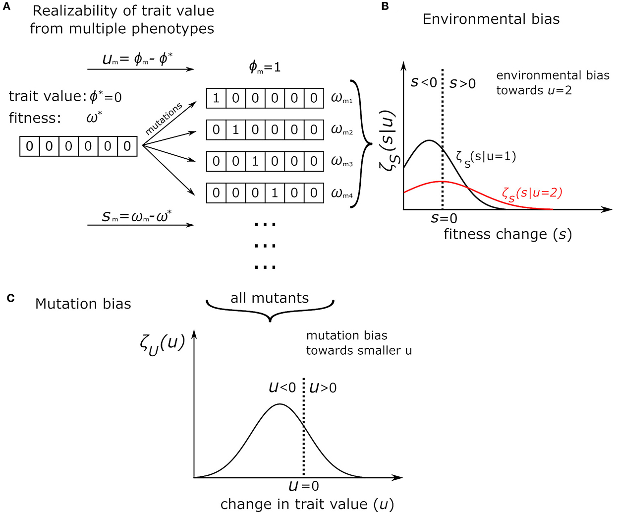
Figure 1. Illustration of multiple-realizability using the NK model. Organisms are strings, the trait value ϕ is the sum of the string. See text for more details. (A) Shows a wild type that mutates into a group of different mutants, all with the same trait value (ϕ_m = 1), but different fitnesses (ω_m). This population of mutants then form a density distribution [ζ, (B)] of fitnesses, with density on the y-axis and $s={\omega }_m-{\omega }^{*}$ (fitness difference from wildtype) on the x-axis. As drawn, mutants with trait value 2 has higher average fitness than mutants with trait value 1 (red line). (C) We have another density distribution, of all possible mutants of the wildtype (rather than all mutants with the same trait value), now over u (the change in trait value) rather than over s. This distribution illustrates mutation bias. As illustrated, there is a mutation bias toward smaller trait value (u < 0).

Consider another mutant population, now with a different trait value (say, u = 2 instead of u = 1). This population may now have a different distribution of fitness values, which would create another density graph (which we draw in red). In this hypothetical case, the environment would favor u = 2, since, on average, the fitness of all mutants with trait value u = 2 is higher than the average fitness of all mutants with trait value u = 1. This is what we mean by environmental bias.

Figure 1C shows another density distribution, but not of fitness. This distribution includes all mutants of the wildtype, not only those with the same trait value. The x-axis now represents different trait values(u), while y-axis represents the density of those trait values. A high y-axis value for a particular u means mutants of that trait value is common, and vice versa. This graph thus represents the distribution of all ζ_U(u). As drawn, it would represent a mutation bias toward smaller u.

The situation described in Figure 1 contrasts with the more common assumption of a one-to-one relationship between trait and fitness. In the common case, mutation bias is a weak driver of evolutionary. In the many-to-many case, however, mutation bias is given much more power: if a particular trait value is created more frequently through mutation bias (Figure 1C), then the possibility of a high fitness variant with that trait value also becomes more likely, because we are sampling more frequently from a distribution of fitness values.

The environment is still accorded an important role (Figure 1B). As in any standard theory of evolution, the fitness value of any particular phenotype is determined by the environment through natural selection. Thus, the fact that the same trait value can be realized by many phenotypes gives us a distribution of fitnesses, but the exact shape of that distribution is determined by the environment. Through natural selection, the environment can still favor certain trait values over others (e.g., the fitness distribution of certain trait values can have a larger mean than the fitness distribution of other trait values), a phenomenon we call environmental bias. We will show that, unlike standard evolutionary theory, this sort of environmental bias does not overwhelm mutation bias.

In this article, we begin by presenting a formal model of supply-driven evolution. We then show how the combination of mutation bias and the trait-fitness distribution can create long-term trends in evolution. Using our framework and simulations of the NK model, we next show how this result implies a special class of evolutionary innovations: those that create new phenotype spaces. We show how supply-driven evolution can cause these innovations to become locked-in over macro-evolutionary time. Our results suggest that the emergence of new phenotype spaces, their locking-in, and their subsequent exploration by micro-evolutionary processes can explain long-term trends in evolution, major evolutionary transitions, generative-entrenchment, and macro-evolutionary burst-quiescence dynamics.

2. Supply-driven evolution: A mathematical framework

Let us consider a homogeneous haploid population with fitness ω^* and a trait with value ϕ^*. Let a mutant m be defined by (s_m, u_m), where s_m = ω_m−ω*, the difference between the mutant and resident fitnesses, and $u_m={\varphi }_m-{\varphi }^{*}$, the difference between their trait values. A mutant-fitness distribution, ζ(s, u), can now be defined over all mutants of the population, which is a bivariate density distribution, the two variables being s and u, that is, the fitness and the trait values. When a mutant enters the population, its fitness and trait values are determined by choosing from ζ. Ordinary evolution then takes place to determine the success of this mutant through genetic drift and natural selection. Note how, in this framework, mutants with the same trait value ϕ_m can have very different fitnesses, drawn from the distribution ζ(s, u = u_m) (see Figure 1).

We will work within a classic adaptationist scenario, where there is a strong selection and a weak mutation (for a categorization of the different regimes of evolution, see Sniegowski and Gerrish, 2010). In this case, mutations are rare and the population is large. When a beneficial one comes along, it can sweep through the population if it escapes drift. In the ideal case, the only driver of evolution in this scenario is selective sweeps, which happen on a timescale that is short compared with the timescale of the generation of beneficial mutants.

We should note that this is the most conservative possible assumption. If we moved our evolutionary regime to one of weaker selection and stronger mutation, such that there are smaller populations or more frequent mutations, then we would expect mutation bias to play an even larger role through processes such as genetic drift or neutral evolution. In fact, the most extant literature on mutation bias depend on these non-selective processes. We are, on the other hand, examining a new mechanism that works even when there is only natural selection. At higher conceptual levels, the basic idea in this paper is that the trait value that succeeds is the trait value that is common, and it does not matter how this success is obtained—through drift or through selection.

To simplify our analytical model, we will further assume that detrimental mutations are evolutionarily inconsequential, that there is no clonal interference (i.e., there is only one adaptive mutation at a time, see Kim and Orr, 2005) and the improvements in fitness are small and incremental. We will see with agent-based models that relaxing these assumptions does not change the final results.

Since improvements in fitness are small, the probability of a mutant with fitness advantage s sweeping the population is αs, where α is a constant that depends on the details of evolution (α = 2 for Poisson distributed offspring Haldane, 1927, α = 1 for a Moran process Nowak, 2006, α≈2.8 for binary fission—see the discussion in Johnson and Gerrish, 2002). Thus, the probability distribution that a mutant will sweep the population and change the trait value by u is a function of u:

$\begin{array}{ll}p(u)\approx \alpha {\displaystyle {\int }_0^{\infty }}s\zeta (s,u)ds& (1)\end{array}$

We integrate over s from 0 to ∞ because we only care about the higher fitness mutants. The probability p(u) does not normalize to 1 over all u, and the probability that there is no selective sweep makes up the rest of the weight.

Of course, ζ(s, u) may change over time, but for now, we will consider a single selective sweep before taking a long-term view. A single selective sweep, under this regime, is rapid.

To simplify this equation and to understand it better, we first can separate out the contribution of mutation bias to evolution. We can split ζ up according to its conditional probability distribution, using the standard notation where U and S are random variables for u and s:

$\begin{array}{ll}\zeta (u,s)={\zeta }_S(s|U=u){\zeta }_U(u)& (2)\end{array}$

Here, ζ_U(u) is the marginal density of mutants that change trait value by u, while ζ_S(s|U = u) is the fitness distribution of all mutants with trait value difference u. In essence, ζ_U(u) is the mutation distribution: it tells us how likely a mutant with particular u is likely to arrive. On the other hand, the environment is captured by ζ_S(s|U = u). For any particular phenotype, its fitness value is determined by the environment. Thus, the exact shape of the distribution of ζ_S(s|U = u) is determined by the environment. The environment can change, leading to changes in the shape of this distribution. For example, if the environment becomes more favorable for a trait value u, the mean of the distribution ζ_S(s|U = u) may increase. Of course, the environment can change ζ_S(s|U = u) in many other ways, such as increase its variance or skew, which can also qualitatively alter evolution.

Next, we split ζ_S(s|U = u) into two parts, the detrimental and the beneficial parts

$\begin{array}{l}{\zeta }_S(s|U=u)=a_u{\zeta }_S(s|U=u,s<0)+b_u{\zeta }_S(s|U=u,s>0)\end{array}$

Where

$\begin{array}{l}{a}_u={\displaystyle {\int }_{-\infty }^0}{\zeta }_S(s|U=u)ds\end{array}$

and

$\begin{array}{l}{b}_u={\displaystyle {\int }_0^{\infty }}{\zeta }_S(s|U=u)ds\end{array}$

That is, a_u is the probability that a mutation that changed the trait value by u is detrimental, and b_u is the probability that a mutation that changed the trait value by u is beneficial. In this case, Equation (1) becomes

$\begin{array}{l}p(u)=\alpha {\displaystyle {\int }_0^{\infty }s}{\zeta }_U(u)b_u{\zeta }_S(s|U=u,s>0)ds\\ =\alpha {\zeta }_U(u)b_u[{\displaystyle {\int }_0^{\infty }s}{\zeta }_S(s|U=u,s>0)ds]\\ =\alpha {\zeta }_U(u)b_u\text{E}[{\zeta }_S(s|U=u,s>0)]\\ ={\zeta }_U(u)\beta (u)& (3)\end{array}$

Here, β(u) = αb_u𝔼[ζ_S(s|U = u, s > 0)] can be called the “degree of benefit” of u, which is the probability that a mutation that changed the trait value by u is beneficial, b_u, multiplied by the size of the expected fitness advantage, 𝔼[ζ_S(s|U = u, s > 0)], multiplied by α. What β measures is the probability that a mutation with trait value u will selectively sweep—that is, the mutation will both be beneficial as well as escape drift. Detrimental mutations drops out of the equation because the integration on s is only from 0 to ∞, that is, in this framework, only beneficial mutations will alter the evolutionary trajectory.

Equation (3) defines the probability that the population trait value will change by u through the introduction of the next mutant. This probability is the product of the likelihood of this mutant appearing, ζ_U(u), the degree of benefit of this change, and a constant factor α. The factor α depends on the exact nature of the evolutionary process as described earlier. In this equation, the mutation distribution plays an equal and symmetric role to environmental selection. A trait value with half the benefit of another trait value can make up for it with double the mutation bias.

We can integrate through all trait values, u, to arrive at the expected change in trait value through the introduction of one mutant:

$\begin{array}{ll}\text{E}\left[u\right]={\displaystyle {\int }_{-\infty }^{\infty }}u{\zeta }_U(u)\beta (u)du& (4)\end{array}$

To recap, the above equation holds in regimes where the only evolutionary events are selective sweeps by beneficial mutations, where beneficial mutations are rare and the fitness effect of beneficial mutations are small. In this formulation, selection affects evolution by changing β(u), while mutation bias is captured by ζ_U(u). The last equation holds for the introduction of a single mutant. As time goes on, both ζ_U and β may change: the former as the structure of the organism changes, thus changing the sort of mutants it produces, and the latter will change as the environment changes.

Prediction of trait change in an agent-based model

We can first apply (Equation 1) to predict how a trait evolves in agent-based simulations where ζ_U(u) and β(u) are known or can be measured. To demonstrate this, we adopt an agent-based model that was previously used to show that mutation bias can direct the evolution of a trait (Stoltzfus, 2006a), even against environment selection (Xue et al., 2015).

The model is an agent-based NK model (Kauffman and Levin, 1987), where agents are strings made from elements of 0's and 1's. There are interactions among these elements that create a rugged fitness landscape. Mutations flip 0's to 1's and vice-versa. The trait we measure is the sum of all the elements. The environmental bias is defined in such a way that the larger this sum, the more likely that the agent is fit. There is a mutation bias in the opposite direction, however, in the sense that mutations from 1 to 0 are more common than mutations from 0 to 1 (Figure 1A, refer to Supplementary Section 1 for details).

In this model, ζ_U is known because it corresponds to how often mutations change 0 to 1 or vice versa. β(u) needs to be measured, because it is a dynamic quality determined by how close the population is to a fitness local optimum. β(u) is affected by many factors: the height of the fitness optimum, the rate of change in the environment, and the mutational load, among other things.

Since β(u) measures the degree of benefit provided by a trait value, it will change with the environment—as a population gets close to the optimum of an environment, β(u) ≈ 0 for all u, since there are much fewer mutants with improved fitness (Fisher, 1999). If the environment changes constantly at a regular pace, however, we can expect β(u) to remain relatively constant over time. This is what happens in this model: with a single measurement of β(u), we can make good predictions for the entire time period (Figure 2). In the first plot, there is mutation bias pushing the trait value down, while in the second plot, there is no mutation bias, so there is only an environmental bias pushing the trait value up. In both plots, β(u) was measured at t = 2e4, giving the model time to find an equilibrium between environmental change and mutation selection. After that, β(u) stayed relatively stable over time, so a single measurement allowed us to make good (although imperfect) predictions over the entire simulation both backward and forward through time. Measuring β(u) at t = 0 was less useful since the population has not settled in an equilibrium with the environment. In these cases, the actual long-term rates and directions of a trait's evolution can be known if we can obtain a measurement for β(u).

FIGURE 2

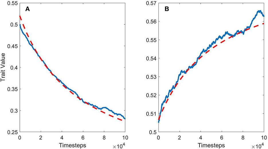
Figure 2. The blue line is the average trait evolution for 200 model runs, the red dashed line is the predicted evolution by Equation (4). For the set of runs in (A), mutation bias pressures the trait value down while the environment is biased to larger trait values. The environment changes over time. (B) Is identical, but without mutation bias, allowing environmental bias to push the trait value upwards.

3. The supply-driven evolution of structural hierarchies

Supply-driven evolution

We will now study scenarios where ζ_U(u) introduces a mutation bias that is unlikely to be reversed by selection from the environment. This means that the behavior of Equation (4) is determined by ζ_U(u), a regime that we call “supply-driven” evolution. This happens when ζ_U(u) satisfies conditions that would guarantee 𝔼[u] > 0 (or, conversely, 𝔼[u] < 0) for almost any β(u). One possible such condition is set below:

$\begin{array}{l}\begin{array}{l}\text{E}\left[u\right]={\displaystyle {\int }_{-\infty }^{\infty }}u{\zeta }_U(u)\beta (u)du\\ ={\displaystyle {\int }_{-\infty }^0}u{\zeta }_U(u)\beta (u)du+{\displaystyle {\int }_0^{\infty }}u{\zeta }_U(u,t)\beta (u,t)du\\ \ge {\beta }_{max}^{-}{\displaystyle {\int }_{-\infty }^0}u{\zeta }_U(u)du+{\beta }_{min}^{+}{\displaystyle {\int }_0^{\infty }}u{\zeta }_U(u)du\end{array}\end{array}$

In the above equation, ${\beta }_{max}^{-}$ is the maximum value of β(u) for all u < 0 and ${\beta }_{min}^{+}$ is the minimum value of β(u) for all u>0.

Thus, 𝔼[u] ≥ 0 if (but not only if):

$\begin{array}{ll}-\frac{{\int }_0^{\infty }u{\zeta }_U(u)du}{{\int }_{-\infty }^{0}u{\zeta }_U(u)du}\ge \frac{{\beta }_{max}^{-}}{{\beta }_{min}^{+}}& (5)\end{array}$

This is actually a very stringent condition. In particular, this condition is hard to satisfy if ${\beta }_{min}^{+}$ is zero or very small. We can sharpen this condition by trimming out a range of u as follows:

Let v be the set of positive real numbers such that β(v) < ϵ, ∀ v ∈ v. Let us define the set v^c as the complement of v, that is, the set of all positive real numbers with v removed. Then, we can guarantee 𝔼[u] ≥ 0 if

$\begin{array}{ll}-\frac{{\int }_{{\text{v}}^{\text{c}}}u{\zeta }_U(u)du}{{\int }_{-\infty }^{0}u{\zeta }_U(u)du}\ge \frac{{\beta }_{max}^{-}}{{\beta }_{min}^{{\text{v}}^{\text{c}}}}& (6)\end{array}$

In the above equation, ${\beta }_{min}^{{\text{v}}^{\text{c}}}$ is the minimum value of β(u) over the set v. This guarantees that ${\beta }_{min}^{{\text{v}}^{\text{c}}}\ge ϵ$, but reduces the value of the numerator on the left side. This is a useful condition, for example, if β(u) drops off to zero for all u larger than some threshold, u_c. This can happen when the environment poses a hard limit to what values u can take, such that all organisms with u > u_c die, rendering β_min for this range to be zero. In that case, in the above equation, v^c reduces to [0, u_c]. Mutation bias can still drive the evolution up to near u_c, so long as ${\int }_{{\text{v}}^{\text{c}}}u{\zeta }_U(u)du$ is large enough.

Supply-driven evolution happens if the above conditions are satisfied over a long period of time. This means that the portion of ζ spread over u > 0 strongly outweighs the portion of ζ spread over u < 0, to the point where it outweighs any likely behavior of β, and this fact remains stable over time. If this is true, then mutation bias dominates the direction of the evolution of u, regardless of the environment.

Biologically, it is easy to see what β_max means. This is the degree of benefit of the optimal trait value over u < 0. Empirically, there are few mutations that would, say, immediately double the ancestor's fitness, no matter what the new trait value is, so β_max is likely to be quite small, certainly < 2. On the other hand, β_min is a biologically important parameter that we have never measured empirically. If β_min is too small, no mutation bias can drive evolutionary trends. We expect β_min to decrease with increasing strength of selection on the trait u compared to selection on the phenotypic realization of that trait. If the environment is directly selecting for body size, for example, with no or weak selection on how body size is phenotypically realized, then β_min will be small or zero for anything other than trait values that drive the lineage closer to optimal body size, and the environment alone is the driver of evolution. If, however, what really matters is the phenotype beneath the trait value, as might be the case for complexity, then β could be relatively independent of u, such that β_min ≈ β_max. In this case, even small amounts of mutation bias can give rise to supply-driven evolution.

The origin of increase in structural hierarchies

The evolution of structural hierarchies captures major transitions in evolution (Szathmary and Smith, 2000) including the transition from the RNA world (Orgel, 2003) to the first cells, from prokaryotes to eukaryotes (Lang et al., 1999), from unicellular to multicellular eukaryotes (Bonner, 1998), and from multicellular organisms to eusociality, such as ants or naked mole-rats, and perhaps humans (Wilson and Hölldobler, 2005). What is most interesting about these major transitions is their durability. As far as we know, among the animal and plant kingdoms at least, there is no free-living unicellular organism that had an obligate multicellular organism as its ancestor. Nearly all animals get cancer, but no cancer cell is known to survive independently of the host other than in highly controlled lab conditions. At the very limit, there are cancers in dogs, clams, and Tasmanian Devils that can infectiously spread, but even they are not known to live autonomously (McCallum, 2008; Metzger et al., 2015).

There are exceptions to this irreversibility. The fungal kingdom has lost multicellularity multiple times to form the modern yeasts (Nagy, 2022); there are solitary organisms that had eusocial ancestors (Wcislo and Danforth, 1997) and there are eukaryotes that have lost their mitochondria (Clark and Roger, 1995; Tovar et al., 1999, 2003; Horner and Embley, 2001; Tachezy et al., 2001; Hampl and Simpson, 2007). In many of these cases, the hierarchy was lost early on: in primitive eusociality (Danforth et al., 2003) or rudimentary multicellularity (Nguyen et al., 2017). The loss of mitochondria is less of a case of secondary loss of a hierarchy as an extreme case of dependency. This case corresponds to the evolution of a more derived version where the mitochondrial genome was fully absorbed and where the mitochondria evolved other functions.

Although there have been explanations for the origin of particular increases in the hierarchy, we note that there is no consensus on a fitness-based theory for why the increase in the hierarchy should persist. Prokaryotes are, by almost any measure, the most successful kingdom on the planet. The main other type of explanation is the drift for the fixation of deleterious alleles in each of the component organisms (Moran, 2003), rendering the hierarchy obligatory. In the next section, we show how this will occur with high probability even when there is no neutral or deleterious drift to fixation and only selection takes place.

The mutation bias that drives the locking-in of hierarchies

When two component organisms live in such close synchrony that they form one unit of selection, that is, they share a measure of fitness and mutations in each affect this joint fitness, then mutations on either components have two effects: one on the fitness of the joint ensemble and another on the fitness of individual components, should they separate from the whole. To see how the separation of the component organisms becomes impossible, we simply have to show a scenario of how the fitness of each component would steadily degrade over time. Components may begin as autonomous organisms, but become fully dependent on the whole over time and unlikely to have a viable fitness when severed from the whole.

We first define the fitness of the component organism as a trait with value ϕ. We assume that mutation bias leads to more frequent detrimental mutations compared to beneficial mutations (Eyre-Walker et al., 2006; Eyre-Walker and Keightley, 2007; Monroe et al., 2022). We then define ω as the fitness of the joint ensemble. We now have u = Δϕ being the change in fitness of the components, should they become separated, while s = Δω is the change in fitness of the joint ensemble, on which selection is immediately acting on.

Since the trait variation u is also a change in the fitness of individual components, we can use Fisher's framework (refer to, e.g., Orr, 2006) considering organisms to be pointed in a high-dimensional space, where each dimension represents a trait. Mutations occur within a mutational volume around the organism and the environmental optimum is another point in this space. Using this framework, theory and experiments both show that detrimental mutations always outnumber beneficial ones. This relation become stronger as the organism approaches the environment optimum (Eyre-Walker et al., 2006).

Assuming this inequality between detrimental and beneficial mutations and its relationship with the environmental optimum, we have:

$\begin{array}{l}{\displaystyle {\int }_{-1}^0}\zeta (S=s,u)du\gg {\displaystyle {\int }_0^{\infty }}\zeta (S=s,u)du\end{array}$

as we approach the environmental optimum. Since u is a change in fitness, its range is [−1, ∞].

However, this implies that

$\begin{array}{l}{\displaystyle {\int }_{-\infty }^{\infty }}{\displaystyle {\int }_{-1}^0}\zeta (s,u)duds\gg {\displaystyle {\int }_{-\infty }^{\infty }}{\displaystyle {\int }_0^{\infty }}\zeta (s,u)duds\end{array}$

Switching the order of integration,

$\begin{array}{ll}{\displaystyle {\int }_{-1}^0}{\zeta }_U(u)du\gg {\displaystyle {\int }_0^{\infty }}{\zeta }_U(u)du& (7)\end{array}$

From this, our aim is to show that 𝔼[p(u)] < 0, that is, we expect the fitness of the component organisms to degrade at each selective sweep, such that over time, they can no longer live autonomously.

In order to achieve this, we must define the relationship between trait and fitness variations. It has first been shown that the magnitude of detrimental mutations among the component organisms are, on average, larger than the magnitude of beneficial mutations (Eyre-Walker and Keightley, 2007). That is, the average detrimental mutation being more detrimental than the average beneficial mutation is beneficial, even if detrimental mutations have a lower bound of −1 while beneficial mutations have no upper bound. This relationship means that:

$\begin{array}{l}-\text{E}\left[{\zeta }_U(u|u<0)\right]>\text{E}\left[{\zeta }_U(u|u>0)\right]\end{array}$

Since

$\begin{array}{ll}\text{E}\left[{\zeta }_U(u|u<0)\right]=\frac{{\int }_{-1}^{0}u{\zeta }_U(u)du}{{\int }_{-1}^0{\zeta }_U(u)du}& (8)\end{array}$

Similarly for 𝔼[ζ_U(u|u>0)], multiplying the Equations (7) and (8) gives us

$\begin{array}{ll}{\displaystyle {\int }_{-1}^0}u{\zeta }_U(u)du\gg {\displaystyle {\int }_0^{\infty }}u{\zeta }_U(u)du& (9)\end{array}$

Since detrimental mutations are always more common than beneficial ones, the above equation is true over time. Thus, we are within striking distance of being in the regime of supply-driven evolution, as we described in the previous section in Equation (5). What matters are the values of β, especially ${\beta }_{min}^{-}$. Biologically, ${\beta }_{min}^{-}$ is asking a deep question: is it likely that mutations that decrease the fitness of a component organism still are beneficial for the joint organism? If the answer is never, then ${\beta }_{min}^{-}=0$ and supply-driven evolution is impossible. However, if it is yes, then ${\beta }_{min}^{-}$ will be a reasonable value, and we may be in the regime of supply-driven evolution, such that

$\begin{array}{ll}\frac{{\int }_{-1}^{0}u{\zeta }_U(u)du}{{\int }_0^{\infty }u{\zeta }_U(u)du}\ge \frac{{\beta }_{max}^{+}}{{\beta }_{min}^{-}}& (10)\end{array}$

In this case, mutation bias will steadily drive u down to 0 regardless of what the environment does. This means that, over evolutionary time, the component organism will no longer be able to separate from the joint organism, as its independent fitness become negligible.

Evolutionary lock-in: An agent-based model

We apply the above theory to an NK model, so agents are strings made from elements of 1's and 0's that interact with each other. However, mutations do not change the elements; instead, they change interactions. Each mutation causes a number of elements to interact with different elements than before. We also have a rarer class of mutations: occasionally, an agent will be joined with another agent, to form a much longer string. We call this a joining mutation. Initially, the elements of the two agents have only a few links with each other, but with mutations, they eventually can be more heavily linked to each other. Finally, long agents can also be cleaved in half to form two individual agents. The interactions that were present between the elements of the two agents when they were a single organism will then be lost.

The environment is constructed such that the longer the agent, the less likely it is to be fit. This is a conservative assumption to show that joining mutations can be locked-in even when the environment is biased against it. There is a 2% penalty to fitness each time the length of the organism doubles. Increasing this penalty increases the amount of time before evolutionary lock-in holds; the system simply has to wait for a joining mutation that increases the fitness for the resulting joined organism, despite its increased length. This is possible because there are different ways for agents to join together, some of which cause an increase in fitness that can overcome the 2% penalty. For details on the model, see Supplementary Section 2.

The time series of organism length over multiple simulations (Figure 3A) illustrates how many joining mutations quickly reverse themselves, but some persist. This persistence means that the number of hierarchies rises over time, despite an explicit fitness penalty for doing so. Focusing on a single simulation where locking-in is observed (Figure 3B), we can show that the increased hierarchy becomes irreversible when two components become increasingly enmeshed with each other as measured by the number of links between the first and second halves of the joint organism (Figure 3C). This is a measure of how much effect a cleaving mutation will have on the organism. This steadily increases with time, which means that a cleaving mutation will have an increasing effect on phenotype over time, reducing its chances of being beneficial. On the other hand, u, the fitness of the component organisms, steadily declines over time (Figures 3D–F). We can see how the component organisms are becoming less and less fit and how much more frequent detrimental mutations are, compared to beneficial mutations (Figure 3G), providing a direct comparison with Equation (7). We can see a spike in the number of mutations that lead to no change in fitness of the whole organism (Figure 3G), which are all the neutral mutations (0.36%), but there are many more detrimental mutations (92.7%) than beneficial mutations (6.94%).

FIGURE 3

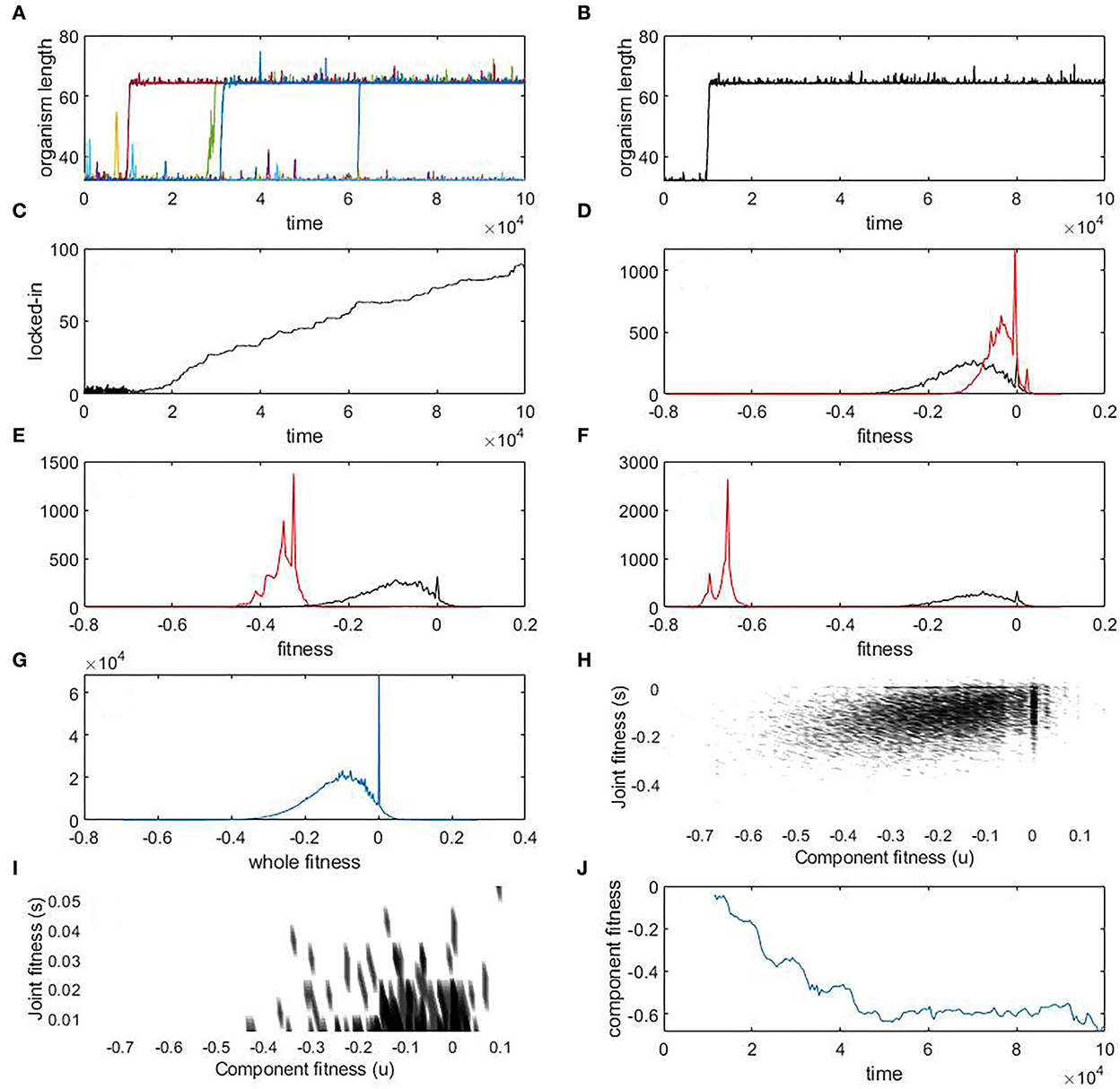
Figure 3. Results from NK simulations. (A) Time series of organism length for eight simulations. (B–J) Results from a single simulation where locking-in of a joining mutation happens early on. See text for more details. For panels (D–G), the y-axis represents the frequency of the distributions. See text for more details.

In this experiment, we can also directly measure ζ(s, u) right after the joining event and directly see that there is a large class of mutations that benefit the larger agent while being detrimental to the component agents (Figures 3H, I). This shows the mutation bias that drives the enmeshment: most mutations that are beneficial to the whole organism are detrimental to the component agent. As these mutations become fixed, the fitness of the component agents, u, steadily declines over time (Figure 3J). These results are compatible with our earlier prediction that due to the strength of the mutation bias, which may be over an order of magnitude in one direction vs. the other, no naturally observed level of selection is likely to reverse this decline in fitness of the component organisms.

4. Generalized evolutionary lock-in

We now generalize this mechanism to a theory of evolutionary lock-in beyond the specific case of joining mutations. In the above example, joining mutations become irreversible (i.e., lock-in) because they create a phenotypic space that was not previously possible—the joint organisms. If this new space is large enough, then supply-driven evolution will push the trajectory of the lineage into the new space, since there will be many more mutations that link the two organisms together than mutations that separate them. Once the lineage has remained in this new phenotypic space (the joint organism) for a while, returning to the old space becomes impossible because component organisms have had their fitnesses degraded beyond return.

We now generalize this example by defining σ as a “potentiation” structure (Blount et al., 2012). This is a structure that creates new phenotypic possibilities. To be specific, σ makes N new mutations possible, and if σ is lost, then these N mutations become impossible again. We assume that this mutation space is unstructured, meaning that the N mutations are independent of each other. σ becomes locked-in when mutations that cause σ to be lost become almost certainly detrimental. This means a very long time must pass before σ is lost. If this time is long compared to the duration of the lineage, then the lineage is more likely to become extinct than to lose σ.

We now show that σ's lifespan scales exponentially in N (to the order of Ω(a^N), where a is a constant larger than 1), so that even for moderately large values of N, σ can lock-in (i.e., remain conserved for such a long period of time that the lineage is most likely to end before σ is lost). Immediately after σ is gained, we track the number of new mutations n, made possible by σ, which become real. Clearly, n will vary from initially 0 to a maximum of N. At each selective sweep, the organism can either gain or lose such a mutation, so n can either increase or decrease. We do not track the selective sweeps that neither produce a gain nor a loss of a mutation in this space because such selective sweeps do not change the ultimate outcome in this system. In addition, there is a certain number of mutations, B, that cause σ to be lost. If σ is lost, all n of the newly realized mutations are also lost. In the previous NK model, there is only one such mutation (so, B = 1), the cleaving mutation that split the joint organism back into two, and all the interactions between the two are lost.

Our task is to show that, for these B mutations that cause σ to be lost, the probability that they sweep the population becomes vanishing small over time. Let us say that, if n = 0 (that is, no new mutations were lost), then the class of all mutations that cause the loss of σ has benefit β, where the benefit is defined as in Equation (3): the probability that this class of mutations has of sweeping (both being advantageous and escaping drift). In the NK model, this would be the likelihood that a cleaving mutation sweeps the population if there were no links between the first and second halves of the joint organism.

We re-emphasize that, when σ is lost, all the mutations that were gained in the new mutation space are lost. The more mutations that are lost, the less likely that the loss of σ would be beneficial. If n new mutations were lost, we assume that the probability that the reversal mutation is advantageous is μⁿ for some 0 < μ < 1. We justify this as follows: lets say that for the n mutations lost, each lost mutation has a probability ν of being advantageous. Conservatively, lets say that having more than n/2 of the mutations lost must be advantageous for the mutation that reverses σ to be, overall, advantageous. (The choice of n/2 is arbitrary, any fraction would work—we would just make a variable substitution in n.) This corresponds to the cumulative binomial density function, Pr(B(n, 1 − ν) ≥ ⌊n/2⌋). Since ν is the probability of an advantageous mutation, we can reasonably assume that 1 − ν > 1/2, which means that Hoeffding's inequality holds:

$\begin{array}{l}\text{Pr}(B(n,1-\nu )\le \lfloor n/2\rfloor )\le exp\left(-2n{\left(\nu -\frac{1}{2}\right)}^2\right)\end{array}$

The probability that a mutation that reverses σ is beneficial is at most μⁿ, where

$\begin{array}{l}\mu =exp\left(-2{\left(\nu -\frac{1}{2}\right)}^2\right)\end{array}$

Thus, the probability that a mutant which lost σ can sweep the population is simply βμⁿ.

At time t, let there be n(t) new mutations that have been actualized. At this point, there are n new mutations that can be lost and N−n new mutations that can be gained. If all mutations have the same probability, this corresponds to the strength of the mutation bias that will increase or decrease n(t). Initially, there are N mutations that will increase n(t) and 0 that will decrease it, leading to a very strong mutation bias. At n = N/2, there will be equal numbers of mutations that increase or decrease n(t), so there will be no more mutation bias that favors the increase of n(t).

There can, of course, be an environmental side to this, such that increases or decreases in n(t) can be favored or disfavored by the environment. However, this will be unimportant in our case for even moderately large values of N, since at the beginning of the process of exploring the new mutation space, n will be very small and so N ≫ n, a difference that will be very hard for the environment to overcome. By the intuition we have developed in this article, we can see that although the environment can alter the specific values of equilibrium n(t), it is unlikely to alter the ultimate outcome of whether σ can be locked-in.

In this case, let us assume that the fitness benefit of increasing n is p, and of decreasing n is q. The benefit of a mutation that reverses σ is β. With these notations, we can now model the system with the Markov chain transition matrix, S, of size N+2:

$\begin{array}{ll}\text{S}=\left[\begin{array}{cccccc}0& \frac{Np}{D_0}& ...& ...& ...& \frac{B\beta }{D_0}\\ \frac{q}{D_1}& 0& \frac{(N-1)p}{D_1}& ...& ...& \frac{B\beta \mu }{D_1}\\ 0& \frac{2q}{D_2}& 0& \frac{(N-2)p}{D_2}& ...& \frac{B\beta {\mu }^2}{D_2}\\ ·& ·& ·& ·& ·& ·\\ ·& ·& ·& ·& ·& ·\\ ·& ·& ·& ·& ·& ·\\ 0& ...& \frac{(N-1)q}{D_{N-1}}& 0& \frac{p}{D_{N-1}}& \frac{B\beta {\mu }^{N-1}}{D_{N-1}}\\ 0& ...& ...& \frac{Nq}{D_N}& 0& \frac{B\beta {\mu }^N}{D_N}\\ 0& ...& ...& ...& 0& 1\end{array}\right]& (11)\end{array}$

Here $D_i=(N-i)p+iq+B\beta {\mu }^i$.

We can show that the expected time to losing σ, or T_B, for p = q = β and B = 1, is (refer to Supplementary Section 3).

$\begin{array}{ll}\text{E}\left[T_B\right]=\Omega {\left(\frac{2}{1+\mu }\right)}^N& (12)\end{array}$

Thus, for this parameter range, once a potentiation structure comes about, the expected time before it is lost increases exponentially with its amount of phenotypic novelty.

We should also note that this process does not only involves the opening of new phenotypic spaces by the introduction of σ but also closes off old phenotypic spaces, because all the mutations that cause σ to be lost (there are B of them) are now rendered evolutionarily impossible. There is, thus, an opening, but also a closing of evolutionary space over time. This mechanism works generally: all evolutionary innovations that open sufficiently large new phenotypic space can become locked-in. σ can represent the formation of eukaryotes, multicellularism, or eusociality, and it can also be associated with new ways of patterning that are not necessarily hierarchical, such as the formation of body axes or of limbs.

Discussion

Evolutionary biologists have long had an intuition that macro-evolution is a different kind of process from micro-evolution (Vrba, 1984; Gould, 1994; Eldredge et al., 2005; Jablonski, 2008; McShea and Brandon, 2010). This intuition has been criticized from the view that macro-evolution is “nothing but” successive rounds of micro-evolution. Balanced against the latter view, some see evolutionary biology to be an essentially historical science (Gould, 1989; Beatty, 1995, 2008), contingent upon historically significant events such as major evolutionary transitions (Szathmary and Smith, 2000; Szathmáry et al., 2011). These problems still resist standard explanations of modern theory. The mechanism presented here may answer some of these problems. We explain these macro-evolutionary phenomena in a way that is compatible with micro-evolutionary processes with an evolutionary regime called “supply-driven evolution” (SDE). In SDE, micro-evolution drives macro-evolution via natural selection, but mutation bias changes the phenotypes that are present for natural selection. We show that this process can dynamically open or close phenotypic spaces. Our analysis and simulation results show how SDE provides an appropriate framework to study long-term evolutionary trends, some of the major transitions in evolution, the profound conservation (locking-in) of certain structures, as well as the episodic creation of new taxa.

Our framework describes macro-evolutionary patterns where micro-evolutionary changes come about primarily by the selective sweep of rare beneficial mutations. The next, and most important, requirement is that a given trait value must correspond to a phenotypic space that includes many different phenotypes, each with their own fitness, and collectively resulting in the distribution of fitness for any given trait value. For example, two very different organisms can have the same height or weight. Second, we assume a distribution of mutation probabilities allowing for a bias in the order of introduction of mutants. If a particular trait value is introduced more frequently, then one of its associated phenotypes is more likely to succeed.

Applying selective sweeps to these fitness and mutation distributions, we show how there are scenarios where mutation bias can be so strong that no environment is likely to reverse it. We called these regimes “supply-driven” evolution (SDE). The most obvious use for SDE is to show how mutation bias can create long-term evolutionary trends. However, it can also show how the major evolutionary transition resulting from increases in structural hierarchies become irreversible, from self-replicating RNA molecules to prokaryotes, to eukaryotes, to multicellularity, and to eusociality. Mutations that lead to such hierarchies are those that join organisms into a new joint organism. We showed that these mutations create new phenotypic space as the new joint organism. This space defines traits with their respective fitness distributions. One such trait is the likelihood of breaking the joint organism into its components, which requires components to be more fit than the joint organism. This trait is part of a phenotypic space created along with the joint organism and is realizable in many different phenotypes. We showed that a strong mutation bias drives this likelihood down over time because most of the mutations that benefit the joint organism will be detrimental to the component organisms.

We then showed that this mechanism generalizes to any structure that makes possible new phenotypes. If a new structure came about that makes available a new set of possible phenotypes that were not previously evolutionarily accessible, then we showed that this structure can be evolutionarily locked-in over time such that no descendant of the lineage of this organism will break it. The measure we consider is the likelihood that this structure will break in a way that is selectively favorable; but there is a strong mutation bias driving this likelihood lower over time. The bias is because there are, at least initially, many more ways to enter into the new set of possibilities than to leave it, and once enough new possibilities are realized, breaking the structure that made it all possible is almost certainly detrimental. The new structure thus opens new space, but closes off old ones.

The theory of SDE expands macro-evolutionary theories beyond the Modern Synthesis, while not rejecting any of its elements. The fact that eukaryotism has persisted might have nothing to do with whether it is evolutionarily advantageous for the lineage (except for that short moment in which it came about); but rather because eukaryotism was impossible before and possible afterward. Once a large enough swathe of novelty becomes possible, SDE shows that there is a chance the structure behind the novelty becomes necessary. SDE also contributes to reconciling the role of structures with the Modern Synthesis (Gould, 1994). After all, what determines the innovations produced by mutations is simply the existing structures within organisms. For example, exaptation has a natural home in SDE: a structure that creates a new space of possibility is also creating a new role for itself. Feathers, for example, originally selected for temperature homeostasis, also create a new space of possibility, which includes flight and, from there, the entire evolutionary space of birds, which were impossible before feathers (Foth et al., 2014). SDE shows that when such a new space is created, the innovation locks-in and its continued existence becomes divorced from the original reason the innovation was selected for.

Another important phenomenon can be made sense of in the light of this theory: the empirical insight that the most evolutionarily impactful innovations are actually quite silent in the moment of their invention (Erwin, 2021), as their immediate effects may be small. There is evidence, for example, that a long period of cryptic evolution has been present before the Cambrian explosion (Zhang and Shu, 2021). Closer to home, this phenonmenon was seen in the Long Term Evolution Experiment (LTEE) when aerobic citrate utilization evolved among lineages of E. coli (Blount et al., 2008, 2012, 2018; Wiser et al., 2013). This ability to use citrate requires several prior mutations, or “potentiation,” before it can be “actualized” by later mutations (Blount et al., 2012). Our study shows that a potentiation structure, if it opens a large enough space, will likely lock-in and form a part of historical contingency (Blount et al., 2018). However, Blount et al.'s work also shows the current experimental challenges to SDE: potentiation structures can be evolutionarily very quiet: that is, their immediate ecological effect could be very hard to detect. Whatever the size of the space they have opened up, that space remains silent until the actualization, and observers only see the actualization.

The macro-evolutionary impact of an evolutionary change is not the ecological effect it has at the moment, but the size of the novel evolutionary space the lineage gains. A large space “sucks” the lineage into it, and its future ecological effects take place inside the new set of possibilities. In this way, the opening of new evolutionary space becomes the macro-evolutionary equivalent of fitness; a new structure that opens new evolutionary space has a probability of “locking-in,” in the same way that a mutation that increases fitness has a probability of sweeping. This is happening even when all that observers can see are selective sweeps of populations through differences in fitness. What the observer cannot observe, however, are the enormous spaces of mere potential that might be opening or closing at each selective sweep. On the other hand, these invisible spaces exert a real evolutionary force, metaphorically similar to a vacuum, because a large potential space will “suck in” evolutionary trajectories. Such a large space forms the underlying and invisible universe of the possible from which the actual and observed are chosen. Their appearance, and the subsequent entry of the lineage into that new space, could be observed as punctuated equilibrium: the sudden creation of new taxa, composed of phenotypes that were previously impossible.

Another theory that shares a theme with SDE is that of constructive neutral evolution (CNE) (Force et al., 1999; Stoltzfus, 1999; Doolittle, 2012; Muñoz-Gómez et al., 2021). In CNE, evolutionary events can create “excess capacity,” which means relaxing certain selective constraints and allowing previously forbidden change (Stoltzfus, 1999; Muñoz-Gómez et al., 2021). That is, this excess capacity means that a range of previously detrimental mutations are now neutral, and therefore possible. These neutral mutations are then introduced into the population at frequencies dictated by mutation bias, leading to ever-increasing complexity.

One canonical and easy to understand example of CNE is the duplication of genes (Brunet and Doolittle, 2018). Once a gene is duplicated, excess capacity is created, because loss-of-function mutations in either of the duplicates, previously detrimental, are now rendered neutral. Due to mutation bias, loss-of-function mutations in either of the duplicate genes are common, and being neutral, they can spread through the population. After this process, the new duplicate gene can no longer be lost, since each of the duplicates suffered different loss-of-function mutations, leading to a rise in organism complexity.

We have sought to demonstrate that SDE can apply even under conditions where neutral evolution and CNE are not operating: the strong-selection and weak mutation regime where the observer can only see natural selection at work. The insight SDE makes is that the fittest organism is more likely to occur in the trait space that is the most common, and hence the trait space that occurs most frequently is also the space that will dominate, even if there is only natural selection. There is, thus, nothing neutral about SDE. The consequence of SDE is that even if one only sees natural selection at work, one still has to assess the space from which mutations are being sourced (the supply of evolution) in order to determine the direction of evolution and cannot assume that such direction will be driven by environmental demands (the demand of evolution).

When SDE is applied to evolutionary locking-in, then both SDE and CNE are explanations of the same phenomenon: why evolution moves into phenotypic spaces favored by entropy (as expressed by mutation bias) rather than natural selection. However, they are quite different explanations. CNE requires excess capacity to render a large field of mutations neutral, then uses neutral evolution to move into the high entropy space. SDE simply makes the insight that high-fitness organisms already are most likely in the high entropy space.

In evolutionary lock-in, SDE requires that new potential structures be made possible. After that, because mutation bias moves evolution into the new potential space, the fittest organism will also be found inside the new potential space. Once this potential space is filled, the original structure that makes it possible can no longer be lost.

The new potential described by SDE is different from excess capacity as defined by CNE. Consider another hypothetical SDE example: early in the origin of metazoans, hox genes came about, allowing for body segmentation and head–tail differentiation. In this case, similar to the origin of eukaryotes, wholly new possibilities came about, and SDE predicts that the highly fit phenotypes, regardless of the environment, are likely to be in the set of new possibilities. These new possibilities were not previously detrimental or forbidden mutations that are newly rendered neutral by some excess capacity; they are simply new. For evolutionary lock-in to happen, SDE merely needs the creation of a large pool of new possibilities; whether those possibilities are detrimental, neutral, or adaptive is not as important as the size of that pool. SDE asserts that, given a large enough pool, there will be some adaptive phenotypes in there, and if a pool is large enough, the next successful phenotype will come from that pool.

There are a plethora of future directions. For example, we have asserted the existence of mutations that makes new evolutionary space possible. This is equivalent to assuming a certain topology of permissible evolutionary space, one that resembles a tree—such that a particular direction opens new fields and closes old ones. This type of topology was hypothesized to drive “epochal evolution” (sensu Crutchfield and Nimwegen, 2002; Crutchfield, 2003) and was shown to be satisfied by several fitness functions (Gavrilets, 1997). However, it is still unclear why this topology would be found in nature, although Gavrilets (2004) may hold some answers.

Anther future direction would be the experimental study of SDE. The first step would be reasonably straight forward: one would first construct as complete a mutation library as possible of a certain lineage, then classify this mutation library according to the phenotype of each mutant: its fitness and whichever traits we are interested in e.g., Monroe et al. (2022) and Menda et al. (2004). This library can then be used to construct ζ, the fitness distribution of mutants and their trait values. SDE would lead us to expect the high fitness value mutants to have trait values that are common. A short follow-up experiment would be to grow the wildtype, and expect its trait value to evolve, at least in the short term, according to predictions of SDE, such that the fittest mutants that sweep the population have trait values that are also the commonly produced trait values. For example, if most mutants have a larger body size than a smaller one, we would expect the fittest mutants also to have larger body sizes, and sweep the population.

If this process can be made easy and automated, one can measure ζ as the population evolves. This would allow us to see if ζ is stable over time, an open empirical question. One can then test predictions from SDE, that is, long-term trends in evolution through mutation bias. The next step, the search for potentiation structures, is challenging. From mutation libraries, we would have to sequence and understand changes in structure that can be mapped to changes in these libraries. This would finally allow the identification of the emergence (newly available) or loss (newly lethal) of phenotypes.

Data availability statement

The raw data supporting the conclusions of this article will be made available by the authors, without undue reservation.

Author contributions

LC has developed the methodology in section 4 and has verified the methodology in sections A, B and C. FG has provided the motivation for the study, has been involved in its conceptualisation, and has guided the research. ZX conceptualised the ideas, designed the study, did the literature search, developed the methodology in sections 1–3, built and analysed the agent-based models, and wrote the manuscript with editing guidance from both LC and FG. All authors read and approved the final manuscript.

Funding

LC acknowledges funding from the MRC Centre for Global Infectious Disease Analysis (reference MR/R015600/1), jointly funded by the UK Medical Research Council (MRC) and the UK Foreign, Commonwealth and Development Office (FCDO), under the MRC/FCDO Concordat agreement and is also part of the EDCTP2 programme supported by the European Union.

Acknowledgments

We are indebted to Artem Kaznatcheev, Andre Costopoulos, Colin Wren, Jennifer Bracewell, and members of the Guichard lab for crucial discussions.

Conflict of interest

The authors declare that the research was conducted in the absence of any commercial or financial relationships that could be construed as a potential conflict of interest.

Publisher's note

All claims expressed in this article are solely those of the authors and do not necessarily represent those of their affiliated organizations, or those of the publisher, the editors and the reviewers. Any product that may be evaluated in this article, or claim that may be made by its manufacturer, is not guaranteed or endorsed by the publisher.

Supplementary material

The Supplementary Material for this article can be found online at: https://www.frontiersin.org/articles/10.3389/fevo.2022.1048752/full#supplementary-material

References

Alberch, P., and Gale, E. (1985). A developmental analysis of an evolutionary trend: digital reduction in amphibians. Evolution 39, 8–23. doi: 10.1111/j.1558-5646.1985.tb04076.x

PubMed Abstract | CrossRef Full Text | Google Scholar

Arthur, W. (2001). Developmental drive: an important determinant of the direction of phenotypic evolution. Evolut. Dev. 3, 271–278. doi: 10.1046/j.1525-142x.2001.003004271.x

PubMed Abstract | CrossRef Full Text | Google Scholar

Arthur, W. (2002). The interaction between developmental bias and natural selection: from centipede segments to a general hypothesis. Heredity 89, 239–246. doi: 10.1038/sj.hdy.6800139

PubMed Abstract | CrossRef Full Text | Google Scholar

Beatty, J. (1995). “The evolutionary contingency thesis,” in Concepts, Theories, and Rationality in the Biological Sciences: the Second Pittsburgh-Konstanz Colloquium in the Philosophy of Science (Pittsburgh, PA: University of Pittsburgh), 45.

PubMed Abstract | Google Scholar

Beatty, J. (2008). “Chance variation and evolutionary contingency: Darwin, Simpson, the Simpsons, and Gould,” in The Oxford Handbook of Philosophy of Biology, ed M. Ruse (Oxford: Oxford Academic).

Google Scholar

Bell, G. (2010). Fluctuating selection: the perpetual renewal of adaptation in variable environments. Philos. Trans. R. Soc. B Biol. Sci. 365, 87–97. doi: 10.1098/rstb.2009.0150

PubMed Abstract | CrossRef Full Text | Google Scholar

Blount, Z., Borland, C., and Lenski, R. (2008). Historical contingency and the evolution of a key innovation in an experimental population of Escherichia coli. Proc. Natl. Acad. Sci. U.S.A. 105, 7899. doi: 10.1073/pnas.0803151105

PubMed Abstract | CrossRef Full Text | Google Scholar

Blount, Z. D., Barrick, J. E., Davidson, C. J., and Lenski, R. E. (2012). Genomic analysis of a key innovation in an experimental escherichia coli population. Nature 489, 513–518. doi: 10.1038/nature11514

PubMed Abstract | CrossRef Full Text | Google Scholar

Blount, Z. D., Lenski, R. E., and Losos, J. B. (2018). Contingency and determinism in evolution: replaying life's tape. Science 362, eaam5979. doi: 10.1126/science.aam5979

PubMed Abstract | CrossRef Full Text | Google Scholar

Bonner, J. (1998). The origins of multicellularity. Integrat. Biol. Issues News Rev. 1, 27–36. doi: 10.1002/(SICI)1520-6602(1998)1:1andlt;27::AID-INBI4andgt;3.0.CO;2-6

CrossRef Full Text | Google Scholar

Brunet, T., and Doolittle, W. F. (2018). The generality of constructive neutral evolution. Biol. Philos. 33, 1–25. doi: 10.1007/s10539-018-9614-6

CrossRef Full Text | Google Scholar

Carroll, S. B. (2008). Evo-devo and an expanding evolutionary synthesis: a genetic theory of morphological evolution. Cell 134, 25–36. doi: 10.1016/j.cell.2008.06.030

PubMed Abstract | CrossRef Full Text | Google Scholar

Clark, C., and Roger, A. (1995). Direct evidence for secondary loss of mitochondria in entamoeba histolytica. Proc. Natl. Acad. Sci. U.S.A. 92, 6518. doi: 10.1073/pnas.92.14.6518

PubMed Abstract | CrossRef Full Text | Google Scholar

Crutchfield, J. P. (2003). “When evolution is revolution-origins of innovation,” in Evolutionary Dynamics-Exploring the Interplay of Selection, Neutrality, Accident, and Function, Santa Fe Institute Series in the Sciences of Complexity (Oxford University Press), 101–133.

Google Scholar

Crutchfield, J. P., and Nimwegen, E. V. (2002). “The evolutionary unfolding of complexity,” in Evolution as Computation (Berlin; Heidelberg: Springer), 67–94.

Google Scholar

Danforth, B. N., Conway, L., and Ji, S. (2003). Phylogeny of eusocial lasioglossum reveals multiple losses of eusociality within a primitively eusocial clade of bees (hymenoptera: Halictidae). Syst. Biol. 52, 23–36. doi: 10.1080/10635150390132687

PubMed Abstract | CrossRef Full Text | Google Scholar

Dietrich, M. R. (2009). “Microevolution and macroevolution are governed by the same processes,” in Contemporary Debates in Philosophy of Biology, eds F. J. Ayala and R. Arp, 169.

Google Scholar

Doolittle, W. (2012). Evolutionary biology: a ratchet for protein complexity. Nature 481, 270–271. doi: 10.1038/nature10816

PubMed Abstract | CrossRef Full Text | Google Scholar

Eldredge, N., Thompson, J., Brakefield, P., Gavrilets, S., Jablonski, D., Jackson, J., et al. (2005). The dynamics of evolutionary stasis. Paleobiology 31(2_Suppl), 133. doi: 10.1666/0094-8373(2005)031[0133:TDOES]2.0.CO;2

CrossRef Full Text | Google Scholar

Erwin, D. H. (2000). Macroevolution is more than repeated rounds of microevolution. Evolut. Dev. 2, 78–84. doi: 10.1046/j.1525-142x.2000.00045.x

PubMed Abstract | CrossRef Full Text | Google Scholar

Erwin, D. H. (2021). A conceptual framework of evolutionary novelty and innovation. Biol. Rev. 96, 1–15. doi: 10.1111/brv.12643

PubMed Abstract | CrossRef Full Text | Google Scholar

Eyre-Walker, A., and Keightley, P. (2007). The distribution of fitness effects of new mutations. Nat. Rev. Genet. 8, 610–618. doi: 10.1038/nrg2146

PubMed Abstract | CrossRef Full Text | Google Scholar

Eyre-Walker, A., Woolfit, M., and Phelps, T. (2006). The distribution of fitness effects of new deleterious amino acid mutations in humans. Genetics 173, 891. doi: 10.1534/genetics.106.057570

PubMed Abstract | CrossRef Full Text | Google Scholar

Fisher, S. (1999). The Genetical Theory of Natural Selection: A Complete Variorum Edition. Oxford: Oxford University Press, USA.

PubMed Abstract | Google Scholar

Fontana, W., and Buss, L. W. (1994). “the arrival of the fittest”: toward a theory of biological organization. Bull. Math. Biol. 56, 1–64. doi: 10.1016/S0092-8240(05)80205-8

CrossRef Full Text | Google Scholar

Force, A., Lynch, M., Pickett, F., Amores, A., Yan, Y., and Postlethwait, J. (1999). Preservation of duplicate genes by complementary, degenerative mutations. Genetics 151, 1531. doi: 10.1093/genetics/151.4.1531

PubMed Abstract | CrossRef Full Text | Google Scholar

Foth, C., Tischlinger, H., and Rauhut, O. W. (2014). New specimen of archaeopteryx provides insights into the evolution of pennaceous feathers. Nature 511, 79–82. doi: 10.1038/nature13467

PubMed Abstract | CrossRef Full Text | Google Scholar

Gavrilets, S. (1997). Evolution and speciation on holey adaptive landscapes. Trends Ecol. Evolut. 12, 307–312. doi: 10.1016/S0169-5347(97)01098-7

PubMed Abstract | CrossRef Full Text | Google Scholar

Gavrilets, S. (2004). Fitness Landscapes and the Origin of Species. Princeton, NJ: Princeton University Press.

Google Scholar

Gould, S. (1989). Wonderful Life. Tempe, AZ: Norton.

Google Scholar

Gould, S. J. (1994). The evolution of life on the earth. Scient. Am. 271, 84–91.

Google Scholar

Gould, S. J. (2009). Punctuated Equilibrium. Cambridge, MA: Harvard University Press.

Google Scholar

Gregory, T. R. (2008). Evolutionary trends. Evolut. Educ. Outreach 1, 259–273. doi: 10.1007/s12052-008-0055-6

CrossRef Full Text | Google Scholar

Haldane, J. B. S. (1927). “A mathematical theory of natural and artificial selection, part v: selection and mutation,” in Mathematical Proceedings of the Cambridge Philosophical Society, Vol. 23 (Cambridge: Cambridge University Press), 838–844.

Google Scholar

Hall, B., Pearson, R., and Müller, G. (2004). Environment, Development, and Evolution: Toward a Synthesis. Boston, MA: MIT Press Cambridge.

Google Scholar

Hampl, V., and Simpson, A. G. (2007). “Possible mitochondria-related organelles in poorly-studied “amitochondriate” eukaryotes,” in Hydrogenosomes and Mitosomes: Mitochondria of Anaerobic Eukaryotes (Cham: Springer), 265–282.

Google Scholar

Hautmann, M. (2020). What is macroevolution? Palaeontology 63, 1–11. doi: 10.1111/pala.12465

CrossRef Full Text | Google Scholar

Hendry, A. P., and Kinnison, M. T. (2001). An introduction to microevolution: rate, pattern, process. Genetica 112, 1–8. doi: 10.1023/A:1013368628607

PubMed Abstract | CrossRef Full Text | Google Scholar

Horner, D. S., and Embley, T. M. (2001). Chaperonin 60 phylogeny provides further evidence for secondary loss of mitochondria among putative early-branching eukaryotes. Mol. Biol. Evol. 18, 1970–1975. doi: 10.1093/oxfordjournals.molbev.a003737

PubMed Abstract | CrossRef Full Text | Google Scholar

Ispolatov, I., Ackermann, M., and Doebeli, M. (2012). Division of labour and the evolution of multicellularity. Proc. R. Soc. B Biol. Sci. 279, 1768–1776. doi: 10.1098/rspb.2011.1999

PubMed Abstract | CrossRef Full Text | Google Scholar

Jablonski, D. (2008). Species selection: theory and data. Annu. Rev. Ecol. Evol. Syst. 39, 501–524. doi: 10.1146/annurev.ecolsys.39.110707.173510

CrossRef Full Text | Google Scholar

Johnson, T., and Gerrish, P. J. (2002). The fixation probability of a beneficial allele in a population dividing by binary fission. Genetica 115, 283–287. doi: 10.1023/A:1020687416478

PubMed Abstract | CrossRef Full Text | Google Scholar

Kampourakis, K. (2020). Students' “teleological misconceptions” in evolution education: why the underlying design stance, not teleology per se, is the problem. Evolut. Educ. Outreach 13, 1–12. doi: 10.1186/s12052-019-0116-z

PubMed Abstract | CrossRef Full Text | Google Scholar

Kauffman, S., and Levin, S. (1987). Towards a general theory of adaptive walks on rugged landscapes*. J. Theor. Biol. 128, 11–45. doi: 10.1016/S0022-5193(87)80029-2

PubMed Abstract | CrossRef Full Text | Google Scholar

Kim, Y., and Orr, H. A. (2005). Adaptation in sexuals vs. asexuals: clonal interference and the fisher-muller model. Genetics 171, 1377–1386. doi: 10.1534/genetics.105.045252

PubMed Abstract | CrossRef Full Text | Google Scholar

Klingenberg, C. (2005). “Developmental constraints, modules, and evolvability,” in Variation (Burlington, MA: Academic Press), 219–247.

Google Scholar

Klingenberg, C. P. (2010). Evolution and development of shape: integrating quantitative approaches. Nat. Rev. Genet. 11, 623–635. doi: 10.1038/nrg2829

PubMed Abstract | CrossRef Full Text | Google Scholar

Lang, B., Gray, M., and Burger, G. (1999). Mitochondrial genome evolution and the origin of eukaryotes. Annu. Rev. Genet. 33, 351–397. doi: 10.1146/annurev.genet.33.1.351

PubMed Abstract | CrossRef Full Text | Google Scholar

Lynch, M. (2007). The frailty of adaptive hypotheses for the origins of organismal complexity. Proc. Natl. Acad. Sci. U.S.A. 104(Suppl. 1), 8597. doi: 10.1073/pnas.0702207104

PubMed Abstract | CrossRef Full Text | Google Scholar

Lynch, M., and Conery, J. S. (2003). The origins of genome complexity. Science 302, 1401–1404. doi: 10.1126/science.1089370

PubMed Abstract | CrossRef Full Text | Google Scholar

Lynch, M., and Hagner, K. (2015). Evolutionary meandering of intermolecular interactions along the drift barrier. Proc. Natl. Acad. Sci. U.S.A. 112, E30-E38. doi: 10.1073/pnas.1421641112

PubMed Abstract | CrossRef Full Text | Google Scholar

McCallum, H. (2008). Tasmanian devil facial tumour disease: lessons for conservation biology. Trends Ecol. Evolut. 23, 631–637. doi: 10.1016/j.tree.2008.07.001

PubMed Abstract | CrossRef Full Text | Google Scholar

McShea, D. (1994). Mechanisms of large-scale evolutionary trends. Evolution 48, 1747–1763. doi: 10.1111/j.1558-5646.1994.tb02211.x

PubMed Abstract | CrossRef Full Text | Google Scholar

McShea, D. (2005). The evolution of complexity without natural selection, a possible large-scale trend of the fourth kind. Paleobiology 31(2_Suppl), 146. doi: 10.1666/0094-8373(2005)031[0146:TEOCWN]2.0.CO;2

CrossRef Full Text | Google Scholar

McShea, D., and Brandon, R. (2010). Biology's First Law: The Tendency for Diversity and Complexity to Increase in Evolutionary Systems. St, Chicago, IL: University of Chicago Press.

Google Scholar

Menda, N., Semel, Y., Peled, D., Eshed, Y., and Zamir, D. (2004). In silico screening of a saturated mutation library of tomato. Plant J. 38, 861–872. doi: 10.1111/j.1365-313X.2004.02088.x

PubMed Abstract | CrossRef Full Text | Google Scholar

Metzger, M. J., Reinisch, C., Sherry, J., and Goff, S. P. (2015). Horizontal transmission of clonal cancer cells causes leukemia in soft-shell clams. Cell 161, 255–263. doi: 10.1016/j.cell.2015.02.042

PubMed Abstract | CrossRef Full Text | Google Scholar

Monroe, J., Srikant, T., Carbonell-Bejerano, P., Becker, C., Lensink, M., Exposito-Alonso, M., et al. (2022). Mutation bias reflects natural selection in arabidopsis thaliana. Nature 602, 101–105. doi: 10.1038/s41586-021-04269-6

PubMed Abstract | CrossRef Full Text | Google Scholar

Moran, N. A. (2003). Tracing the evolution of gene loss in obligate bacterial symbionts. Curr. Opin. Microbiol. 6, 512–518. doi: 10.1016/j.mib.2003.08.001

PubMed Abstract | CrossRef Full Text | Google Scholar

Müller, G. B., and Newman, S. A. (2003). Origination of Organismal Form: Beyond the Gene in Developmental and Evolutionary Biology. Cambridge, MA: MIT Press.

PubMed Abstract | Google Scholar

Muñoz-Gómez, S. A., Bilolikar, G., Wideman, J. G., and Geiler-Samerotte, K. (2021). Constructive neutral evolution 20 years later. J. Mol. Evol. 89, 172–182. doi: 10.1007/s00239-021-09996-y

PubMed Abstract | CrossRef Full Text | Google Scholar

Nagy, L. G. (2022). “Convergent evolution of complex multicellularity in fungi,” in The Evolution of Multicellularity (CRC Press), 279–300.

Google Scholar

Nguyen, T. A., Cissé, O. H., Yun Wong, J., Zheng, P., Hewitt, D., Nowrousian, M., et al. (2017). Innovation and constraint leading to complex multicellularity in the ascomycota. Nat. Commun. 8, 1–13. doi: 10.1038/ncomms14444

PubMed Abstract | CrossRef Full Text | Google Scholar

Nowak, M. A. (2006). Evolutionary Dynamics: Exploring the Equations of Life. Cambridge, MA: Beknap Press.

PubMed Abstract | Google Scholar

Orgel, L. E. (2003). Some consequences of the rna world hypothesis. Origins Life Evolut. Biosphere 33, 211–218. doi: 10.1023/A:1024616317965

PubMed Abstract | CrossRef Full Text | Google Scholar

Orr, H. A. (2006). The distribution of fitness effects among beneficial mutations in fisher's geometric model of adaptation. J. Theor. Biol. 238, 279–285. doi: 10.1016/j.jtbi.2005.05.001

PubMed Abstract | CrossRef Full Text | Google Scholar

Powell, R. (2009). Contingency and convergence in macroevolution: a reply to john beatty. J. Philos. 106, 390–403. doi: 10.5840/jphil2009106720

CrossRef Full Text | Google Scholar

Rice, S. (1990). A geometric model for the evolution of development. J. Theor. Biol. 143, 319–342. doi: 10.1016/S0022-5193(05)80033-5

CrossRef Full Text | Google Scholar

Rice, S. H. (1998). The evolution of canalization and the breaking of von baer's laws: modeling the evolution of development with epistasis. Evolution 52, 647–656. doi: 10.1111/j.1558-5646.1998.tb03690.x

PubMed Abstract | CrossRef Full Text | Google Scholar

Rice, S. H. (2012). The place of development in mathematical evolutionary theory. J. Exp. Zool. B Mol. Dev. Evolut. 318, 480–488. doi: 10.1002/jez.b.21435

PubMed Abstract | CrossRef Full Text | Google Scholar

Schank, J., and Wimsatt, W. (1986). “Generative entrenchment and evolution,” in PSA: Proceedings of the Biennial Meeting of the Philosophy of Science Association, Vol. 1986 (JSTOR), 33–60.

Google Scholar

Schaper, S., and Louis, A. A. (2014). The arrival of the frequent: How bias in genotype-phenotype maps can steer populations to local optima. PLoS ONE 9, e86635. doi: 10.1371/journal.pone.0086635

PubMed Abstract | CrossRef Full Text | Google Scholar

Sniegowski, P. D., and Gerrish, P. J. (2010). Beneficial mutations and the dynamics of adaptation in asexual populations. Philos. Trans. R. Soc. B Biol. Sci. 365, 1255–1263. doi: 10.1098/rstb.2009.0290

PubMed Abstract | CrossRef Full Text | Google Scholar

Stoltzfus, A. (1999). On the possibility of constructive neutral evolution. J. Mol. Evol. 49, 169–181. doi: 10.1007/PL00006540

PubMed Abstract | CrossRef Full Text | Google Scholar

Stoltzfus, A. (2006a). Mutation-biased adaptation in a protein NK model. Mol. Biol. Evol. 23, 1852. doi: 10.1093/molbev/msl064

PubMed Abstract | CrossRef Full Text | Google Scholar

Stoltzfus, A. (2006b). Mutationism and the dual causation of evolutionary change. Evolut. Dev. 8, 304–317. doi: 10.1111/j.1525-142X.2006.00101.x

PubMed Abstract | CrossRef Full Text | Google Scholar

Stoltzfus, A., and Yampolsky, L. (2009). Climbing mount probable: mutation as a cause of nonrandomness in evolution. J. Hered. 100, 637–647. doi: 10.1093/jhered/esp048

PubMed Abstract | CrossRef Full Text | Google Scholar

Szathmáry, E. (2015). Toward major evolutionary transitions theory 2.0. Proc. Natl. Acad. Sci. U.S.A. 112, 10104–10111. doi: 10.1073/pnas.1421398112

PubMed Abstract | CrossRef Full Text | Google Scholar

Szathmáry, E., Calcott, B., and Sterelny, K. (2011). The Major Transitions in Evolution Revisited. Cambridge, MA: MIT Press.

Google Scholar

Szathmary, E., and Smith, J. (2000). “The major evolutionary transitions,” in Shaking the Tree: Readings From Nature in the History of Life (Chicago, IL: University of Chicago Press), 32–47.

Google Scholar

Tachezy, J., Sánchez, L. B., and Müller, M. (2001). Mitochondrial type iron-sulfur cluster assembly in the amitochondriate eukaryotes trichomonas vaginalis and giardia intestinalis, as indicated by the phylogeny of iscs. Mol. Biol. Evol. 18, 1919–1928. doi: 10.1093/oxfordjournals.molbev.a003732

PubMed Abstract | CrossRef Full Text | Google Scholar

Templeton, A. R. (2021). Population Genetics and Microevolutionary Theory. John Wiley & Sons.

Google Scholar

Tovar, J., Fischer, A., and Clark, C. G. (1999). The mitosome, a novel organelle related to mitochondria in the amitochondrial parasite entamoeba histolytica. Mol. Microbiol. 32, 1013–1021. doi: 10.1046/j.1365-2958.1999.01414.x

PubMed Abstract | CrossRef Full Text | Google Scholar

Tovar, J., León-Avila, G., Sánchez, L. B., Sutak, R., Tachezy, J., van der Giezen, M., et al. (2003). Mitochondrial remnant organelles of giardia function in iron-sulphur protein maturation. Nature 426, 172–176. doi: 10.1038/nature01945

PubMed Abstract | CrossRef Full Text | Google Scholar

Turelli, M., and Barton, N. H. (1990). Dynamics of polygenic characters under selection. Theor. Popul. Biol. 38, 1–57. doi: 10.1016/0040-5809(90)90002-D

CrossRef Full Text | Google Scholar

Vrba, E. S. (1984). What is species selection? Syst. Zool. 33, 318–328. doi: 10.2307/2413077

CrossRef Full Text | Google Scholar

Wcislo, W., and Danforth, B. (1997). Secondarily solitary: the evolutionary loss of social behavior. Trends Ecol. Evolut. 12, 468–474. doi: 10.1016/S0169-5347(97)01198-1

PubMed Abstract | CrossRef Full Text | Google Scholar

White, L. (1943). Energy and the evolution of culture. Am. Anthropol. 45, 335–356. doi: 10.1525/aa.1943.45.3.02a00010

CrossRef Full Text | Google Scholar

White, L. A. (2016). The Evolution of Culture: The Development of Civilization to the Fall of Rome. London: Routledge.

Google Scholar

Wilson, E., and Hölldobler, B. (2005). Eusociality: origin and consequences. Proc. Natl. Acad. Sci. U.S.A. 102, 13367. doi: 10.1073/pnas.0505858102

PubMed Abstract | CrossRef Full Text | Google Scholar

Wimsatt, W. C. (1986). “Developmental constraints, generative entrenchment, and the innate-acquired distinction,” in Integrating Scientific Disciplines (Dordrecht: Springer), 185–208.

Google Scholar

Wiser, M. J., Ribeck, N., and Lenski, R. E. (2013). Long-term dynamics of adaptation in asexual populations. Science 342, 1364–1367. doi: 10.1126/science.1243357

PubMed Abstract | CrossRef Full Text | Google Scholar

Xue, J. Z., Costopoulos, A., and Guichard, F. (2015). A trait-based framework for mutation bias as a driver of long-term evolutionary trends. Complexity 21, 331–345. doi: 10.1002/cplx.21660

CrossRef Full Text | Google Scholar

Yampolsky, L., and Stoltzfus, A. (2001). Bias in the introduction of variation as an orienting factor in evolution. Evolut. Dev. 3, 73–83. doi: 10.1046/j.1525-142x.2001.003002073.x

PubMed Abstract | CrossRef Full Text | Google Scholar

Zhang, X., and Shu, D. (2021). Current understanding on the cambrian explosion: questions and answers. PalZ 95, 641–660. doi: 10.1007/s12542-021-00568-5

CrossRef Full Text | Google Scholar