Discontinuous surface extraction method based on 3D point cloud

In underground engineering, precise analysis of structural discontinuities is critical for understanding the rock fracture mechanisms subjected to shear and tensile loading. This study presents an automatic method for identifying structural planes based on 3D point cloud data of sandstone. The methodology integrates K-nearest neighbor (KNN) search and random sample consensus (RANSAC) algorithms to compute normal vectors, followed by mean shift clustering for preliminary grouping and Euclidean clustering for discontinuity orientation. Key parameters (dip angle, trend, and area) of dominant discontinuities are systematically extracted and quantified. In order to verify the accuracy of the method, two engineering cases (regular hexahedron and rock slope) are selected for analysis. The results show that this method has high consistency in dip angle and trend extraction, which can automatically extract small-scale structural planes in complex rock strata and accurately calculate their area which is superior to traditional methods in terms of accuracy and robustness. The parameter selection (bandwidth = 0.4, distance threshold = 0.3, and screening threshold = 200) balances computational efficiency and precision, reducing over-segmentation while preserving critical structural details. The research results can provide theoretical guidance for engineering fields such as slope stability evaluation and crack propagation simulation.

1 Introduction

Natural rock masses contain joints of varying sizes, and their shear strength is generally lower than that of intact rock masses (Lin et al., 2021; Liu et al., 2022). Tensile and shear instability of joints are the primary causes of rock mass failure (Lin et al., 2021; Rao, 2020). The surface morphology of discontinuities significantly influences the strength and deformation characteristics of joints (Sun et al., 2020; Liu et al., 2020). Consequently, precise measurement and analysis of parameters related to discontinuities serve as the fundamental basis for the investigation of joint mechanics and deformation characteristics (Yang and Qiao, 2018).

The main measurement techniques consist of contact technologies, such as scanning lines, window sampling, and non-contact methods. While conventional contact methods are straightforward, they depend on manual work and are significantly affected by the terrain and environmental conditions. This leads to inefficiencies and human errors, which restrict the ability to conduct thorough analyses (Wang et al., 2023; Liu et al., 2024). With advancements in surveying and mapping technology, new non-contact methods such as laser radar, digital photogrammetry (Zaczek Peplinska and Kowalska, 2022; Hudson et al., 2020), and UAV photogrammetry can rapidly generate high-quality 3D point cloud data (Jiang et al., 2021), eliminate subjective factors associated with manual measurement, and offer more objective and accurate data acquisition techniques (Kong et al., 2021; Wu et al., 2023).

Currently, numerous scholars have investigated the identification and measurement of discontinuities in point cloud data, developing various semi-automatic and automatic extraction methods (Chen et al., 2024; Ge et al., 2022), primarily focusing on plane fitting, region growing, and unsupervised clustering (Temur et al., 2024). Model fitting methods, such as random sample consensus and the Hough transform, are among the earliest detection techniques (Xu et al., 2023). However, because of the intricate nature of rock surfaces, these techniques are likely to produce false planes and excessive segmentation (Xue et al., 2023). Improving the precision of the algorithms is essential. The region-growing technique that relies on variations in normal vectors can successfully detect discontinuities in multiple directions (Zhu et al., 2024; Ge et al., 2022); however, its success largely hinges on choosing initial seed points. Poor choices can result in segmentation mistakes or missed areas (Yu et al., 2022; Walicka and Pfeifer, 2022).

Point cloud data often show variations and fragmentation due to the curvature and roughness of rock surfaces (Ma et al., 2024; Bendezu, 2021). As a result, detecting discontinuities requires the use of multiple algorithms to tackle complex local features and improve segmentation accuracy (Wang et al., 2024; Liu et al., 2023). The mean shift and Euclidean clustering algorithms are particularly effective (Yong et al., 2024). The mean shift algorithm identifies clustering centers adaptively (Yi et al., 2023; Zhang et al., 2022), making it well-suited for handling point cloud data with irregular shapes (Tang et al., 2022). On the other hand, the Euclidean clustering algorithm efficiently distinguishes separate discontinuities by measuring distances between points (Tang et al., 2023; Gu et al., 2024). This combination can improve the accuracy of discontinuity detection in rock masses of different sizes, especially in planar areas. However, identifying low-density and small-area planes continues to be challenging and may lead to over-segmentation.

This study presents a method for identifying and screening discontinuous surfaces using point cloud data. Parameters such as bandwidth, distance threshold, and screening threshold are chosen to enhance recognition accuracy, and the impact of various parameters on the extraction results of a discontinuous point cloud dataset is examined. A general recommendation for selecting thresholds is provided, and the method successfully identifies the dip angle and occurrence trends of the dominant discontinuous set. The proposed approach’s effectiveness is validated by analyzing two examples: regular hexahedrons and rock slopes.

2 Methodology

Section morphology analysis focuses on recognizing and extracting information from rock structural planes. This study employs spatial coordinate data from point clouds to determine the coplanarity of the point cloud. Parameters of the structural planes, including dip angle and inclination, are derived through plane fitting techniques.

2.1 Structural plane identification

This study employs mean shift and distance-based clustering to recognize discontinuities in point cloud data. Discontinuous surfaces have distinct scale and orientation features and can be represented as planes with angular edges. As a result, the normal vectors of points on the same discontinuous surface tend to be similar, while those at edge points show considerable differences. Using the computed normal vectors, point cloud data is organized through mean shift clustering, and then Euclidean clustering is applied to detect the discontinuous surfaces. Detailed steps are depicted in Figure 1.

Figure 1

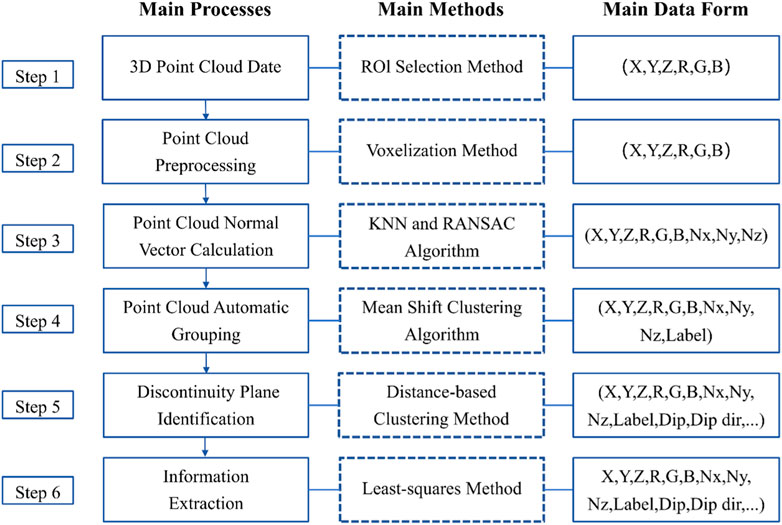
Figure 1. Discontinuous plane identification steps.

2.1.1 Point cloud voxel processing

The initial point cloud data collected through 3D laser scanning is cleaned of noise and converted into a voxel format to improve processing speed and simplify algorithm implementation. This approach dramatically decreases the amount of point cloud data, enhances computational efficiency, and preserves essential geometric characteristics by dividing the three-dimensional space into consistent voxel grids. After voxelization processing, the data maintain original accuracy and exhibit enhanced regularity, facilitating the removal of noise and outliers and improving analysis precision. Figure 2 shows the comparison effect before and after point cloud voxelization.

Figure 2

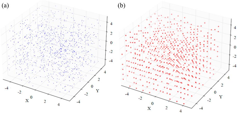
Figure 2. Point cloud voxel processing; (A) Spatial point cloud, (B) Voxelized point cloud.

2.1.2 Point cloud normal vector calculation

This research combines the K-nearest neighbor search (KNN) method with the random sample consensus (RANSAC) algorithm to improve the precision and reliability of normal vector computations for point cloud data. The process of calculating normal vectors starts by randomly choosing a point p from the point cloud to serve as the center and setting a parameter K to indicate the number of neighboring points. The KNN algorithm is then used to calculate the distances between point p and other points, with the closest K points creating the neighborhood point set N(p). This approach ensures that the chosen neighborhood points accurately reflect the spatial characteristics, which are essential for the following normal vector calculations.

The point ‘p' refers to an arbitrary point selected from the point cloud data, serving as the center for subsequent calculations. The neighborhood point set ‘N(p)' is a collection of the K nearest points around p, determined by the KNN search. Specifically, for each point p (x_p,y_p,z_p), the distance to all other points q (x_q, y_q, z_q) in the point cloud can be calculated by Equation 1:

$\text{Distance}\left(\mathrm{p},\mathrm{q}\right)=\sqrt{{\left({\mathrm{x}}_{\mathrm{q}}-{\mathrm{x}}_{\mathrm{p}}\right)}^2+{\left({\mathrm{y}}_{\mathrm{q}}-{\mathrm{y}}_{\mathrm{p}}\right)}^2+{\left({\mathrm{z}}_{\mathrm{q}}-{\mathrm{z}}_{\mathrm{p}}\right)}^2}(1)$

The K points with the smallest distances are identified as the neighborhood N(p), forming a local cluster of points that approximate the spatial characteristics surrounding p.

After obtaining the neighborhood point set, the RANSAC algorithm is applied to perform plane fitting. Specifically, three points are randomly chosen from N(p) to construct a plane model, represented by the Equation 2:

$\text{Ax}+\text{By}+\text{Cz}+\mathrm{D}=0(2)$

Here, the normal vector (A, B, C) defines the plane’s orientation. The distance d from each neighborhood point to the plane can be calculated by Equation 3:

$d=\frac{\left|A\right.x_0+B{y}_0+C{z}_0\left.+D\right|}{\sqrt{A^2+B^2+C^2}}(3)$

The coordinates of a neighborhood point are represented as (x₀, y₀, z₀). To assess the quality of the plane model, a threshold ε is used to differentiate between inliers and outliers. This process is repeated several times to improve the reliability of the normal vector estimation, keeping track of the number of inliers in each iteration. The model with the most inliers is chosen as the final plane model, and the associated normal vector (A, B, C) is determined. To maintain consistency, the outer normal vector is selected so that part of the fitting plane extends outward from the center point, ensuring that C is greater than 0.

The combination of KNN and RANSAC greatly improves the accuracy and reliability of normal vector estimation. The point set obtained from KNN offers a variety of candidate samples for RANSAC, which enhances the initial point selection process. Furthermore, KNN’s quick neighborhood search lowers the computational demands of RANSAC. Consequently, this approach enables dependable normal vector estimation in point cloud data. Figure 3 is a point cloud normal vector calculation diagram.

Figure 3

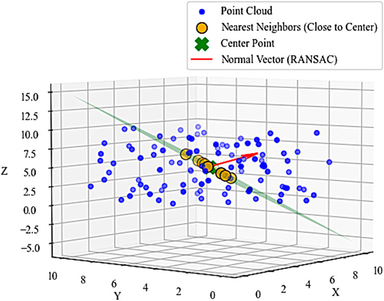
Figure 3. Normal vector calculation diagram.

2.1.3 Point cloud data clustering

The mean shift clustering algorithm initiates by selecting a random point from the point cloud as a starting point and identifying all points within a predefined distance. Figure 4 shows its working process. It computes the average coordinates of the selected points, uses this position to reselect points within the same distance, and iterates the process. By iteratively performing these steps, the algorithm navigates through the point cloud to locate the centroid of the densest point cluster. Unlike other clustering algorithms, mean shift leverages local point connectivity to converge toward cluster centroids. A key advantage of this algorithm is that it does not require a predefined number of clusters and demonstrates resilience to noise in the data.

Figure 4

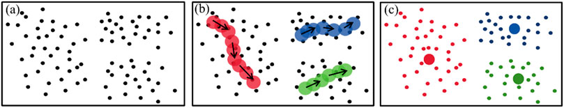
Figure 4. Mean shift clustering diagram; (A) Out-of-order point cloud, (B) Window drift, (C) Clustering out-of-order point cloud using MS (three more significant points are density centers).

The point cloud data is grouped using the mean shift algorithm, which involves the following steps:

Step 1: Define the bandwidth parameter h to determine the mean shift window size, typically ranging from 0.1 to 1 based on data characteristics.

Step 2: For each point p ∈ P (point cloud data set), identify its neighborhood point set N(p) within the bandwidth h range and calculate the mean shift vector to guide p toward a high-density region. The mean shift vector can be calculated by Equation 4:

$\text{Mean\hspace{0.17em}Shift}\left(p\right)=\frac{{\sum }_{q\in N\left(p\right)}K\left(\frac{p-q}{h}\right)\cdot q}{{\sum }_{q\in N\left(p\right)}K\left(\frac{p-q}{h}\right)}(4)$

where K is a Gaussian kernel function, and q represents a neighborhood point.

Step 3: Update the position of p using the mean shift vector and repeat Step 2 until the movement of p is less than a predefined threshold ε, the whole process can be determined by Equation 5:

$\parallel p_{new}-p_{old}\parallel <ϵ(5)$

At this stage, p is considered converged.

Step 4: According to the position of the point after convergence, the similar points are clustered into the same class. By clustering the final position of each point, the final clustering result Q = {(p₁, p₂, … )} is obtained.

2.1.4 Discontinuous surface identification and screening

Mean shift clustering produces density-based results that highlight clustering trends and enable preliminary rough classification but operate as an unsupervised method. Figure 5 shows the Euclidean distance clustering diagram. However, this approach can lead to fragmented results with excessive clustering centers. Integrating mean shift clustering results with Euclidean clustering enables merging small clusters, noise elimination, and structural simplification by adjusting cluster centers (Lab represents different point cloud sets). The clustering can be refined and validated by setting an appropriate distance threshold, allowing occurrence information extraction for each discontinuity.

Figure 5

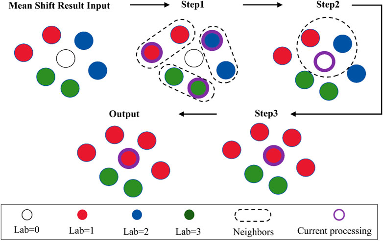
Figure 5. Euclidean distance clustering diagram.

The refinement process consists of the following steps: Step 1: Choose a specific point in the space and find its k nearest neighbors through a k nearest neighbor search. Step 2: If the distance from a point to the center point is less than a predetermined threshold d, that point is added to set B. Step 3: Select points in set B that differ from point A and repeat steps 1 and 2 until no new points are added to set B. To accurately identify primary discontinuity surfaces and remove fragmented or irregular non-primary surfaces, a screening threshold m is established. Point sets with fewer points than m are categorized as non-primary discontinuity surfaces and are excluded from information extraction and statistical analysis, while those with more than m points are deemed effective discontinuity surfaces.

2.2 Analysis of influencing factors

Sandstone samples were created as standard cylinders for direct shear and Brazilian splitting tests, measuring 50 mm in diameter and 100mm and 25 mm in height, respectively. After compression and shearing, the specimens were broken into upper and lower parts. The upper part was chosen for further analysis, and a three-dimensional topography device produced high-density point cloud data via non-contact scanning to obtain sectional details. CloudCompare software was utilized to visualize the scanned images and store the point cloud data, achieving a recorded density of 2,400/mm². The Brazilian splitting shear section of the specimen is shown in Figure 6A, and the tensile failure interface is shown in Figure 6B.

Figure 6

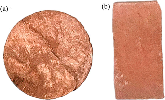
Figure 6. Three-dimensional morphology of specimen fractures after (A) shearing and (B) tension.

The point cloud data from the Brazilian splitting test were analyzed to evaluate factors influencing the recognition of discontinuous surfaces. Three parameters were manually configured: bandwidth (h), distance threshold (d), and screening threshold (m).

2.2.1 Bandwidth h

Based on Brazilian splitting test results, the mean shift clustering algorithm was employed to identify discontinuities in the point cloud data. Different bandwidth parameters (h = 0.2, 0.4, 0.6, 0.8) were evaluated to determine their effect on identifying discontinuities. The findings are illustrated in Figure 7. With h = 0.2, six sets of discontinuities were detected. The clustering outcomes were sensitive to minor discontinuities and provided detailed distributions, but there was evidence of overfitting. In contrast, with h = 0.6 and h = 0.8, only three and two discontinuous sets were identified, respectively. While the main structural planes were preserved, some finer details were lost due to overly coarse results.

Figure 7

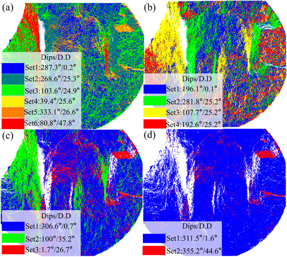
Figure 7. The influence of different bandwidths on the recognition results of discontinuities, (A) h = 0.2, (B) h = 0.4, (C) h = 0.6, (D) h = 0.8.

After thorough analysis, a bandwidth parameter of h = 0.4 produced four distinct sets, leading to more balanced and sensible clustering outcomes. This setting accurately represented the distribution patterns of significant discontinuous surfaces, prevented excessive segmentation of minor discontinuities, and successfully balanced the overall structure with local details, matching real-world conditions effectively. Therefore, h = 0.4 was chosen as the ideal bandwidth parameter.

2.2.2 Distance threshold d

The recognition results of the mean shift clustering algorithm with h = 0.4 were processed using Euclidean clustering, with the distance threshold d adjusted to 0.1, 0.2, 0.3, and 0.4. The results of discontinuous surface recognition are illustrated in Figure 8.

Figure 8

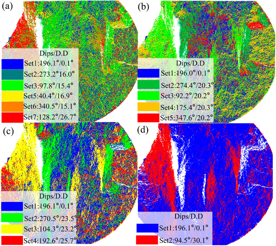
Figure 8. The influence of different distance thresholds d on the recognition results of discontinuities; (A) d = 0.1, (B) d = 0.2, (C) d = 0.3, (D) d = 0.4.

As illustrated in Figure 8, for d = 0.1 and 0.2, the distributions of dip angles and inclination values are more varied, showing notable differences among groups, which suggests a retention of more localized characteristics. In the case of d = 0.3, four distinct sets of discontinuities were found, with a reasonable merging of similar structural planes. The dip angle and inclination values obtained showed good concentration and balance. In contrast, for d = 0.4, the clustering results leaned towards global trends, resulting in the loss of some finer details. After comparing the recognition outcomes, d = 0.3 was the best parameter. At this value, the four identified discontinuity sets strike a balance between overall structure and local features, aligning with real-world conditions and accurately representing the spatial distribution of discontinuities.

2.2.3 Screening threshold m

The effect of varying the screening threshold m was observed to analyze its impact on screening results. Threshold values of m = 100, 200, 300, and 400 were evaluated.

Figure 9 shows the influence of different screening thresholds (m = 100, 200, 300, 400) on discontinuity recognition results and changes in the stereographic projection of the lower hemisphere. It can be seen from the diagram that when the screening threshold m is 100, the number of structural planes is higher, indicating that more structural planes are retained. These structural planes include small-scale noise and detail discontinuities. Secondly, the cloud image represents the density distribution of each region. The darker the color, the higher the density. At low thresholds, the distribution of high-density regions in the figure is more dispersed, indicating that these regions contain a large number of local details and discontinuities. At this time, the change of density is more complex, indicating that many small-scale structural planes are gathered together, resulting in local details and noise being preserved. As the screening threshold gradually increases (m = 400), the number of structural planes decreases, and the density distribution becomes more concentrated. This indicates that a higher screening threshold excludes minor local details that may contain noise and only retains a larger area of the main discontinuities.

Figure 9

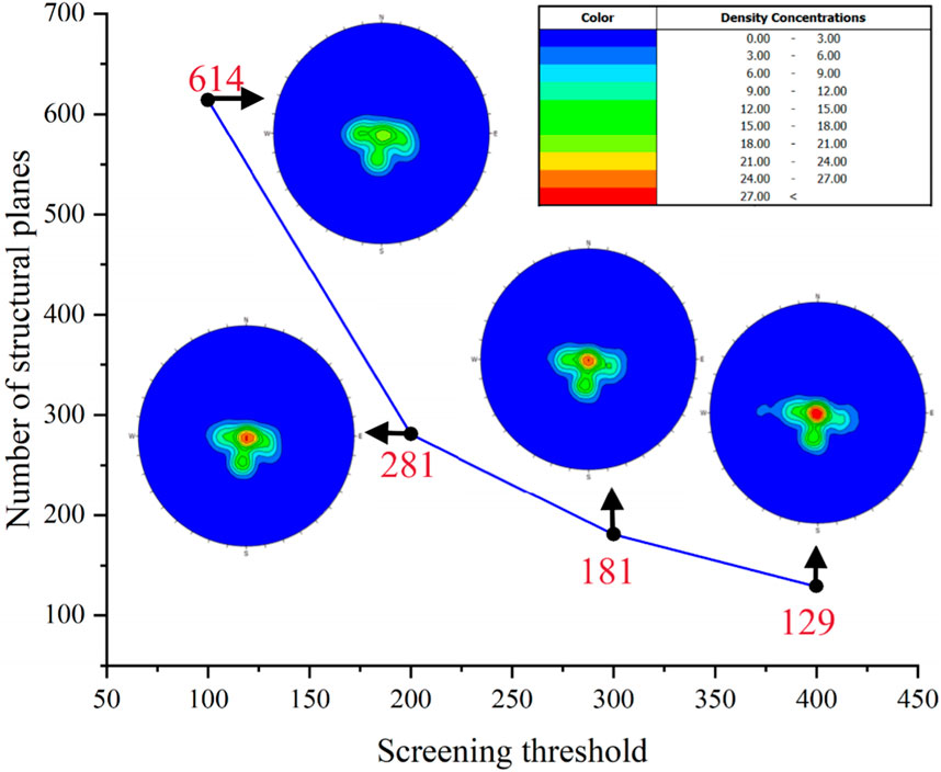
Figure 9. Statistical analysis of the influence of different screening thresholds m on the number of discontinuous surfaces.

In this discontinuity recognition process, m = 200 was selected as the final screening threshold for its balance between overall trends and local detail retention. Specifically, at m = 200, the number of discontinuities reduces to 281, significantly lower than at m = 100, effectively filtering out small-scale noise and secondary structural planes. The projection illustrates a clear and concentrated high-density discontinuity area with reduced noise interference, yielding more concise and reliable results for subsequent analysis.

2.3 Discontinuous surface information extraction

2.3.1 Extraction of dip angle tendency of discontinuous surface

After dividing the structural plane by clustering twice, the plane fitting can be carried out by the least square method, and the plane equation ax + by + c = z can be obtained, which can be expressed in matrix form as Equation 6:

$\left[\begin{array}{ccc}x& y& 1\end{array}\right]\left[\begin{array}{c}a\\ b\\ c\end{array}\right]=z(6)$

Let the coordinates of n points on the structural plane be (x₁, y₁, z₁), (x₂, y₂, z₂), (x_n, y_n, z_n), then the above equation can be expressed as Equation 7:

$\left[\begin{array}{ccc}{x}_1& y_1& 1\\ x_2& y_2& 1\\ ⋮& ⋮& ⋮\\ x_n& y_n& 1\end{array}\right]\left[\begin{array}{c}a\\ b\\ c\end{array}\right]=\left[\begin{array}{c}{z}_1\\ z_2\\ ⋮\\ z_n\end{array}\right](7)$

Let:

$A=\left[\begin{array}{c}a\\ b\\ c\end{array}\right],x=\left[\begin{array}{ccc}{x}_1& y_1& 1\\ x_2& y_2& 1\\ ⋮& ⋮& ⋮\\ ⋮& ⋮& ⋮\\ x_n& y_n& 1\end{array}\right],z=\left[\begin{array}{c}{z}_1\\ z_2\\ ⋮\\ ⋮\\ z_n\end{array}\right](8)$

Then the vector A is found by Equation 8, so that $\parallel \text{Ax}-\mathrm{z}\parallel$ obtains the minimum value, that is, the plane equation and its normal vector are obtained by fitting.

If we consider the unit normal vector of the rock mass structural plane as (a, b, c), the three-dimensional laser scanner is only able to scan the visible surface, which means c must be greater than 0. Therefore, (a, b, c) represents the unit outward normal vector of the fracture structural plane. In the geodetic coordinate system, we define the positive Y-axis as north, the positive X-axis as east, and the positive Z-axis as upward. Using the following formula, the strike α and dip angle β of rock mass structural plane in the geodetic coordinate system are determined by Equation 9:

$\left\{\begin{array}{c}\beta =\mathit{arccos}\left(c\right)\\ \text{if\hspace{0.17em}}a\ge 0,b\ge 0,\alpha =\mathit{arcsin}\left(a/\mathit{sin}\beta \right)\\ \text{if\hspace{0.17em}}a<0,b>0,\alpha =360-\mathit{arcsin}\left(-a/\mathit{sin}\beta \right)\\ \text{if\hspace{0.17em}}a<0,b<0,\alpha =180-\mathit{arcsin}\left(a/\mathit{sin}\beta \right)\\ \text{if\hspace{0.17em}}a>0,b<0,\alpha =180+\mathit{arcsin}\left(-a/\mathit{sin}\beta \right)\end{array}\right.(9)$

2.3.2 Discontinuous surface area information extraction

This paper employs a grid-filling technique to determine the area of the structural plane based on the plane fitting outcomes from the point cloud data. The fitted plane is divided into uniform grids, each with an area of one unit. A grid is deemed effective if its number of points surpasses a specified threshold; if not, it is labeled ineffective. The area of the structural plane is calculated by tallying the effective grids.

2.4 Discontinuous surface recognition results

According to the analysis presented in Section 2.2 and the point cloud data from the direct shear and Brazilian splitting tests, discontinuous surfaces were detected using parameters h = 0.4, d = 0.3, and m = 200. Figure 10 shows that four primary sets of discontinuities were found in both tests, with distinct colors effectively illustrating the spatial distribution of these surfaces. In the direct shear test, the distribution of discontinuous sets appears more random and denser, indicating a complex path of fracture propagation under shear forces characterized by fractures in multiple directions. Conversely, the Brazilian splitting test shows a distribution of discontinuous sets that is more directional, with cracks propagating along the principal stress direction. This pattern indicates a greater likelihood of penetrating fractures occurring under tensile conditions.

Figure 10

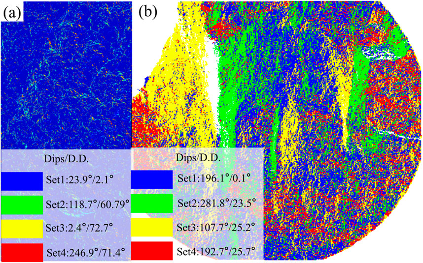
Figure 10. Sandstone section discontinuity identification results (A) Brazil splitting and (B) Direct shear test identification results.

Figure 11 illustrates the occurrence data for the sandstone section. The findings from the identification of discontinuous surfaces indicate that the occurrence data from the direct shear test is primarily found in areas with lower dip angles, with average occurrences of 196.1°∠0.1°, 281.8°∠25.3°, 107.7°∠25.2°, and 192.7°∠25.7°. This suggests that shear forces lead to a more concentrated distribution of dip angles for discontinuous surfaces, highlighting the direction and pattern of shear fractures. In contrast, the occurrence of discontinuities observed in the Brazilian splitting test spans a broader range of dip angles, with average occurrences of 23.9°∠2.1°, 118.7°∠60.79°, 2.4°∠72.7°, and 246.9°∠71.4°. This indicates that under tensile forces, the section is primarily influenced by discontinuities with steeper dip angles. The variation in occurrence distribution underscores how different loading methods affect the fracture behavior of the sandstone section.

Figure 11

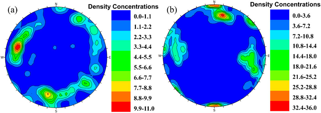
Figure 11. Sandstone section occurrence information stereo projection, (A) Brazil splitting, and (B) Direct shear test identification results.

2.5 Regular hexahedron verification

CloudCompare software was used to create point cloud data for a regular hexahedron, which has a side length of 1 cm and consists of 10,000 points on each face. The proposed algorithm was applied with a parameter k = 3, dividing the hexahedron into three groups. By setting d = 1, the six surfaces were successfully identified, with planes with the same normal vector being assigned the same color. Since the regular hexahedron has no non-primary discontinuities, screening was unnecessary.

Assuming the positive x-axis points east, the positive y-axis points north, and the z-axis points upward, the six planes of the cube were calculated to be at angles of 0°∠0°, 0°∠180°, 90°∠90°, 90°∠180°, 90°∠270°, and 90°∠360°. The area of each of the six planes is 1 m². The recognition and extraction results effectively demonstrate the proposed algorithm’s accuracy.

3 Application analysis of rock slope

The previous section used the hexahedron with known parameters to verify the algorithm’s accuracy. This section collects the point cloud data of the rock slope on-site for analysis to illustrate the algorithm’s applicability.

3.1 Rock point cloud data acquisition

Terrestrial laser scanning (TLS) mainly involves a laser rangefinder and an angle measurement system. The laser rangefinder is responsible for measuring distances, while the angle measurement system captures the angles of the laser in both horizontal and vertical planes. The scanner’s motor methodically scans the target area line-by-line and column-by-column to create a dense point cloud. This point cloud data is made up of spatial points, and after a rigid transformation, the relative positions of the points and the overall shape of the point cloud remain consistent. This research employs the MapTek I-Site 8820 for field data collection, which features a scanning field angle of 360° horizontally and 160° vertically, a measurement accuracy of ±6 mm, a maximum scanning distance of 2000 m, and an effective scanning range of 600 m (for objects with reflectivity over 10%) to 1,600 m (for objects with reflectivity over 80%). Figure 12A, B show the scanner in action in the field and the process of calculating the local coordinate system (x′, y′, z′) for each point. The high-resolution point cloud obtained is connected to geodetic coordinates (x, y, z) through the local coordinate system, with the rock point cloud data depicted in Figure 12C.

Figure 12

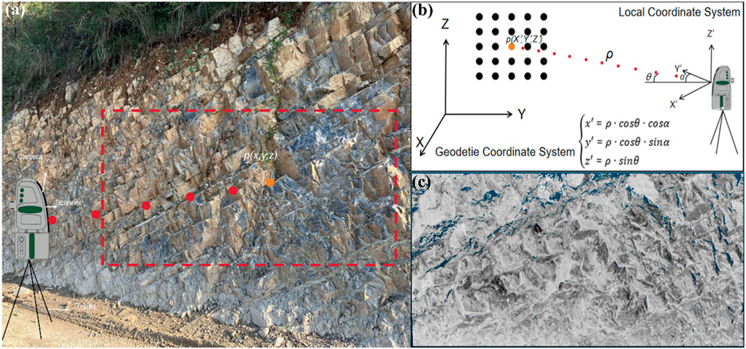
Figure 12. Data acquisition based on TLS (A) TLS work (B) Convert point cloud to geodetic coordinate system (C) Point cloud data.

3.2 Grouping results of different methods

The connection between parameter selection and the identification of rock discontinuities makes it challenging to automate the outcomes of various segmentation algorithms fully. qFacet is a widely utilized open-source algorithm for analyzing point cloud data related to rock masses, so we have chosen it as a benchmark to evaluate the effectiveness of our proposed method.

The qFacet algorithm operates as a plug-in module within Cloudcompare. It divides the original point cloud data into distinct sub-units for plane fitting and combines these plane objects into polygonal discontinuities based on a flatness threshold. By adjusting the parameters, the boundaries of the discontinuous surfaces are modified around the segmentation points, producing recognition results for the discontinuous surfaces and calculating attitude information, such as dip angle tendencies.

Our proposed method set the thresholds to h = 0.4, d = 0.3, and m = 200. For the qFacet algorithm, the minimum number of points required on each discontinuous surface is set to 200, with a minimum side length of 0.05 and a maximum distance of 0.2. The field point cloud data collected is manually segmented into two regions of interest (ROI): region I and region II. The results of the discontinuous set extraction from both our method and the qFacet method are illustrated in Figure 13.

Figure 13

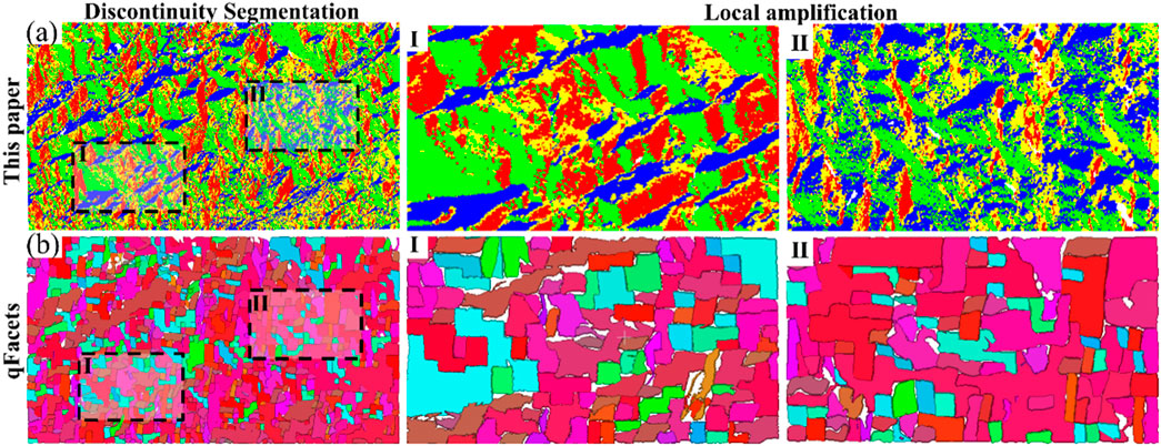
Figure 13. Discontinuous surface identification results using two methods; (A) The method proposed in this paper, (B) The qFacet method.

3.3 Discontinuity identification and measurement accuracy comparison

To assess the accuracy of the method presented in this paper, we extract information about each discontinuous set from the recognition results in the region I, as illustrated in Figure 14A. Different colors indicate various discontinuous sets, showcasing the distribution of rock discontinuities. Following the approach outlined in Section 2.3.1, we provide area statistics for the discontinuous surfaces after each screening group. In Figure 14C, the horizontal axis represents the area intervals, while the vertical axis shows the frequency percentage. The statistical analysis revealed a total of 415 discontinuous surfaces. Set 1 comprised 65 surfaces with a maximum area of 0.39 m², while Set 4 consisted of a vertical discontinuous set with 113 surfaces. Set 3 was divided into 124 discontinuous surfaces, with a dip angle similar to the original slope. The largest group, set 2, included 113 discontinuous surfaces, with a maximum area of 0.57 m².

Figure 14

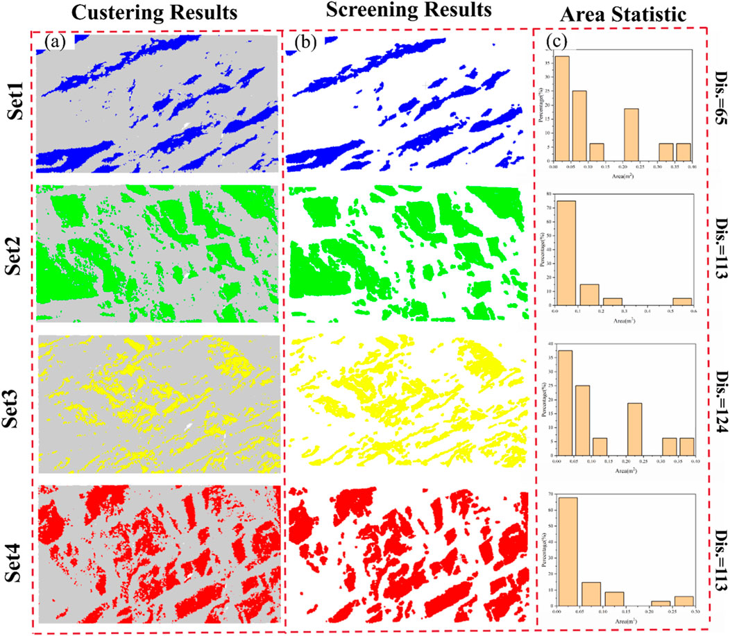
Figure 14. Region I Discontinuous set extraction results (A) each group of discontinuous set details (B) discontinuous set m = 200 screening results (C) area statistics.

Table 1 presents a comparison between the results of discontinuous surface recognition achieved by the method in Region I and those obtained through manual recognition. Initially, a representative rock layer or discontinuous surface is selected for manual dip angle measurement to avoid damaging the rock surface. A geological compass is placed flat on the rock surface to ensure proper contact and prevent tilt or misalignment. The inclination refers to the angle of the rock surface in relation to the horizontal plane, typically read on the compass dial, which ranges from 0° (horizontal) to 90° (vertical). The tendency indicates the direction of the intersection between the rock layer and the horizontal plane, measured clockwise from north, ranging from 0° to 360°. After completing the measurements, the inclination and tendency data are recorded and taken multiple times to ensure precision. The results show that the difference between the discontinuity occurrence identified by this method and the manual identification is within 1.5°.

Table 1

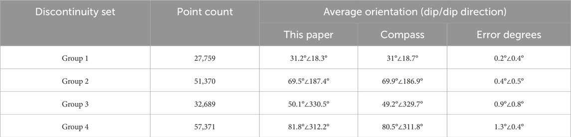
Table 1. Comparison of discontinuous surface measurement results between this method and the manual method.

Region II, which exhibits a higher degree of weathering, is chosen for comparison to assess the effectiveness of the method presented in this paper. The point cloud data from Region II displays more intricate spatial distribution and discontinuous surface features, allowing for a more thorough evaluation of the method’s performance in complex scenarios. The area distribution of the four sets of discontinuities follows a lognormal distribution. In the recognition results for the discontinuous sets in Region II, three representative discontinuous surfaces from each set are selected, totaling 12 surfaces. A comparison with the extraction results from the qFacet method is conducted, focusing on the dip angle and trend. The findings in Table 2 indicate a strong alignment between this method and qFacet in terms of dip angle and trend extraction. The maximum errors in the inclination angles for the 12 discontinuities are 1.6° and 1.3°, respectively, demonstrating the method’s high accuracy and reliability in extracting the inclination angles of the discontinuities. Additionally, this confirms the method’s robustness.

Table 2

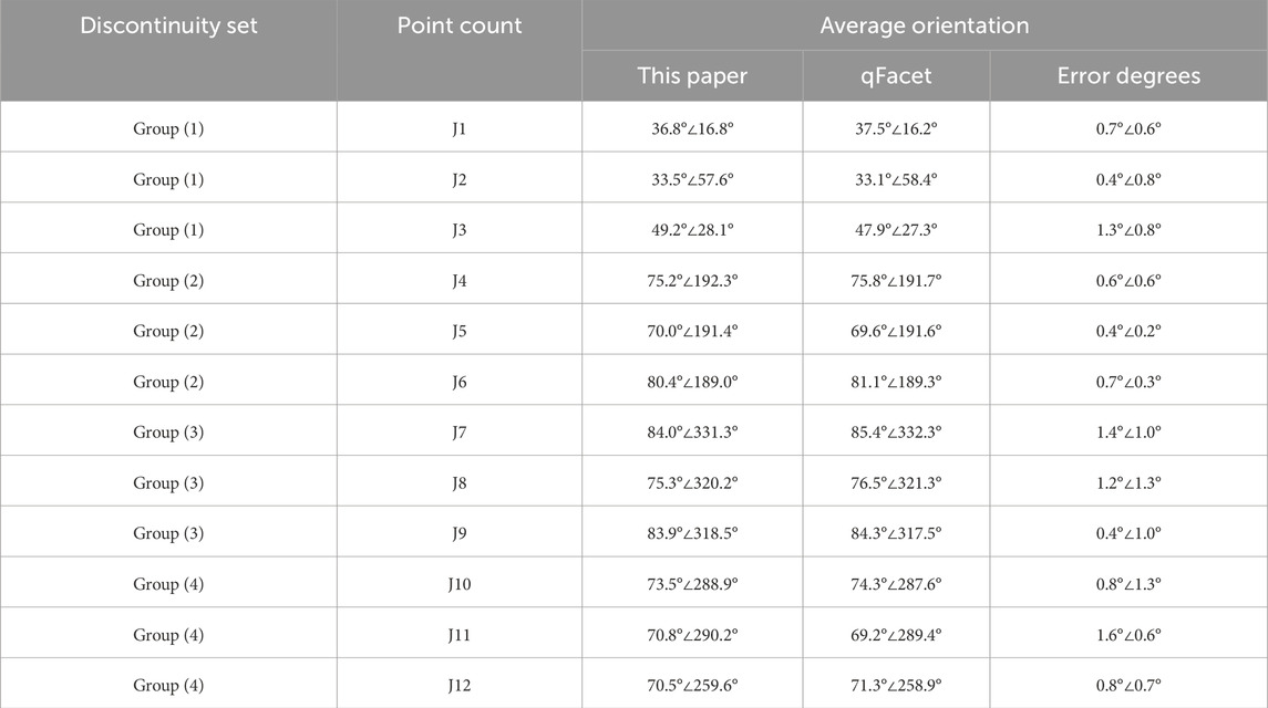
Table 2. The method in this paper is compared with the discontinuous surface measurement results of qFacet.

4 Discussion

Point cloud data is vast, and its processing requires significant computational resources and time, which is a major drawback. To address this issue, the algorithm presented in this paper aims to streamline the process and enhance calculation speed while keeping the error margin within 5%. Although down-sampling can decrease the number of points, it also results in some loss of information and accuracy. Further research is needed to minimize information loss during down-sampling.

The analysis of various influencing factors reveals that h, d, and m significantly impact the recognition outcomes of discontinuous surfaces. The algorithm can effectively detect the discontinuous surfaces within rock masses by fine-tuning these parameters. The choice of parameters is closely linked to the geometry of the object and the density of the point cloud, meaning there is no one-size-fits-all parameter. However, based on how threshold selection affects recognition results, recommendations for parameter choices under varying conditions can be made. The bandwidth h should be selected from a range of 0–1.0, starting at 0.2 and increasing incrementally, with the h value yielding the best grouping result being chosen. The distance threshold d indicates the maximum allowable distance between points and should exceed the spacing of the point cloud, with its selection depending on the density of the point cloud in different scenarios; in this study, d = 0.3 is identified as the optimal distance threshold. The screening threshold m sets the minimum number of nodes for the discontinuous surface, influencing the fragmentation of the surface and the accuracy of its identification. During actual scanning, selecting a representative small-scale area to minimize the number of point cloud data nodes is advisable. Applying the proposed algorithm to intelligently identify the discontinuity surface, swiftly obtain recognition results under various parameters, and compare these with actual measurements. This analysis will help select the most appropriate parameters, which can be applied to extensive point cloud data processing.

5 Conclusion

This study proposes a discontinuous surface recognition method based on point cloud data and verifies its applicability under various fracture modes through experimental analysis. The method demonstrates high precision, broad applicability, and robust performance in identifying and extracting rock sections’ occurrence, area, and surface morphology, as validated by hexahedron and field data analysis. The specific conclusions are summarized as follows:

(1) Combining the KNN and RANSAC algorithms improves both the speed and accuracy of normal vector calculations. The point cloud data is organized by integrating mean shift clustering with Euclidean distance clustering. The parameters for h, d, and m are established, effectively facilitating the identification and screening of discontinuities. Additionally, a method for extracting the occurrence and area of these discontinuities has been proposed.

(2) The analysis of point cloud data from the direct shear and Brazilian splitting tests indicates that different loading methods significantly influence the distribution and occurrence of discontinuities. In the direct shear test, the distribution of discontinuities is relatively concentrated, with a small dip angle, demonstrating a clear directional pattern that reflects the regularity of shear fractures. Conversely, in the Brazilian splitting test, the distribution of discontinuities is more complex and random, with discontinuities exhibiting larger dip angles being predominant. This reveals the multi-directional fracture characteristics that occur under tensile forces.

(3) The discontinuity identification method proposed in this paper was validated using both regular hexahedron data and field data, demonstrating its high precision and broad applicability. In the hexahedron validation, the algorithm successfully identified six faces and extracted occurrence and area information that aligns with theoretical expectations. In the field data validation, comparison results with the qFacet algorithm indicate that the proposed method exhibits high consistency in dip angle and trend extraction, with a minimal error margin (≤1.5°). Notably, the proposed method in complex rock formations effectively identifies small-scale discontinuities and accurately calculates their areas, confirming its reliability and robustness in practical applications.

Data availability statement

The original contributions presented in the study are included in the article/supplementary material, further inquiries can be directed to the corresponding author.

Author contributions

LZ: Investigation, Software, Writing–original draft. SL: Data curation, Formal Analysis, Writing–original draft. TL: Data curation, Investigation, Writing–original draft. XS: Data curation, Formal Analysis, Methodology, Writing–original draft. FR: Conceptualization, Methodology, Supervision, Writing–review and editing.

Funding

The author(s) declare that financial support was received for the research, authorship, and/or publication of this article. This research was supported by the Zhongjiao Hehai Engineering Co., Ltd.

Conflict of interest

Authors LZ, SL, and XS were employed by Zhongjiao Hehai Engineering Co., Ltd.

The remaining authors declare that the research was conducted in the absence of any commercial or financial relationships that could be construed as a potential conflict of interest.

The authors declare that this study received funding from Zhongjiao Hehai Engineering Co., Ltd. The funder had the following involvement in the study: the funder offers assistance with data collection.

Generative AI statement

The author(s) declare that no Generative AI was used in the creation of this manuscript.

Publisher’s note

All claims expressed in this article are solely those of the authors and do not necessarily represent those of their affiliated organizations, or those of the publisher, the editors and the reviewers. Any product that may be evaluated in this article, or claim that may be made by its manufacturer, is not guaranteed or endorsed by the publisher.

References

Bendezu, D. L. C. M. A. (2021). Evaluation of LIDAR systems for rock mass discontinuity identification in underground stone mines from 3D point cloud data. West Virginia Univ. doi:10.33915/etd.10243

CrossRef Full Text | Google Scholar

Chen, N., Xiao, A., Li, L. H., and Xiao, H. L. (2024). Semi-automatic identification of tunnel discontinuity based on 3D laser scanning. Geotech. Geol. Eng. 42 (4), 2577–2599. doi:10.1007/s10706-023-02692-2

CrossRef Full Text | Google Scholar

Ge, Y., Cao, B., and Tang, H. (2022). Rock discontinuities identification from 3D point clouds using artificial neural network. Rock Mech. Rock Eng. 55 (3), 1705–1720. doi:10.1007/s00603-021-02748-w

CrossRef Full Text | Google Scholar

Gu, Z., Xiong, X., Yang, C., and Cao, M. (2024). A method for identification rock mass discontinuities in underground drift with pre-separation of linear and planar point cloud features. Ain. Shams. Eng. J. 15, 103110. doi:10.1016/j.asej.2024.103110

CrossRef Full Text | Google Scholar

Hudson, R., Faraj, F., and Fotopoulos, G. (2020). Review of close-range three-dimensional laser scanning of geological hand samples. Earth-Sci. Rev. 210, 103321. doi:10.1016/j.earscirev.2020.103321

CrossRef Full Text | Google Scholar

Jiang, S., Jiang, W., and Wang, L. (2021). Unmanned aerial vehicle-based photogrammetric 3D mapping: a survey of techniques, applications, and challenges. IEEE Geosc. Rem. Sen. M. 10 (2), 135–171. doi:10.1109/MGRS.2021.3122248

CrossRef Full Text | Google Scholar

Kong, D. H., Saroglou, C., Wu, F. Q., Sha, P., and Li, B. (2021). Development and application of UAV-SfM photogrammetry for quantitative characterization of rock mass discontinuities. Int. J. Rock. Mech. Min. 141, 104729. doi:10.1016/j.ijrmms.2021.104729

CrossRef Full Text | Google Scholar

Lin, Q. B., Cao, P., Wen, G. P., Meng, J. J., Cao, R. H., and Zhao, Z. Y. (2021). Crack coalescence in rock-like specimens with two dissimilar layers and pre-existing double parallel joints under uniaxial compression. Int. J. Rock. Mech. Min. 139, 104621. doi:10.1016/j.ijrmms.2021.104621

CrossRef Full Text | Google Scholar

Liu, C., Jiang, Q., Xin, J., Wu, S., Liu, J., and Gong, F. Q. (2022). Shearing damage evolution of natural rock joints with different wall strengths. Rock Mech. Rock Eng. 55 (3), 1599–1617. doi:10.1007/s00603-021-02739-x

CrossRef Full Text | Google Scholar

Liu, G., Liu, J., Luo, S., Bo, W., Kang, J., and Miao, J. (2023). Development of a composite implicit time integration scheme for three-dimensional discontinuous deformation analysis. Mathematics-Basel 11 (18), 3881. doi:10.3390/math11183881

CrossRef Full Text | Google Scholar

Liu, G. Y., Zhong, Z. R., Ma, K., Bo, W., Zhao, P. H., Li, Y. X., et al. (2024). Field experimental verifications of 3D DDA and its applications to kinematic evolutions of rockfalls. Int. J. Rock. Mech. Min. 175, 105687. doi:10.1016/j.ijrmms.2024.105687

CrossRef Full Text | Google Scholar

Liu, Q. B., Cao, P., Meng, J. J., Cao, R. H., and Zhao, Z. Y. (2020). Strength and failure characteristics of jointed rock mass with double circular holes under uniaxial compression: insights from discrete element method modelling. Theor. Appl. Fract. Mec. 109, 102692. doi:10.1016/j.tafmec.2020.102692

CrossRef Full Text | Google Scholar

Ma, L., Zuo, C., Qiu, H., Ma, H., Yang, M., Zhou, C., et al. (2024). A multilevel classification strategy for the identification of discontinuities from 3D point clouds of complicated rock surfaces. Rock Mech. Rock Eng. 57, 10611–10630. doi:10.1007/s00603-024-04109-9

CrossRef Full Text | Google Scholar

Rao, K. S. (2020). Characterization, modelling and engineering of rocks and rockmasses. Indian Geotech. J. 50 (1), 1–95. doi:10.1007/s40098-020-00414-6

CrossRef Full Text | Google Scholar

Sun, P. P., Yang, X. X., Sun, D. K., Qiao, W. G., and Wu, Y. (2020). Geometric and mechanical properties of a shear-formed fracture occurring in a rock bridge between discontinuous joints. B. Eng. Geol. Environ. 79, 1365–1380. doi:10.1007/s10064-019-01669-x

CrossRef Full Text | Google Scholar

Tang, M., Yang, S., Huang, G., Xie, X., Guo, J., and Zhai, J. (2022). Automatic extraction of rock discontinuities from the point cloud using dynamic DBSCAN algorithm. Adv. Civ. Eng. 2022 (1), 7754179. doi:10.1155/2022/7754179

CrossRef Full Text | Google Scholar

Tang, N., Wang, L., Jiang, H., Huang, X., Tan, G., and Zhou, X. (2023). A new clustering method of rock discontinuity sets based on modified K-means algorithm. B. Eng. Geol. Environ. 415, 415. doi:10.1007/s10064-023-03406-x

CrossRef Full Text | Google Scholar

Temur, M. A., Kocaman, S., and Nefeslioglu, H. A. (2024). On the use of semi-georeferenced photogrammetric dense point clouds in the investigation of rock mass discontinuity properties. B. Eng. Geol. Environ. 83 (11), 451–523. doi:10.1007/s10064-024-03947-9

CrossRef Full Text | Google Scholar

Walicka, A., and Pfeifer, N. (2022). Automatic segmentation of individual grains from a terrestrial laser scanning point cloud of a mountain river bed. IEEE J-Stars 15, 1389–1410. doi:10.1109/JSTARS.2022.3141892

CrossRef Full Text | Google Scholar

Wang, M., Zhou, J. W., Chen, J. L., Jiang, N., Zhang, P. W., and Li, H. B. (2023). Automatic identification of rock discontinuity and stability analysis of tunnel rock blocks using terrestrial laser scanning. J. Rock Mech. Geotech. 15 (7), 1810–1825. doi:10.1016/j.jrmge.2022.12.015

CrossRef Full Text | Google Scholar

Wang, S., Yin, J., Pi, Z., Cao, W., Cai, X., and Zhou, Z. (2024). Automatic detection and characterization of discontinuity traces and rock fragment size distribution using a digital image processing method. Measurement 228, 114343. doi:10.1016/j.measurement.2024.114343

CrossRef Full Text | Google Scholar

Wu, F. Q., Wu, J., Bao, H., Bai, Z. X., Qiao, L., Zhang, F., et al. (2023). Rapid intelligent evaluation method and technology for determining engineering rock mass quality. Rock. Mech. Bull. 2 (2), 100038. doi:10.1016/j.rockmb.2023.100038

CrossRef Full Text | Google Scholar

Xu, Z. H., Guo, G., Sun, Q. C., Wang, Q., Zhang, G. D., and Ye, R. Q. (2023). Structural plane recognition from three-dimensional laser scanning points using an improved region-growing algorithm based on the robust randomized Hough transform. J. Mt. Sci-Engl. 20 (11), 3376–3391. doi:10.1007/s11629-023-7914-z

CrossRef Full Text | Google Scholar

Xue, J., Xiong, S., Liu, Y., Men, C., and Tian, Z. (2023). A bottom-up method for roof plane extraction from airborne LiDAR point clouds. Meas. Sci. Technol. 35 (2), 025209. doi:10.1088/1361-6501/ad0f69

CrossRef Full Text | Google Scholar

Yang, X. X., and Qiao, W. G. (2018). Numerical investigation of the shear behavior of granite materials containing discontinuous joints by utilizing the flat-joint model. Comput. Geotech. 104, 69–80. doi:10.1016/j.compgeo.2018.08.014

CrossRef Full Text | Google Scholar

Yi, X., Feng, W., Wu, W., Zhou, Y., and Dong, S. (2023). An effective approach for determining rock discontinuity sets using a modified whale optimization algorithm. Rock Mech. Rock Eng. 56 (8), 6143–6155. doi:10.1007/s00603-023-03364-6

CrossRef Full Text | Google Scholar

Yong, R., Wang, H., Ye, J., Du, S., and Luo, Z. (2024). Neutrosophic genetic algorithm and its application in clustering analysis of rock discontinuity sets. Expert. Syst. Appl. 245, 122973. doi:10.1016/j.eswa.2023.122973

CrossRef Full Text | Google Scholar

Yu, D., Xiao, J., and Wang, Y. (2022). Efficient lightweight surface reconstruction method from rock-mass point clouds. Remote Sens-Basel 14 (5), 1200. doi:10.3390/rs14051200

CrossRef Full Text | Google Scholar

Zaczek Peplinska, J., and Kowalska, M. E. (2022). Application of non-contact geodetic measurement techniques in dam monitoring. Arch. Civ. Eng. 63 (3). doi:10.24425/ace.2022.141873

CrossRef Full Text | Google Scholar

Zhang, H. J., Wu, S. C., and Han, L. Q. (2022). Dominant partitioning method of rock mass discontinuity based on DBSCAN selective clustering ensemble. Rock Soil. Mech. 43 (6), 6. doi:10.16285/j.rsm.2021.6582

CrossRef Full Text | Google Scholar

Zhu, J., Xia, Y., Wang, B., Yang, Z., and Yang, K. (2024). Research on the identification of rock mass structural planes and extraction of dominant orientations based on 3D point cloud. Appl. Sci. 14 (21), 9985. doi:10.3390/app14219985

CrossRef Full Text | Google Scholar