Study on lithology identification using a multi-objective optimization strategy to improve integrated learning models: a case study of the Permian Lucaogou Formation in the Jimusaer Depression

Lithology identification is a critical task in logging interpretation and reservoir evaluation, with significant implications for recognizing oil and gas reservoirs. The challenge in shale reservoirs lies in the similar logging response characteristics of different lithologies and the imbalanced data scale, leading to fuzzy lithology classification boundaries and increased difficulty in identification. This study focuses on the shale reservoir of the Permian Lucaogou Formation in the Jimusaer Depression for lithology identification. Initially, a comprehensive sampling model—Smote-Tomek (ST) is used to introduce new feature information into the dataset while removing redundant features, effectively addressing the issue of data imbalance. Then, by combining the multi-objective optimization strategy Artificial Rabbit Optimization (ARO) with the Light Gradient Boosting Machine (LightGBM) model, a new intelligent lithology identification model (ST-ARO-LightGBM) is proposed, aimed at solving the problem of non-optimal hyperparameter settings in the model. Finally, the proposed new intelligent lithology identification model is compared and analyzed with six models: K-Nearest Neighbors (KNN), Decision Tree (DT), Gradient Boosting Decision Tree (GBDT), Random Forest (RF), Extreme Gradient Boosting (XGBoost), and LightGBM, all after comprehensive sampling. The experimental results show that the ST-ARO-LightGBM model outperforms other classification models in terms of classification evaluation metrics for different lithologies, with an overall classification accuracy improvement of 9.13%. The method proposed in this paper can solve the problem of non-equilibrium in rock samples, and can further improve the classification performance of traditional machine learning, and provide a method reference for the lithology classification of shale reservoirs.

1 Introduction

Lithology identification is a critical task in the field of petroleum exploration and development, influencing reservoir evaluation and geological modeling processes. Logs data, characterized by high vertical resolution and continuity, is widely used for lithology identification (Baisakhi and Rima, 2018). Currently, tight and shale oil and gas have become significant alternative resources (Feng et al., 2020; Feng et al., 2021; Feng et al., 2023; Zou et al., 2015; Passey et al., 2010). However, due to the similar logging response characteristics of different lithologies within shale reservoirs and the ambiguity and subjectivity indicated by logs parameters, traditional lithology identification methods fail to effectively classify lithologies. Additionally, the limitations of coring data result in an imbalanced lithology dataset, further leading to inaccurate lithology prediction results. Machine learning methods can effectively alleviate these issues (Al-Anazi and Gates, 2010; Saporetti et al., 2019; Bestagini et al., 2017; Bressan et al., 2020a; Imamverdiyev and Lyudmila, 2019).

Machine learning, with its strong nonlinear mapping capabilities across multiple scales and dimensions, has been widely applied to the fine identification of lithologies (Chioma et al., 2018). Prabowo UN (Prabowo et al., 2023) used the KNN clustering algorithm to accurately classify different lithofacies types in thefield Z, Indonesia. And the influence of hyperparameter K in KNN model on lithology identification results is analyzed and compared. Li, Bressan, and others (Li et al., 2023; Bressan et al., 2020b) applied support vector machine models to lithology identification. Mou Dan (Mou et al., 2021) compared the accuracy and applicability of K-Nearest Neighbors, support vector machines, and adaptive boosting algorithms in identifying volcanic rock lithologies. As exploration efforts continue to increase, the lithology in actual reservoirs becomes more complex. The fitting effect of a single model is insufficient to accurately classify the lithology types of complex reservoirs. The emergence of integrated models, which combine the classification results of multiple single models, further improves the accuracy of lithology prediction. Thongsamea et al. (2021) and Chen et al. (2024) used conventional logging curves as inputs for the XGBoost model, accurately identifying the lithologies of volcanic reservoirs. Huang et al. (2023) and Wang et al. (2020) applied the Boosting algorithm integrated with the random forest model, effectively enhancing the accuracy of lithology identification. However, the accuracy of machine learning models in predicting lithology depends on the scale of the sample set (Han et al., 2024). Machine learning is insensitive to the feature parameters of minority class samples, and different combinations of hyperparameters can affect the model’s lithology identification accuracy (Saporetti et al., 2021).

To address the above issues, this paper proposes a multi-objective optimization strategy to modify an integrated learning model (ST-ARO-LightGBM) for imbalanced sample datasets. This model incorporates ST comprehensive sampling technology to effectively solve the problem of sample imbalance. The ARO technology adaptively adjusts the model’s hyperparameter combinations to find the optimal hyperparameter set, achieving efficient and accurate lithology identification of the shale reservoir in the Permian Lucaogou Formation of the Jimusaer Depression. By integrating advanced machine learning techniques and integrated sampling methods, our study demonstrates a general approach to enhanced lithology prediction that not only addresses the challenges of data imbalance and complex lithology identification in shale reservoirs, but also provides a robust solution that can be adapted to other regions with similar geological conditions.

2 Methods and theory

2.1 Artificial Rabbit Optimization

ARO model is a novel intelligent multi-objective optimization strategy inspired by the group behaviors observed in the survival and evolution of rabbit populations (Wang et al., 2022). During their survival, rabbits primarily engage in two strategies: detouring foraging (exploration) and random digging (hiding). The transition between these strategies is mainly influenced by the rabbit’s energy factor (Formula 1). When the energy factor is high, rabbits have more stamina and are more likely to adopt exploration strategies. Conversely, when the energy factor is low, they are more inclined to adopt hiding strategies to avoid predators.

$A\left(t\right)=4\left(1-\frac{t}{T}\right)\ln \frac{1}{r}(1)$

In this context, A(t) represents the energy factor, which is a function that oscillates and gradually decreases over time t. T represents the total number of iterations of the algorithm, and r is a random number between 0 and 1.

The ARO algorithm simulates the survival and evolution process of a rabbit population to seek the optimal solution in a multi-dimensional space. Assume there is a rabbit population of N rabbits in a D-dimensional space, where the position of the ith rabbit can be represented as: $R_i=\left[R_{i1},R_{i2},R_{i3},···,R_{iD}\right]$. During the iteration process of the population, the positions of the rabbits will continuously change. The mathematical model of the exploration strategy can be represented by Formula 2, and the mathematical model of the hiding strategy can be represented by Formula 3.

$\begin{array}{ll}\hfill v_i\left(t+1\right)& =x_j\left(t\right)+\left(e-e^{{\left(\frac{t-1}{T}\right)}^2}\right)\cdot \sin \left(2\pi r_2\right)\cdot c\cdot \left(x_i\left(t\right)-x_j\left(t\right)\right)\hfill \\ \hfill & +round\left(0.5\cdot \left(0.5+r_1\right)\right)\cdot n_1\hfill \end{array}(2)$

$\begin{array}{ll}\hfill v_i\left(t+1\right)& =x_i\left(t\right)+\left(e-e^{{\left(\frac{t-1}{T}\right)}^2}\right)\cdot \sin \left(2\pi r_2\right)\cdot c\cdot \hfill \\ \hfill & \left(r_3\cdot x_i\left(t\right)+\frac{T-t+1}{T}\cdot r_4\cdot g_r\cdot x_i\left(t\right)-x_i\left(t\right)\right)\hfill \end{array}(3)$

where $v_i\left(t+1\right)$ represents the position of the ith rabbit at time t+1, and $x_j\left(t\right)$ represents the position of the jth rabbit at time t; c and g_r represent sequences in the D-dimensional space where the mth position is 1 and all other positions are 0. n₁ follows a standard normal distribution, and r₁,r₂,r₃,r₄ are random numbers between 0 and 1.

2.2 Light Gradient Boosting Machine

LightGBM is a high-performance ensemble learning algorithm based on gradient boosting trees (Ke et al., 2017). Its core idea is to iteratively train multiple weak classifiers, where each iteration generates a new decision tree to correct the prediction errors of all previous trees, thereby gradually improving the overall predictive performance of the model. The objective function of LightGBM is as follows (Formula 4):

$Ob{j}^{\left(t\right)}={\displaystyle \sum _{i=1}^n}L\left(y_i,f_{t-1}\left(x_j\right)\right)+{\displaystyle \sum _{k=1}^T}\mathrm{\Omega }\left(f_k\right)(4)$

where $Ob{j}^{\left(t\right)}$ represents the loss function at the tth iteration, ${\displaystyle {\sum }_{i=1}^n}L\left(y_i,f_{t-1}\left(x_j\right)\right)$ represents the prediction error up to the (t-1)-th iteration, and ${\displaystyle {\sum }_{k=1}^T}\mathrm{\Omega }\left(f_k\right)$ represents the regularization term.

To improve training speed, LightGBM also employs the histogram-based optimization algorithm and the leaf-wise growth strategy. The histogram-based optimization algorithm reduces computational complexity by grouping continuous feature values into discrete bins, thereby decreasing the amount of computation required during the splitting of decision trees and more effectively determining the optimal split points. The leaf-wise growth strategy selects the leaf node with the maximum gain for splitting at each iteration. Compared to the traditional level-wise growth strategy, leaf-wise can quickly find good split nodes, effectively reducing the depth of the tree and speeding up model training. Additionally, the leaf-wise strategy can handle feature imbalance more flexibly, giving the model better generalization ability.

2.3 Smote-Tomek

During exploration, there is a significant imbalance in the number of lithological types in rock thin sections. Such severe sample imbalance can cause machine learning models to overly focus on the majority class samples and ignore the characteristics of the minority class samples during the learning process (Deng et al., 2023). To address this issue, sampling algorithms are needed to balance the number of samples of different lithologies, thereby enhancing the machine learning model’s ability to analyze minority class samples. ST is a combined sampling algorithm that integrates Smote oversampling with Tomek link undersampling techniques (Pereira et al., 2020; Devi and Purkayastha, 2017). It has shown good effectiveness in addressing the problem of sample imbalance in datasets. Compared to single sampling methods, Smote-Tomek compensates for the limitations of the Smote oversampling method, which tends to focus only on the minority class samples, leading to further overlap of different types of samples and low-quality data synthesis. The specific implementation steps are as follows:

(1) For the minority class samples, calculate the distance between the minority class samples and other class samples.

(2) Based on the distance between samples, generate a new sample through linear interpolation, so that the new sample lies on the line connecting two samples

(3) In the newly generated dataset, recalculate the distances between different samples to find the nearest neighbor samples of different classes that form Tomek links, where the two samples in a Tomek link pair belong to different classes.

(4) Remove the majority class samples in the Tomek link pairs to reduce the overlap at the decision boundary of the dataset, decrease the number of majority class samples, and generate a high-quality dataset.

2.4 ST-ARO-LightGBM model

The training effectiveness of a machine learning model primarily depends on the quality of the dataset and the configuration of model parameters (Probst et al., 2019). This paper first uses the ST model to perform combined sampling on the lithological dataset in the study area, generating a new dataset. Then, the ARO multi-objective optimization strategy is used to adjust the hyperparameters of the LightGBM model, enhancing its lithological identification capability. The steps to establish the ST-ARO-LightGBM model are as follows, with the flowchart shown in Figure 1.

1. Use the ST method on the collected imbalanced lithological dataset to generate a new dataset, making the number of different lithological samples relatively balanced.

2. Based on the number m of hyperparameters to be optimized in the LightGBM model and the range of these hyperparameters, initialize the positions of N artificial rabbit individuals in the ARO population $X_i=\left[x_{i,1},x_{i,2},x_{i,3},···,x_{i,m}\right],i=1,2,···,N$, and initialize the number of algorithm iterations T.

3. Split the combined sampled data into training and testing sets. Use the values of each artificial rabbit individual X_i as the input hyperparameters for the LightGBM model, establish the LightGBM lithology prediction model, and calculate the current model’s fitness value F_best based on the testing set. The position X_best of the artificial rabbit individual corresponding to the highest fitness value is taken as the optimal hyperparameter combination for the LightGBM model.

4. For each artificial rabbit individual X_i, calculate the energy factor A. When A > 1, the artificial rabbit adopts the exploration strategy shown in Formula 2. Similarly, when A ≤ 1, the artificial rabbit adopts the hiding strategy shown in Formula 3. This process updates the positions of the artificial rabbit population.

5. For each individual in the updated rabbit population, recalculate the fitness value of the corresponding LightGBM model. If the new highest fitness value F_new is greater than F_best, update the highest fitness value F_best and the optimal hyperparameter combination X_best; otherwise, take no action.

6. Repeat steps (3) to (5) until the maximum number of iterations of the algorithm is reached. Use the optimal hyperparameter combination X_best as the input for the LightGBM model to obtain the optimal ST-ARO-LightGBM lithology identification model.

Figure 1

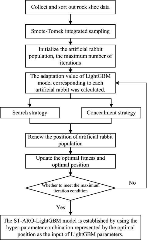
Figure 1. Flowchart of ST-ARO-LightGBM model establishment.

2.5 Model evaluation metrics

In classification tasks, the confusion matrix is commonly used to reflect the relationship between true classes and predicted classes (Sun Y. et al., 2020). For example, in binary classification tasks as shown in Table 1, the number of samples where the true class is predicted as the true class is defined as True Positive (TP). Similarly, False Negative (FN), False Positive (FP), and True Negative (TN) are defined accordingly. Based on this, four model evaluation metrics can be defined, as shown in Formula 5: Accuracy, Recall, Precision, and F1-score. Accuracy reflects the overall performance of the model, while F1-score is the harmonic mean of Recall and Precision. Higher values of these evaluation metrics indicate better classification performance of the model.

$\left\{\begin{array}{l}\text{Accuracy}=\frac{\text{TP}+\text{TN}}{\text{TP}+\text{FN}+\text{FP}+\text{TN}}\\ \text{Precision}=\frac{\text{TP}}{\text{TP}+\text{FP}}\\ \text{Recall}=\frac{\text{TP}}{\text{TP}+\text{FN}}\\ \mathrm{F}1-\text{score}=\frac{2\times \text{Precision}\times \text{Recall}}{\text{Precision}+\text{Recall}}\end{array}\right.(5)$

Table 1

Table 1. Confusion matrix for binary classification tasks.

3 Experimental dataset

3.1 Lithology types

The data of rock slices used in this paper are from Jimusaer Depression, as shown in Figure 2. The Jimusaer Depression is located in the eastern part of the Junggar Basin and overall presents a west-low east-high, west-faulted east-overlapping graben feature Lucaogou Formation in Jimusaer Depression is rich in tight oil and shale oil resources, and its shale formations are developed in two oil-bearing systems, the upper and the lower, which are characterized by the integration of source and reservoir, thin layer superposition, large thickness, whole oil-bearing and continuous distribution. Influenced by multi-source mixing and frequent changes in water bodies, the lithology of the Permian Lucaogou Formation in the study area exhibits complex and diverse characteristics (Zha, 2022; Xiong et al., 2023). As shown in Figure 3. Based on thin section and core sample data, the lithology of the Permian Lucaogou Formation is divided into four categories according to grain size and mineral composition: mudstone, cloud-bearing sandstone, siltstone, and detrital-bearing dolomite. These categories are the subjects of this study, with sample proportions of 39.49%, 38.03%, 16.00%, and 6.49%, respectively.

Figure 2

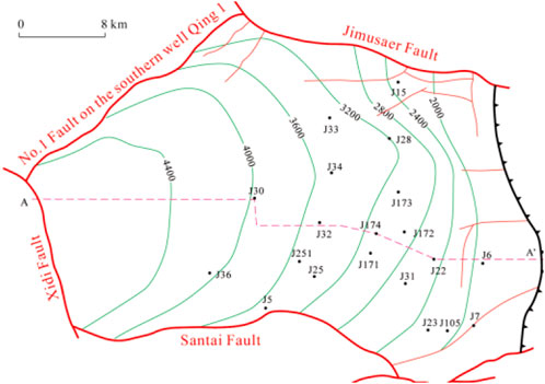
Figure 2. Geological structure map of the Jimusaer Depression.

Figure 3

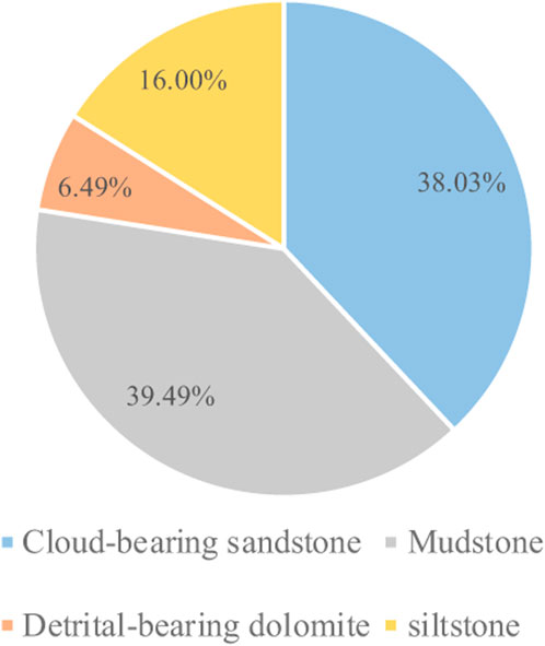
Figure 3. Pie chart of core lithology in the Permian Lucaogou Formation.

The ratio of the majority class, mudstone, to the minority class, detrital-bearing dolomite, is close to 7:1, indicating a serious imbalance in the dataset. This imbalance can cause the model to overlook the feature extraction of the detrital-bearing dolomite class during training, thereby affecting the model’s performance. This issue will be addressed in Section 4.1.

3.2 Lithological logging response characteristics

The logging response characteristics of different rock types exhibit certain differences. Conventional logging curves are a comprehensive response to the mineral composition of rocks, the nature of pore fluids, and physical properties, while nuclear magnetic resonance (NMR) logging data can reflect physical factors such as the specific surface area and shape of rock pores (Singh and Maheswar, 2022; Mitchell, 2020). Therefore, combining conventional logging curves with NMR logging data after thin section correlation, eight curves were selected to establish the lithological dataset: Acoustic travel time (AC), Compensated Neutron Log (CNL), Density log (DEN), Natural Gamma Ray (GR), Deep Resistivity (RT), Shallow Resistivity (RXO), T2 geometric mean (T_2LM), and Total Porosity from NMR (POR).

The study of the distribution of logging response parameters for different lithologies is fundamental for lithological identification. Therefore, it is necessary to statistically analyze the logging parameters of different lithologies within the study area, as shown in Table 2.

Table 2

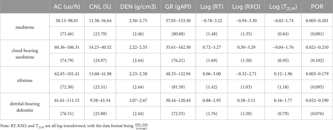
Table 2. Statistics on the range of logging response parameters for different lithologies.

As shown in Figure 4, the box diagram can better describe the distribution range of logging parameters for each lithology. The lower boundary of the box represents the first quartile, i.e. 25% of the data is less than or equal to this value, the upper boundary represents the third quartile, and the black line in the middle of the box represents the median. The box plots of logging parameters for different lithologies indicate that mudstone exhibits characteristics of medium-high DEN, medium-high GR, medium-low RT, and medium-low POR. Cloud-bearing sandstone shows characteristics of medium AC, medium-low GR, medium-high RXO, and medium-high POR. Siltstone displays low AC, medium-high GR, medium-low RXO, and medium-high T_2LM. Detrital-bearing dolomite exhibits medium-low GR, medium-high RT, medium-low T_2LM, and medium-low POR. Different logging parameters reflect different physical information of the rocks (Sebtosheikh et al., 2015). However, there is no distinct separation between different lithologies based on single logging parameters alone. Therefore, it is necessary to integrate multiple logging parameters and use multidimensional, multi-scale machine learning methods for efficient data analysis to classify lithologies.

Figure 4

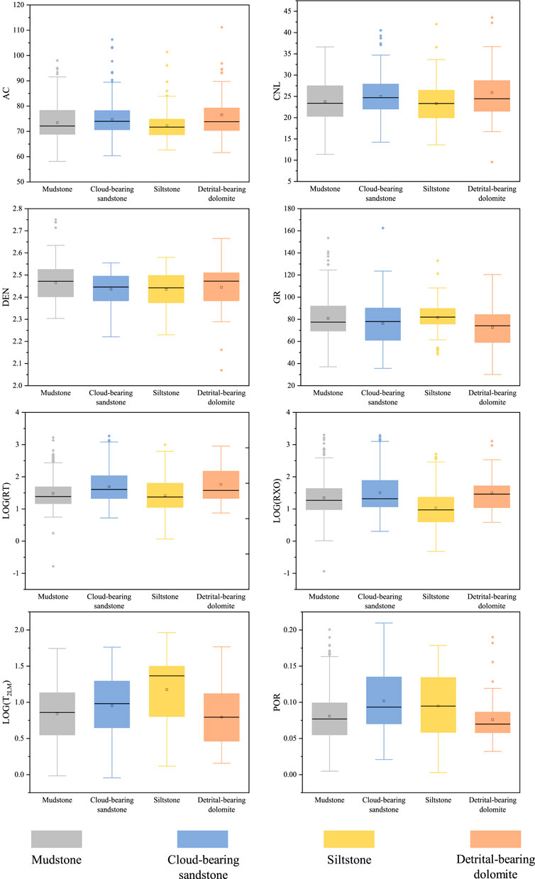
Figure 4. Box plots of logging parameters for different lithologies.

4 Experiments

4.1 Comprehensive sampling effect

In this study, a total of 895 core thin section samples were collected, including 353 mudstone samples, 341 cloud-bearing sandstone samples, 143 siltstone samples, and 58 detrital-bearing dolomite samples. The imbalance in sample numbers can cause the classifier to fail to adequately extract features from minority class samples, thus affecting its ability to classify minority class samples and reducing the model’s generalizability and accuracy. To address this issue, the ST algorithm was employed for comprehensive sampling of the dataset. The sampling results are shown in Figure 5. The number of samples for siltstone and detrital-bearing dolomite increased, introducing new feature information to the dataset. The number of samples for mudstone and cloud-bearing sandstone slightly decreased, removing some redundant features of the majority classes. The overall dataset has now reached a balanced state after sampling.

Figure 5

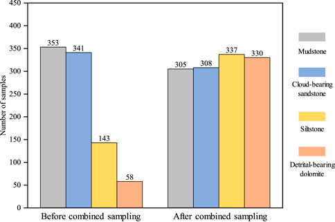
Figure 5. Comparison of the number of samples before and after combined sampling.

To verify the impact of ST combined sampling on the performance of the LightGBM model, this study splits the datasets before and after ST combined sampling into training and testing sets in a 7:3 ratio and trains the model using five-fold cross validation. Table 3 shows the comparison of various evaluation metrics of the LightGBM model before and after ST combined sampling. Compared to before ST sampling, the model accuracy improved by 14.17%. The F1 scores for cloud-bearing sandstone, siltstone, and detrital-bearing dolomite increased by 1.31%, 6.92%, and 82.34%, respectively, while the F1 score for mudstone decreased by 7.22%. This decrease is because, before ST sampling, the model overly focused on mudstone samples, lacking sufficient learning of the characteristics of detrital-bearing dolomite. Consequently, the F1 score for mudstone slightly decreased, while the F1 score for detrital-bearing dolomite significantly increased.

Table 3

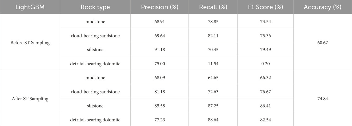
Table 3. Impact of ST composite sampling on classification performance of the LightGBM model.

4.2 ST-ARO-LightGBM model performance

The training effectiveness of the LightGBM model depends on the influence of multiple input hyperparameters. Therefore, the ARO algorithm was employed to find the optimal hyperparameter combination for the LightGBM model. The main hyperparameters and their default values are listed in Table 4. This study simultaneously optimized 7 hyperparameters of the model, where the first three parameters affect the ensemble process of the LightGBM model, and the remaining four parameters influence the process of generating weak classifiers. The ARO algorithm was set with a population size of 50, with each “artificial rabbit” containing 7 hyperparameters. The F1 score of the LightGBM model was used as the fitness value, and the maximum number of iterations was set to 50.

Table 4

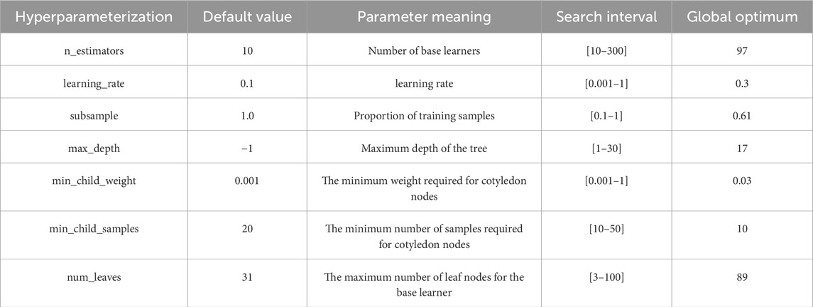
Table 4. Main hyperparameters of the LightGBM model.

Figure 6 shows the change in F1 score during the iteration process with the blue line, while the yellow baseline represents the F1 score trained with default parameters. After 21 iterations, the F1 score stabilized at 81.06%, which is a 3.08% improvement compared to the baseline. After the iteration, the optimal hyperparameter combination of the model is found, and the global optimal solution is shown in the last column of Table 4. At this point, the optimal model contains 97 decision trees, the maximum depth of the trees is 17, the minimum weight to control the splitting of leaf nodes is 0.03, the minimum sample number is 10, and the maximum number of leaf nodes in each decision tree is 89. The proportion of training samples is 0.61, and the learning rate of the model is 0.3.

Figure 6

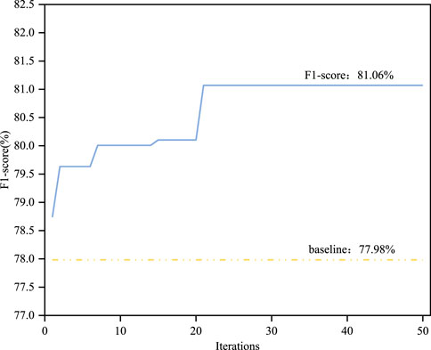
Figure 6. The change of F1 value of ST-ARO-LightGBM identification lithology with the number of iterations.

After dividing the dataset following ST sampling into training and testing sets in a 7:3 ratio, the ST-ARO-LightGBM lithology recognition model was established using AC, CNL, DEN, GR, RT, RXO, T_2LM, POR eight curves, and the optimal hyperparameter combination as inputs. Table 5 shows the classification performance of the proposed model on different lithologies. The classification accuracy on the test set is 81.25%, with F1 scores for the four lithologies being 70.21%, 79.35%, 87.62%, and 87.10% respectively, averaging 81.07%. Compared to the untuned ST-LightGBM model (Table 3), precision, recall, F1 score, and accuracy have improved by 2.99%, 3.15%, 3.09%, and 6.41%, respectively, demonstrating that the ARO algorithm effectively enhances various evaluation metrics of the LightGBM model.

Table 5

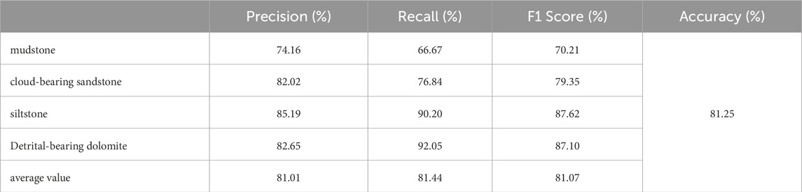
Table 5. Performance of the ST-ARO-LightGBM model for the identification of different lithologies.

5 Discussion

5.1 Model comparison

To verify the lithological classification capabilities of different machine learning models for the Permian shale reservoirs in Jimusar. KNN, DT, XGBoost, GBDT, and RF are several classical machine learning models that have been applied in lithology identification by predecessors (Guo et al., 2003; Ren et al., 2023; Dev and Eden, 2019; Sun Z. et al., 2020; Ahmed and Ali, 2024), but different algorithms have different application effects in different research areas. Therefore, these five algorithms are selected in this paper for comparison.

Table 6 presents a comparison of the classification accuracy and F1 scores of different models before and after ST comprehensive sampling. Before ST sampling, the models achieved an accuracy of 50.56%–72.12% and F1 scores of 36.01%–62.1%. This was because the imbalanced dataset caused the models to overly rely on features from the majority class samples, resulting in low recognition ability for minority class samples and thus weakening the models’ ability to identify lithology.

Table 6

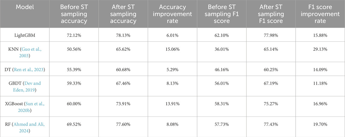
Table 6. Effect of ST integrated sampling on the performance of different models for lithology classification.

After ST comprehensive sampling, the dataset introduced new feature information, leading to a more balanced distribution of samples across various categories. The models could effectively extract features from minority class samples, resulting in an improvement in accuracy by 5.29%–15.06% and F1 scores by 11.18%–29.13%. The LightGBM model performed particularly well with an accuracy of 78.13% and an F1 score of 77.98%. ST comprehensive sampling effectively addressed the issue of dataset imbalance and significantly enhanced the lithological recognition performance of various classifiers, thereby increasing the models’ robustness and applicability.

Due to the overall poor classification performance of the model before ST composite sampling, the ST-ARO-LightGBM model was compared with different models established after sampling. Figure 7 shows the confusion matrices calculated for different models on the test set, visually reflecting the models’ ability to identify various lithologies. The horizontal axis is the true lithology of the sample, the vertical axis is the predicted lithology, and the integer represents the number of samples classified, and the percentage is the corresponding proportion. The darker the color on the main diagonal of the confusion matrix, the better the classification effect on lithology. The ST-ARO-LightGBM model demonstrated the best lithology classification performance, with recognition rates of over 90% for siltstone and detrital-bearing dolomite, and a resolution of 76.84% for cloud-bearing sandstone. However, the resolution for mudstone was relatively low at only 66.67%. This low resolution is due to the interference of logging feature ambiguities, which obscure the differences between mudstone and other lithologies. Other models also exhibited similar characteristics, with the lowest performance seen in the ST-DT model, which had a classification accuracy of only 43.43% for mudstone. This indicates that the proposed ST-ARO-LightGBM model can effectively reduce the interference of weak differences in logging features between different lithologies. To address the issue of low recognition accuracy for mudstone, future research should include more samples to explore the differences between mudstone and other lithologies.

Figure 7

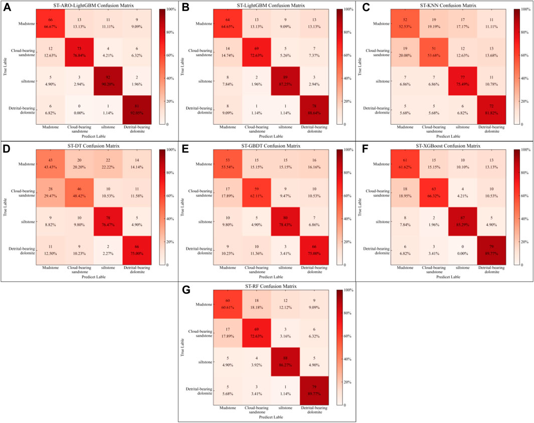
Figure 7. Comparison of confusion matrix for lithology identification by different models. (A) ST-ARO-LightGBM. (B) ST-LightGBM. (C) ST-KNN. (D) ST-DT. (E) ST-GBDT. (F) ST-XGBoost. (G) ST-RF.

Table 7 presents the accuracy, precision, recall, and F1 score of the ST-ARO-LightGBM model and six other models. Through comparative analysis, the ST-ARO-LightGBM model proposed in this study outperforms the other six models in all metrics, consistently achieving over 80%. Combined with Table 7 and Figure 7, the ST-ARO-LightGBM model demonstrates high accuracy and stability in predicting four different lithologies. Compared to traditional machine learning algorithms, it exhibits better robustness and application prospects.

Table 7

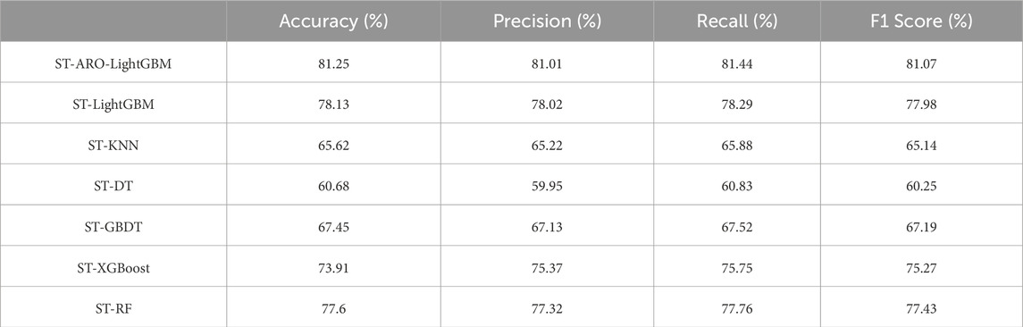
Table 7. Evaluation metrics table of lithology identification by model method after ST sampling.

The results show that the prediction result of integrated machine learning model (such as LightGBM) is better than that of single machine learning model (such as DT and KNN). In addition, the LightGBM model can achieve higher accuracy after being optimized by ARO algorithm, and the performance of machine learning model can be deeply explored, but the iteration time is increased. In the actual modeling process, attention should be paid to the balance between accuracy and computing power, and iteration can be ended in advance within the acceptable accuracy range to achieve the highest accuracy as possible.

5.2 Model application example

To verify the application of the ST-ARO-LightGBM model in the study area, predictions were made for well sections containing different lithologies, as shown in Figures 8, 9. In these figures, the first panel displays depth, the second to fourth panels show input parameters for the model, the fifth panel presents lithological information from rock thin sections not used in model building, the sixth panel shows the lithology predictions and errors of the ST-ARO-LightGBM model, and the seventh to twelfth panels compare the lithology predictions and errors of other models.

Figure 8

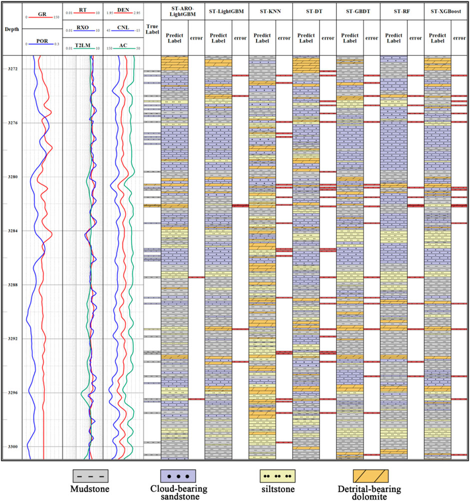
Figure 8. Comparison of lithology of real thin section of rock in well A17X with the lithology identification results of the model proposed in this paper.

Figure 9

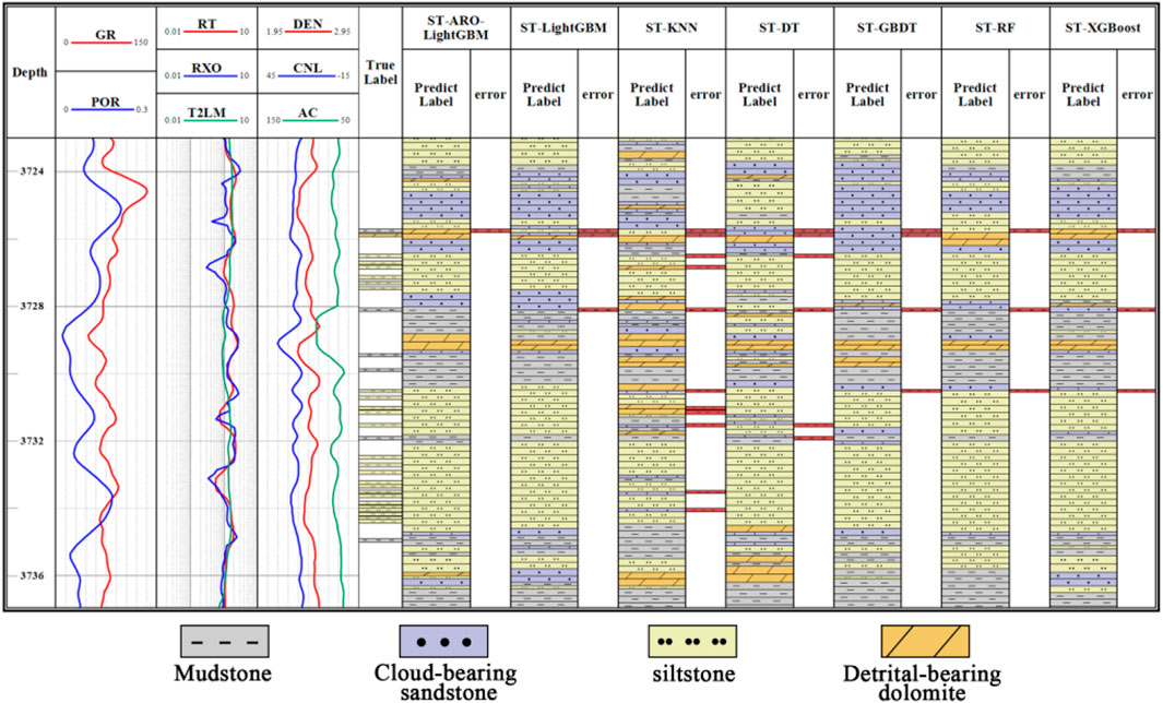
Figure 9. Comparison of lithology of real thin section of rock in well A32X with the lithology identification results of the model proposed in this paper.

Figure 8 illustrates the prediction results for well section A17X from 3,272 to 3,300 m, where mudstone and cloud-bearing sandstone are predominantly developed, with lesser occurrences of siltstone and detrital-bearing dolomite. Through comparison with actual rock thin section lithologies, the ST-ARO-LightGBM model significantly outperforms the six comparison models, accurately reflecting the complex interactions between different lithologies in the actual formations. Errors in the proposed model mainly occur in thin mudstone layers, consistent with the results in Table 5 and Figure 7.

Figure 9 displays the prediction results for well section A32X from 3,724 to 3,736 m, where siltstone and mudstone are primarily developed. The predictions of the ST-ARO-LightGBM model closely match the actual rock thin section lithologies, whereas the comparison models generally capture the variation trends in lithology within the well section but with higher errors.

6 Conclusion

Based on comprehensive experimental results on Permian shale reservoir lithology identification in Jimusaer, the following main conclusions are drawn:

(1) The Permian shale reservoir in Jimusaer primarily consists of mudstone, siltstone, cloud-bearing sandstone, and detrital-bearing dolomite. These lithologies coexist within the actual formations with similar logging response characteristics, posing challenges for traditional lithology identification methods.

(2) The ST composite sampling method effectively enhances the information of minority class samples while reducing redundant information from majority class samples, achieving balanced sample data. This process significantly improves the machine learning model’s performance in lithology prediction tasks and enhances the model’s classification performance and robustness.

(3) By integrating the multi-objective optimization strategy ARO algorithm with the ST-LightGBM model to establish the ST-ARO-LightGBM model, this study efficiently addresses the complex parameter adjustment issues of the ST-LightGBM model, optimizes the model structure, and enhances the lithology prediction capability and applicability of the model.

Although the model proposed in this paper can distinguish different lithologies of shale reservoirs to a certain extent, improve the unbalanced sample set, improve the lithology identification accuracy, and has certain universality, it will increase the calculation time cost due to the need for multiple iterations in the process of model establishment. In addition, the comprehensive analysis of multi-source and multi-modal data has become a research hotspot in the field of artificial intelligence. In future research, on the one hand, we can focus on improving the performance of the machine learning model itself, and on the other hand, we can combine various types of logs data for comprehensive evaluation and analysis.

Data availability statement

The data analyzed in this study is subject to the following licenses/restrictions: The data sets in this study are restricted due to privacy concerns and are not publicly available. Requests to access these datasets should be directed to Cheng Feng, ZmN2aXAwODA4QDEyNi5jb20=.

Author contributions

XD: Investigation, Project administration, Resources, Supervision, Writing–review and editing. JL: Conceptualization, Investigation, Methodology, Project administration, Supervision, Validation, Writing–review and editing. JC: Data curation, Software, Validation, Visualization, Writing–original draft. CF: Conceptualization, Data curation, Formal Analysis, Funding acquisition, Project administration, Resources, Software, Writing–review and editing.

Funding

The author(s) declare that financial support was received for the research, authorship, and/or publication of this article. National Natural Science Foundation of China (No. 42364007, 42004089), the Natural Science Foundation of Xinjiang Uygur Autonomous Region (No. 2021D01E22), the Innovative Outstanding Young Talents of Karamay, Key Research and Development Projects of Xinjiang Uygur Autonomous Region (2024B01016, 2024B01016-1, 2024B01016-3).

Conflict of interest

Authors XD and JL were employed by PetroChina.

The remaining authors declare that the research was conducted in the absence of any commercial or financial relationships that could be construed as a potential conflict of interest.

Generative AI statement

The author(s) declare that no Generative AI was used in the creation of this manuscript.

Publisher’s note

All claims expressed in this article are solely those of the authors and do not necessarily represent those of their affiliated organizations, or those of the publisher, the editors and the reviewers. Any product that may be evaluated in this article, or claim that may be made by its manufacturer, is not guaranteed or endorsed by the publisher.

References

Ahmed, I. B., and Ali, M. A. (2024). Random forest and decision tree facies classification models for well log data of the mishrif formation from Basrah Oil Company, Southern Iraq. Iraqi Geol. J. 57 (2E), 1–15. doi:10.46717/igj.57.2E.2ms-2024-11-11

CrossRef Full Text | Google Scholar

Al-Anazi, A. A., and Gates, I. D. (2010). On the capability of support vector machines to classify lithology from well logs. Nat. Resour. Res. 19, 125–139. doi:10.1007/s11053-010-9118-9

CrossRef Full Text | Google Scholar

Baisakhi, D., and Rima, C. (2018). Well log data analysis for lithology and fluid identification in Krishna-Godavari Basin, India. Arabian J. Geosciences 11, 1–12. doi:10.1007/s12517-018-3587-2

CrossRef Full Text | Google Scholar

Bestagini, P., Vincenzo, L., and Stefano, T. (2017). “A machine learning approach to facies classification using well logs,” in Seg technical program expanded abstracts 2017. Society of Exploration Geophysicists, 2137–2142.

Google Scholar

Bressan, T. S., de Souza, M. K., Girelli, T. J., and Junior, F. C. (2020b). Evaluation of machine learning methods for lithology classification using geophysical data. Comput. and Geosciences 139, 104475. doi:10.1016/j.cageo.2020.104475

CrossRef Full Text | Google Scholar

Bressan, T. S., Kehl de Souza, M., Girelli, T. J., and Junior, F. C. (2020a). Evaluation of machine learning methods for lithology classification using geophysical data. Comput. and Geosciences 139, 104475. doi:10.1016/j.cageo.2020.104475

CrossRef Full Text | Google Scholar

Chen, J., Deng, X., Shan, X., Feng, Z., Zhao, L., Zong, X., et al. (2024). Intelligent classification of volcanic rocks based on honey badger optimization algorithm enhanced Extreme gradient boosting tree model: a case study of hongche fault zone in Junggar Basin. Processes 12 (2), 285. doi:10.3390/pr12020285

CrossRef Full Text | Google Scholar

Chioma, O., Uko, E. D., and Tamunobereton-ari, I. (2018). Determination of lithology and pore-fluid of A reservoir in parts of Niger Delta using well-log data. J. Appl. Phys. 10 (2), 71–82. doi:10.9790/4861-1002017182

CrossRef Full Text | Google Scholar

Deng, S., Pan, H., Li, C., Yan, X., Wang, J., Shi, L., et al. (2023). A real-time lithological identification method based on SMOTE-Tomek and ICSA optimization. Acta Geol. Sinica-English Ed. 98, 518–530. doi:10.1111/1755-6724.15144

CrossRef Full Text | Google Scholar

Dev, V. A., and Eden, M. R. (2019). Formation lithology classification using scalable gradient boosted decision trees. Comput. and Chem. Eng. 128, 392–404. doi:10.1016/j.compchemeng.2019.06.001

CrossRef Full Text | Google Scholar

Devi, D., and Purkayastha, B. (2017). Redundancy-driven modified Tomek-link based undersampling: a solution to class imbalance. Pattern Recognit. Lett. 93, 3–12. doi:10.1016/j.patrec.2016.10.006

CrossRef Full Text | Google Scholar

Feng, C., Feng, Z., Mao, R., Li, G., Zhong, Y., and Ling, K. (2023). Prediction of vitrinite reflectance of shale oil reservoirs using nuclear magnetic resonance and conventional log data. Fuel 339, 127422. doi:10.1016/j.fuel.2023.127422

CrossRef Full Text | Google Scholar

Feng, C., Yang, Z., Feng, Z., Zhong, Y., and Ling, K. (2020). A novel method to estimate resistivity index of tight sandstone reservoirs using nuclear magnetic resonance logs. J. Nat. Gas Sci. Eng. 79, 103358. doi:10.1016/j.jngse.2020.103358

CrossRef Full Text | Google Scholar

Feng, C., Zhong, Z., Mao, Z., Ling, K., and Ling, K. (2021). Determination of reservoir wettability based on resistivity index prediction from core and log data. J. Petroleum Sci. Eng. 205, 108842. doi:10.1016/j.petrol.2021.108842

CrossRef Full Text | Google Scholar

Guo, G., Wang, H., Bell, D., Bi, Y., and Greer, K. (2003). KNN model-based approach in classification[C]//On the move to meaningful internet systems 2003: CoopIS, DOA, and ODBASE: OTM confederated international conferences, CoopIS, DOA, and ODBASE 2003, Catania, Sicily, Italy. Berlin, Heidelberg: Springer, 986–996.

Google Scholar

Han, R., Wang, Z., Zhang, Z., Wang, X., Cui, Y., and Guo, Y. (2024). Prediction of igneous lithology and lithofacies based on ensemble learning with data optimization. Geophysics 89 (2), 1–JM11. doi:10.1190/geo2022-0782.1

CrossRef Full Text | Google Scholar

Huang, A., Cai, W., Wei, X., Li, Y., Duan, G., and Liu, D. (2023). Lithology identification of volcanic logging based on improved random forest. Sci. Technol. Eng. 23 (09), 3696–3704.

Google Scholar

Imamverdiyev, Y., and Lyudmila, S. (2019). Lithological facies classification using deep convolutional neural network. J. Petroleum Sci. Eng. 174, 216–228. doi:10.1016/j.petrol.2018.11.023

CrossRef Full Text | Google Scholar

Ke, G., Meng, Q., Finley, T., Wang, T., Chen, W., Ma, W., et al. (2017). Lightgbm: a highly efficient gradient boosting decision tree. Adv. neural Inf. Process. Syst., 30. doi:10.5555/3294996.3295074

CrossRef Full Text | Google Scholar

Li, Q., Peng, C., Fu, J., Xiaomin, Z., Yu, S., Chengxu, Z., et al. (2023). A comprehensive machine learning model for lithology identification while drilling. Geoenergy Sci. Eng. 231, 212333. doi:10.1016/j.geoen.2023.212333

CrossRef Full Text | Google Scholar

Mitchell, J. (2020). Monitoring lithology variations in drilled rock formations using NMR apparent magnetic susceptibility contrast. Appl. Magn. Reson. 51 (3), 205–219. doi:10.1007/s00723-019-01157-1

CrossRef Full Text | Google Scholar

Mou, D., Zhang, L., and Xu, C. (2021). Comparison of three classical machine learning algorithms for lithology identification of volcanic rocks using well logging data. J. Jilin Univ. Sci. Ed. 51 (03), 951–956. doi:10.13278/j.cnki.jjuese.20200210

CrossRef Full Text | Google Scholar

Passey, Q. R., Bohacs, K. M., Esch, W. L., Klimentidis, R., and Sinha, S. (2010). “From oil-prone source rock to gas-producing shale reservoir–geologic and petrophysical characterization of unconventional shale-gas reservoirs,” in SPE International oil and gas Conference and exhibition in China. SPE.

Google Scholar

Pereira, R. M., Costa, Y. M. G., and Silla, Jr C. N. (2020). MLTL: a multi-label approach for the Tomek Link undersampling algorithm. Neurocomputing 383, 95–105. doi:10.1016/j.neucom.2019.11.076

CrossRef Full Text | Google Scholar

Prabowo, U. N., Ferdiyan, A., Raharjo, S. A., Sehah, S., and Candra, A. D. (2023). Comparison of facies estimation using support vector machine (SVM) and K-nearest neighbor (KNN) algorithm based on well log data. Aceh Int. J. Sci. Technol. 12 (2), 246–253. doi:10.13170/aijst.12.2.28428

CrossRef Full Text | Google Scholar

Probst, P., Anne-Laure, B., and Bernd, B. (2019). Tunability: importance of hyperparameters of machine learning algorithms. J. Mach. Learn. Res. 20 (53), 1–32. doi:10.48550/arXiv.1802.09596

CrossRef Full Text | Google Scholar

Ren, Q., Zhang, H., Zhang, D., and Zhao, X. (2023). Lithology identification using principal component analysis and particle swarm optimization fuzzy decision tree. J. Petroleum Sci. Eng. 220, 111233. doi:10.1016/j.petrol.2022.111233

CrossRef Full Text | Google Scholar

Saporetti, C. M., Goliatt, L., and Pereira, E. (2021). Neural network boosted with differential evolution for lithology identification based on well logs information. Earth Sci. Inf. 14, 133–140. doi:10.1007/s12145-020-00533-x

CrossRef Full Text | Google Scholar

Saporetti, C. M., Leonardo Goliatt da, F., and Egberto, P. (2019). A lithology identification approach based on machine learning with evolutionary parameter tuning. IEEE Geoscience Remote Sens. Lett. 16 (12), 1819–1823. doi:10.1109/lgrs.2019.2911473

CrossRef Full Text | Google Scholar

Sebtosheikh, M. A., Motafakkerfard, R., Riahi, M. A., Moradi, S., and Sabety, N. (2015). Support vector machine method, a new technique for lithology prediction in an Iranian heterogeneous carbonate reservoir using petrophysical well logs. Carbonates evaporites 30, 59–68. doi:10.1007/s13146-014-0199-0

CrossRef Full Text | Google Scholar

Singh, A., and Maheswar, O. (2022). Machine learning in the classification of lithology using downhole NMR data of the NGHP-02 expedition in the Krishna-Godavari offshore Basin, India. Mar. Petroleum Geol. 135, 105443. doi:10.1016/j.marpetgeo.2021.105443

CrossRef Full Text | Google Scholar

Sun, Y., Huang, Y., Liang, T., Ji, H., Xiang, P., and Xu, X. (2020a). Identification of complex carbonate lithology by logging based on XGBoost algorithm. Lithol. Reserv. 32 (04), 98–106. doi:10.12108/yxyqc.20200410

CrossRef Full Text | Google Scholar

Sun, Z., Jiang, B., Li, X., Li, J., and Xiao, K. (2020b). A data-driven approach for lithology identification based on parameter-optimized ensemble learning. Energies 13 (15), 3903. doi:10.3390/en13153903

CrossRef Full Text | Google Scholar

Thongsamea, W., Kanitpanyacharoena, W., and Chuangsuwanich, E. (2021). Lithological classification from well logs using machine learning algorithms. Bull. Earth Sci. Thail. 10 (1), 31–43.

Google Scholar

Wang, L., Cao, Q., Zhang, Z., Mirjalili, S., and Zhao, W. (2022). Artificial rabbits optimization: a new bio-inspired meta-heuristic algorithm for solving engineering optimization problems. Eng. Appl. Artif. Intell. 114, 105082. doi:10.1016/j.engappai.2022.105082

CrossRef Full Text | Google Scholar

Wang, Q., Yang, T., Liu, Y., Nie, X., Zhang, Z., and Wan, Y. (2020). Identification of complex carbonate lithology based on random forest algorithm. Chin. J. Eng. Geophys. 17 (05), 550–558. doi:10.3969/j.issn.1672-7940.2020.05.003

CrossRef Full Text | Google Scholar

Xiong, X., Xiao, D., Lei, X., Li, Y., Lu, S., Wang, M., et al. (2023). Response of well logging and “sweet spot” rapid evaluation technology for shale oil in the Lucaogou Formation of Jimsar Sag. Special Oil and Gas Reservoirs 30 (04), 35–43. doi:10.3969/j.issn.1006-6535.2023.04.005

CrossRef Full Text | Google Scholar

Zha, X. (2022). Characteristics and classification evaluation of shale oil reservoir of the Lucaogou Formation in Jimsa. (Dissertation). Chongqing University of Science and Technology.

Google Scholar

Zou, C., Yang, Z., Zhu, R., Zhang, G., Hou, L., Wu, S., et al. (2015). Progress in China's unconventional oil and gas exploration and development and theoretical technologies. Geol. Rev. 89 (06), 979–1007. doi:10.1111/1755-6724.12491

CrossRef Full Text | Google Scholar