A transformer-based method for correcting daily SST numerical forecasting products

This study introduces applies a Transformer-based method to correct daily Sea Surface Temperature (SST) numerical forecasting products, addressing persistent challenges in short-term SST prediction. The proposed approach utilizes a Transformer model architecture to capture complex spatiotemporal dependencies in SST error fields, enabling efficient prediction of forecast errors across multiple time scales. The method was applied to SST hindcast data from the First Institute of Oceanography (FIO-COM) ocean forecasting system, focusing on the northwestern Pacific region. Results demonstrate significant improvements in forecast accuracy, with Root Mean Square Error (RMSE) reductions ranging from 38.8% for day 2 forecasts to 17.6% for day 5 forecasts. Spatial analysis reveals the method’s robust performance across diverse oceanographic regimes, including complex coastal and shelf regions where traditional models often struggle. The Transformer model showed the ability to capture and reproduce error patterns, effectively addressing both large-scale systematic biases and smaller-scale regional variations. The consistent performance across different forecast horizons suggests potential for extending the reliable forecast range of SST predictions. The findings have important implications for applications requiring precise SST forecasts, including operational oceanography, marine weather forecasting, and coupled ocean-atmosphere modeling.

1 Introduction

SST plays a pivotal role in the Earth’s climate system, serving as a fundamental parameter in the complex interactions between the ocean and atmosphere (Deser et al., 2010). Accurate SST forecasts, particularly within the short-term range, are crucial for a wide array of applications, including weather prediction, marine operations, fisheries management, and coastal ecosystem monitoring (Schade, 2000; Planque et al., 2003; Kessler et al., 2022). The importance of daily SST forecasts has grown significantly in recent years, driven by the increasing demand for high-resolution, timely oceanographic information in various sectors (Xie et al., 2024; Patil and Deo, 2017).

Current SST numerical forecasting methods for short-term predictions have evolved continuously, leveraging complex ocean models that incorporate a diverse array of physical processes (Chassignet et al., 2009; Wei et al., 2016; O’dea et al., 2012). These include heat fluxes at the air-sea interface, three-dimensional ocean currents, vertical and horizontal mixing processes, and thermohaline stratification (Busecke et al., 2024; Ferrari et al., 2008; Bennis et al., 2020; de et al., 2020). The accuracy of these models has been greatly enhanced by advancements in computational resources, allowing for higher spatial and temporal resolutions, as well as the inclusion of more sophisticated physical parameterizations (Zhu and Zhang, 2019). Furthermore, the integration of improved data assimilation techniques, such as ensemble Kalman filters and variational methods, has boosted forecast skill by optimally combining observational data with model predictions (Belyaev et al., 2021). Recent developments also include the incorporation of coupled atmosphere-ocean models and the assimilation of satellite-derived SST data, leading to more accurate representations of air-sea interactions and improved forecast accuracy (Miller et al., 2017; Manda et al., 2005).

Despite significant advancements, achieving high-accuracy daily SST forecasts within the short-term range using numerical models remains challenging (Barton et al., 2021). Persistent issues include model biases, insufficient spatial resolution to capture mesoscale features, and uncertainties in air-sea flux parameterizations (Fyfe et al., 2021). The complex dynamics of coastal regions and the impact of sub-mesoscale processes pose significant difficulties (Stanev et al., 2020). While the integration of satellite data and in-situ observations through advanced data assimilation techniques has improved forecast accuracy, gaps in observational coverage and data quality issues continue to limit progress (de et al., 2022). Addressing these challenges requires ongoing research in model physics, data assimilation methods, and observational techniques to enhance the reliability of daily SST forecasts.

In recent years, machine learning (ML) techniques have shown great promise in complementing and enhancing traditional numerical weather prediction (NWP) methods for SST forecasting (Sarkar et al., 2020). ML approaches offer several potential advantages, including the ability to capture complex, non-linear relationships in oceanic and atmospheric processes (Ali et al., 2021). These methods can efficiently assimilate and process vast amounts of heterogeneous data from satellites, buoys, and numerical models (Elafi et al., 2024; Zrira et al., 2024; Yu et al., 2020; Shao et al., 2021). Additionally, ML algorithms have demonstrated skill in reducing systematic biases and improving forecast accuracy across various temporal and spatial scales. The integration of ML with physics-based models through hybrid approaches shows particular promise in leveraging the strengths of both paradigms, potentially leading to more accurate and computationally efficient SST forecasts (Fei et al., 2022).

The Transformer model, introduced by Vaswani (2017), has advanced the field of natural language processing and demonstrates promising potential for SST forecasting (Alerskans et al., 2022). This architecture offers several advantages, including bias correction capabilities, an attention mechanism for identifying relevant patterns, the ability to capture long-range dependencies, efficient parallelization, and scalability (Dai et al., 2024; Zou et al., 2023). Recent advancements in interpretability techniques further enhance its potential for providing insights into SST dynamics (Zhou and Zhang, 2023). Meng and Hakim (2024) utilized a Transformer-based model to reconstruct the upper ocean of the tropical Pacific through online data assimilation, demonstrating superior performance over traditional methods in handling sparse, high-noise observational data and improving forecast accuracy. Agabin et al. (2024) proposed an NLP-inspired algorithm, combined with high-fidelity ocean simulations, capable of reconstructing missing SST data with an RMSE of ≲0.1K. Additionally, Goh et al. (2024) introduced a deep learning-based Masked Autoencoder (MAE) method, which efficiently fills missing data by learning ocean frontal features, significantly reducing reconstruction errors and improving computational efficiency by three orders of magnitude compared to traditional methods.

The present study proposes a Transformer-based method for correcting daily SST numerical forecasts, with the aim of enhancing accuracy and reliability. This approach involves training the model on historical numerical hindcast SST datasets in con-junction with corresponding observational data. The evaluation will be conducted using comprehensive metrics across extended time series and case studies. In the following sections, we will detail the method, including the data preprocessing steps, model architecture, training procedure, and evaluation metrics. We will then present the results of our experiments, discuss the implications of our findings, and conclude with suggestions for future research directions in this promising field of ML-enhanced SST forecasting.

2 Data and method

2.1 Data

The SST hindcast data utilized in this study is derived from an advanced ocean forecasting system specifically designed for the 21st-Century Maritime Silk Road (Qiao et al., 2019). This system (FIO-COM) was developed by the First Institute of Oceanography, Ministry of Natural Resources, China, and integrates complex interactions between waves, tides, and circulation patterns, providing a comprehensive representation of marine processes. Its operational launch on 10 December 2018 represented a advancement in China’s ability to model and forecast oceanic conditions.

The dataset employed in this research spans from the system’s inception date, 10 December 2018, to 31 December 2023, providing a comprehensive temporal range for daily SST forecasting error correction analysis. The hindcast process within this system is executed daily at 12:00 UTC, ensuring a consistent and continuous data stream. Data up-dates occur at 3-h intervals, with a spatial resolution of 0.1 ° × 0.1 °. Based on this high-resolution output, daily SST forecasts have been computed.

While the model is capable of global coverage, our study strategically focuses on the northwestern Pacific region, defined by the coordinates 100°E to 145°E and 0°S to 45°N. This delineation optimizes computational efficiency and resource management while encompassing an area of critical importance for China. The selected region includes all Chinese coastal areas, characterized by intense marine economic activities, where accurate environmental forecasting is crucial for safe and efficient operations.

For observational comparison, we employ the Group for High Resolution Sea Surface Temperature (GHRSST) global Level 4 SST analysis, produced daily on a 0.25-degree grid by remote sensing systems. This product utilizes optimal interpolation (OI) from multiple microwave (MW) sensors, including the Global Precipitation Measurement (GPM) Microwave Imager (GMI), the Tropical Rainfall Measuring Mission (TRMM) Microwave Imager (TMI), NASA’s Advanced Microwave Scanning Radiometer-EOS (AMSRE), the Advanced Microwave Scanning Radiometer 2 (AMSR2) onboard the GCOM-W1 satellite, and WindSat on the Coriolis satellite. The through-cloud capabilities of these microwave radiometers provide a robust and comprehensive representation of global SST patterns.

To maintain consistency with the numerical forecasting products, we interpolate the observed SST data to match the grid of the forecasting SST. This allows for direct comparison and error calculation by subtracting the observed SST from the corresponding fore-casted SST. The resulting error fields for each forecasting case form the foundation for SST error training and evaluation.

The accuracy of numerical SST forecasting at different prediction horizons (day 2 to day 5) is influenced by multiple factors, including inaccuracies in the representation of physical processes, errors in air-sea fluxes, and uncertainties in model initial conditions. However, our investigation reveals a significant correlation between errors at different forecasting periods and those present in the initial conditions. This observation motivates our approach to construct a relationship between model errors on the first day and fore-casting errors at subsequent time steps using transformer-based methods.

After training on historical datasets, we develop transformer-based models capable of predicting forecasting errors for days 2–5 based on the errors observed on day 1. Given that the completion of a full forecast typically lags real-time by approximately 1 day, the model errors for day 1 can be calculated using available observations. Subsequently, the predicted errors can be subtracted from the numerical forecasting products, thereby enhancing the model’s forecasting accuracy for daily SST across different prediction horizons. This method represents an approach to improving SST forecasting accuracy by leveraging advanced machine learning techniques in conjunction with traditional numerical modeling. The integration of these methods is expected to effectively enhance our ability to predict SST patterns in the northwestern Pacific region, further supporting maritime activities and environmental monitoring in the area, delivering significant practical value.

2.2 Method

2.2.1 SST error prediction transformer methods

This study proposes a Transformer-based prediction model specifically de-signed for SST error fields. Our approach builds upon Zhou’s model for analyzing three-dimensional ocean thermal distributions (Zhou and Zhang, 2023) and Kang’s method for correcting wave significant forecasting errors (Kang et al., 2024). The adapted Transformer model primarily focuses on predicting SST error fields at different forecasting periods by leveraging the global feature extraction capabilities of the Transformer architecture.

The SST error prediction system consists of four independently trained Transformer models, with each model specifically trained for predicting errors at a different forecast day (Figure 1). We trained Model one to predict day 2 errors, Model two for day 3 errors, Model three for day 4 errors, and Model four for day 5 errors, with all models using day 1 error fields as input. Each model was trained separately with its corresponding target day’s error data to optimize performance for that specific forecast period. After prediction, the error fields generated by these four models are subtracted from their respective day’s SST forecasts to obtain the corrected SST fields. This distinct model approach ensures that each forecast day’s unique error characteristics are captured by a dedicated model.

Figure 1

Figure 1. The workflow of the SST error prediction.

The SST error prediction and correction capability is grounded in the core Trans-former model, which maintains a consistent architectural structure. This core Transformer model employs an encoder-decoder framework that consists of two overlapping decom-position modules, two embedding modules, an encoder module, a decoder module, and a linear output module (Figure 2a).

Figure 2

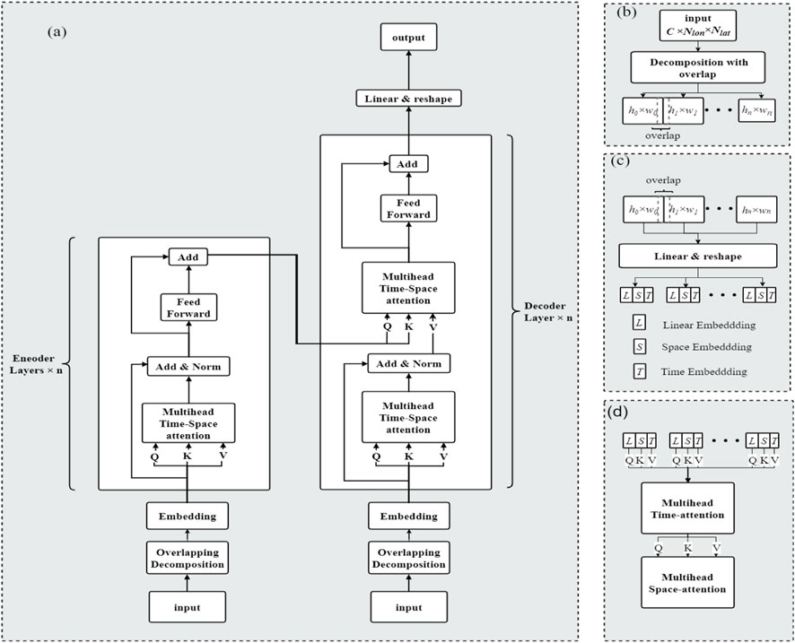
Figure 2. Architecture of the Transformer model for SST error prediction. (a) Model Overview: Shows the encoder-decoder structure. (b) Decomposition with Overlap modules: Segments the SST error field into patches. (c) Embedding Module: Adds linear, spatial, and temporal embeddings. (d) Attention Mechanism: Uses multi-head attention for spatial and temporal patterns.

To address the issue of information fragmentation between the edges of patches and adjacent patches, which affects the overall continuity of SST predicted error fields, overlapping decomposition modules are positioned prior to the embedding layer, as depicted in Figure 2b. The operation of these modules commences with the acceptance of the input SST error field for day 1, represented as ${\mathit{X}}_{{\mathit{T}}_{\mathit{i}\mathit{n}}\times {\mathit{N}}_{\mathit{l}\mathit{a}\mathit{t}}\times {\mathit{N}}_{\mathit{l}\mathit{o}\mathit{n}}}^{\mathit{i}\mathit{n}}$ which are dimensioned at $T_{in}\times N_{lat}\times N_{lon}=1\times 225\times 225$. Subsequently, each set of inputs is partitioned using a sliding strategy from left to right and top to bottom, resulting in $N$ fixed-size patches ${\mathit{X}}_{{\mathit{T}}_{\mathit{i}\mathit{n}}\times \mathit{N}\times \left(\mathit{h}\times \mathit{w}\right)}^{\mathit{i}\mathit{n}}$, where $N=\left(\frac{N_{lat}}{h}\right)\times \left(\frac{N_{lon}}{w}\right)$ represents the total count of decomposed patches, each patch measures $h\times w=9\times 9$ (where $h$​ and $w$​ represent the number of grid points in the height and width of the overlapping blocks, respectively), with an overlap size of three between the patches.

Two embedding modules transform the decomposed inputs ${\mathit{X}}_{{\mathit{T}}_{\mathit{i}\mathit{n}}\times \mathit{N}\times \left(\mathit{h}\times \mathit{w}\right)}^{\mathit{i}\mathit{n}}$ into more expressive feature representations by employing various embedding techniques, including linear, time, and space embeddings (Figure 2c), which capture complex patterns across both time and space.

The linear embedding transforms the inputs into more expressive feature vectors ${\mathit{X}}_{{\mathit{T}}_{\mathit{i}\mathit{n}}\times \mathit{N}\times \mathit{d}}^{\mathit{l}}$, with the embedding dimension set to $d=512$. The formula for the linear embedding is shown in Equation 1:

$\mathit{y}=\mathit{W}\mathit{x}+\mathit{b}(1)$

Where $\mathit{x}$ is the decomposed input data, $\mathit{W}$ is the weight matrix for the linear transformation, and $\mathit{b}$ is the bias vector.

In the time embedding process, a zero-initialized positional encoding matrix ${\mathit{P}\mathit{E}}_{\mathit{t}\mathit{i}\mathit{m}\mathit{e}}={\mathit{X}}_{{\mathit{T}}_{\mathit{i}\mathit{n}}\times \mathbf{1}\times \mathit{d}}^{\mathit{t}}$ is first initialized based on the shape of the input data, with its length corresponding to the temporal dimension $T_{in}$. Subsequently, the temporal positional encoding function is applied to encode the data at each time step, and the resulting encoded values are filled into the corresponding positions of the temporal positional encoding matrix. The formulas for temporal positional encoding and spatial attention are shown in Equations 2, 3, respectively.

$\mathit{P}\mathit{E}\left(tim{e}_{pos},2i\right)=\mathit{sin}\left(\frac{tim{e}_{pos}}{{10000}^{\frac{2i}{d}}}\right)(2)$

$\mathit{P}\mathit{E}\left(tim{e}_{pos},2i+1\right)=\mathit{cos}\left(\frac{tim{e}_{pos}}{{10000}^{\frac{2i+1}{d}}}\right)(3)$

Where $tim{e}_{pos}$ represents the position of the current data in the temporal dimension for the $2i$ or $2i+1$ region, $d=512$ is the feature dimension, $2i$ represents the even dimensions of the regional data, and $2i+1$ represents the odd dimensions.

In the space embedding process, an embedding matrix ${\mathit{P}\mathit{E}}_{\mathit{s}\mathit{p}\mathit{a}\mathit{c}\mathit{e}}={\mathit{X}}_{\mathbf{1}\times \mathit{N}\times \mathit{d}}^{\mathit{s}}$ is defined, where $N$ represents the number of spatial positions, and $d=512$ denotes the dimension of the embedding vector. The embedding matrix ${\mathit{P}\mathit{E}}_{\mathit{s}\mathit{p}\mathit{a}\mathit{c}\mathit{e}}$ is initially generated by randomly sampling from a uniform distribution within the interval $\left[-\sqrt{k},\sqrt{k}\right]$, where $k=\frac{1}{d}$. During each training iteration, ${\mathit{P}\mathit{E}}_{\mathit{s}\mathit{p}\mathit{a}\mathit{c}\mathit{e}}$​ is updated according to the learning rat $\eta$ and the gradient of the loss function $\mathrm{L}$. After backpropagation, ${\mathit{P}\mathit{E}}_{\mathit{s}\mathit{p}\mathit{a}\mathit{c}\mathit{e}}$ gradually converge to the optimal solution, effectively capturing spatial dependencies. The update formula is shown in Equation 4:

${\mathit{P}\mathit{E}}_{\mathit{s}\mathit{p}\mathit{a}\mathit{c}\mathit{e}}^{\left(t+1\right)}={\mathit{P}\mathit{E}}_{\mathit{s}\mathit{p}\mathit{a}\mathit{c}\mathit{e}}^{\left(t\right)}-\eta \frac{\mathbf{\partial }\mathbf{L}}{\mathbf{\partial }{\mathit{P}\mathit{E}}_{\mathit{s}\mathit{p}\mathit{a}\mathit{c}\mathit{e}}^{\left(t\right)}}(4)$

where $\frac{\mathbf{\partial }\mathbf{L}}{\mathbf{\partial }{\mathit{P}\mathit{E}}_{\mathit{s}\mathit{p}\mathit{a}\mathit{c}\mathit{e}}^{\left(t\right)}}$ is the gradient of the loss function L with respect to the embedding vector.

Upon receiving the high-dimensional data vectors ${\mathit{X}}_{{\mathit{T}}_{\mathit{i}\mathit{n}}\times \mathit{N}\times \mathit{d}}={\mathit{X}}_{{\mathit{T}}_{\mathit{i}\mathit{n}}\times \mathit{N}\times \mathit{d}}^{\mathit{l}}+{\mathit{X}}_{\mathbf{1}\times \mathit{N}\times \mathit{d}}^{\mathit{s}}+{\mathit{X}}_{{\mathit{T}}_{\mathit{i}\mathit{n}}\times \mathbf{1}\times \mathit{d}}^{\mathit{t}}$, The encoder module commences its analysis (Figure 2d). First, ${\mathit{X}}_{{\mathit{T}}_{\mathit{i}\mathit{n}}\times \mathit{N}\times \mathit{d}}$ is transformed into ${\mathit{X}}_{{\mathit{T}}_{\mathit{i}\mathit{n}}\times {\mathbf{N}}^{\mathit{t}}}^{\mathit{T}}$, where ${\mathbf{N}}^{\mathit{t}}=\mathit{N}\times \mathit{d}$. Then, temporal self-attention is computed using the attention formula. Next, the adjusted data ${\mathit{X}}_{{\mathit{T}}_{\mathit{i}\mathit{n}}\times {\mathbf{N}}^{\mathit{t}}}^{\mathit{T}}$ is mapped to ${\mathit{X}}_{\mathit{N}\times {\mathit{N}}^{\mathit{s}}}^{\mathit{s}}$,where ${\mathbf{N}}^{\mathit{s}}={\mathit{T}}_{\mathit{i}\mathit{n}}\times \mathit{d}$, and spatial self-attention is computed using the attention formula, ultimately generating a feature matrix through a linear transformation. After undergoing $n=4$ iterations of feature extraction within the encoding blocks, the final feature matrix ${\mathit{X}}_{{\mathit{T}}_{\mathit{i}\mathit{n}}\times \mathit{N}\times \mathit{d}}^{\mathit{e}\mathit{n}\mathit{c}\mathit{o}\mathit{d}\mathit{e}-\mathit{o}\mathit{u}\mathit{t}}$ is produced and passed to the subsequent decoder. The attention formula is shown in Equation 5:

$\mathbf{Attention}\left(\mathbf{Q},\mathbf{K},\mathbf{V}\right)=\mathbf{S}\mathbf{o}\mathbf{f}\mathbf{t}\mathbf{M}\mathbf{a}\mathbf{x}\left(\frac{{\mathbf{QK}}^{\mathit{T}}}{\sqrt{\mathit{d}}}\right)\mathbf{V}(5)$

The vectors $\mathbf{Q}$, $\mathbf{K}$, and $\mathbf{V}$ are the query, key, and value vectors generated along the spatiotemporal dimension, respectively, with $\mathit{Q}=\mathit{K}=\mathbf{V}$, and $d=512$ is the feature dimension of $\mathbf{Q}$ ​and $\mathbf{K}$.

The decoder module processes the feature matrix ${\mathit{X}}_{{\mathit{T}}_{\mathit{i}\mathit{n}}\times \mathit{N}\times \mathit{d}}^{\mathit{e}\mathit{n}\mathit{c}\mathit{o}\mathit{d}\mathit{e}-\mathit{o}\mathit{u}\mathit{t}}$ generated by the encoder for analysis. In this process, the decoder uses the encoder’s output as both the query (Q) and the key (K), while the value (V) is computed from the attention calculation based on the decoder’s input. By applying function 5, the decoder effectively integrates the rich feature information extracted by the encoder and passes it to the feedforward neural network for further refinement. After detailed processing through four decoder blocks and the linear output module, the resulting SST error field ${\mathit{X}}_{{\mathit{T}}_{\mathit{o}\mathit{u}\mathit{t}}\times {\mathit{N}}_{\mathit{l}\mathit{a}\mathit{t}}\times {\mathit{N}}_{\mathit{l}\mathit{o}\mathit{n}}}^{\mathit{o}\mathit{u}\mathit{t}}$ maintains consistency in both spatial and temporal resolution with the initial input SST data.

2.2.2 Model training strategy

For model training, we utilized hindcast datasets spanning from 10 December 2018, to 31 December 2022, with datasets from 1 January 2023, to 31 December 2023, reserved for testing. This approach was chosen to systematically evaluate the method’s generalizability and universal applicability, specifically assessing its potential for implementation in daily operational forecasting corrections. Land points are excluded from the calculations, enhancing the model’s ability to capture the spatiotemporal variability of SST errors specifically in oceanic environments. This focused approach improves the overall effectiveness of the analysis in marine settings.

The Huber loss function was employed to quantify the difference between transformer-predicted and actual SST forecasting errors. This loss function is defined in Equation 6:

$Huberloss=\left\{\begin{array}{l}\frac{1}{2}{\mathit{X}}^2,if\left|\mathit{X}\right|\le \theta \\ \theta \left(\left|\mathit{X}\right|-\frac{1}{2}\theta \right),if\left|\mathit{X}\right|>\theta \end{array}\right.(6)$

where, $\mathit{X}$ represents the residual error, calculated as the true value minus the predicted value. For SST prediction, $\mathit{X}$ is in units of degrees Celsius (°C). The parameter $\theta =0.5$ is a threshold used to distinguish between small and large errors, optimizing the model’s performance. The Huber loss function provides robustness against outliers while maintaining sensitivity to smaller errors.

Model optimization involved several key strategies. We implemented weight sharing for consistency and stability across the four Transformer models. The Adam optimizer was employed with an initial learning rate of $1.5\times {10}^{-4}$ , a batch size of 1, an attention dimension of 256, and a feedforward network dimension of 512. To prevent overfitting, we implemented Dropout regularization with a rate of 0.2 and early stopping, halting training if validation performance did not improve over four consecutive epochs.

Model accuracy was assessed using RMSE on the validation set after each training epoch. The RMSE function is defined in Equation 7:

$\text{RMSE}=\frac{1}{{\mathrm{T}}_{\text{out}}}{\displaystyle \sum _{\mathrm{t}=1}^{{\mathrm{T}}_{\text{out}}}}\sqrt{\frac{1}{{\mathrm{N}}_{\text{lat}}\times {\mathrm{N}}_{\text{lon}}}{\displaystyle \sum _{\mathrm{i}=1}^{{\mathrm{N}}_{\text{lon}}}}{\displaystyle \sum _{\mathrm{j}=1}^{{\mathrm{N}}_{\text{lat}}}}{\left({\mathbf{X}}_{\mathbf{t}.\mathbf{j}.\mathbf{i}}^{\mathbf{out}}-{\mathbf{X}}_{\mathbf{t}.\mathbf{j}.\mathbf{i}}^{\mathbf{tg}}\right)}^2}(7)$

where, ${\mathit{X}}^{\mathit{t}\mathit{g}}$ represents the target predictand field, and ${\mathit{X}}^{\mathit{o}\mathit{u}\mathit{t}}$ denotes the output fields. ${\mathrm{T}}_{\text{out}}$​ refers to the forecast time steps, ${\mathrm{N}}_{\text{lat}}$ and ${\mathrm{N}}_{\text{lon}}$ ​denote the number of grid points in the latitude and longitude directions, respectively.

This comprehensive approach to SST error prediction, combining advanced Transformer architectures with rigorous training and evaluation strategies, aims to improve the accuracy and reliability of SST forecasts, addressing key challenges in oceanographic modeling and prediction.

3 Results

Our study aimed to address the persistent challenges in short-term SST forecasting through the application of a Transformer-based correction method. The results presented here demonstrate significant improvements in forecast accuracy across various temporal and spatial scales, addressing key limitations of traditional numerical forecasting approaches.

3.1 Evaluation of correction effects

Figure 3 presents a comparison of the original FIO-COM and corrected SST forecasts for the year 2023, illustrating the improvements achieved through our Transformer-based correction method. This analysis addresses a primary challenge in SST forecasting: maintaining accuracy over different forecast horizons while adapting to varying oceanic conditions. Figure 3a displays the time series of spatially-averaged RMSE for forecast intervals from day 2 to day 5, revealing several insights into the performance of our correction method. Notably, the corrected forecasts demonstrate consistently lower RMSE values compared to the original FIO-COM forecasts across all forecast periods, underscoring the robustness of our Transformer-based approach in mitigating systematic biases inherent in the numerical model. This persistent improvement is particularly significant given the complex and dynamic nature of oceanic systems, which often pose substantial challenges to traditional forecasting methods.

Figure 3

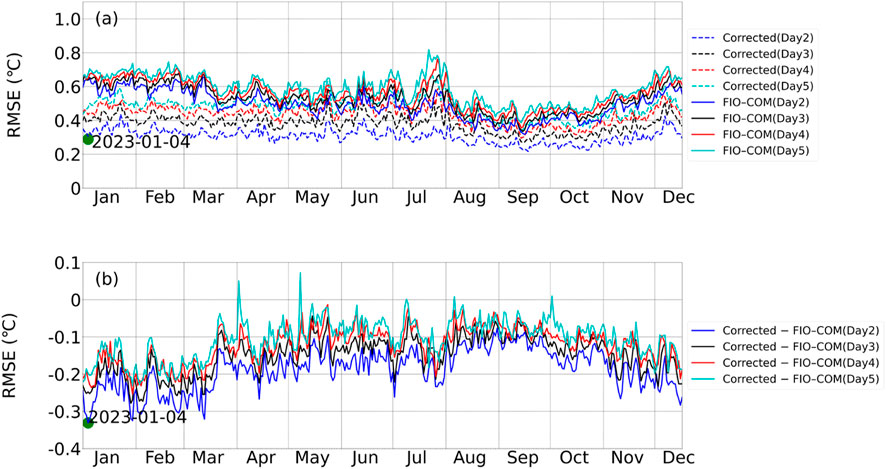
Figure 3. Comparison of original FIO-COM and corrected SST forecasts in 2023. (a) Time series of spatially-averaged RMSE (°C) for day 2 to day 5 forecast intervals (Dashed lines represent corrected RMSE, while solid lines indicate original FIO-COM RMSE). (b) RMSE skill difference between corrected and original SST forecasts (negative values indicate effective correction, while positive values suggest ineffective correction). Different colors represent forecasting results for various lead times. The red dots indicate a specific hindcast case initiated at 1200 UTC 4 January 2023, selected for detailed case analysis.

The temporal variability observed in the RMSE for both original and corrected forecasts throughout the year reflects the dynamic nature of oceanic conditions and their impact on forecast complexity. This adaptability is crucial for real-world applications, where oceanic states can change rapidly and unpredictably. As anticipated, the RMSE generally increases with the forecast horizon for both original and corrected forecasts, aligning with the growing uncertainty in longer-range predictions and the compounding effects of model errors over time. However, the consistent performance of our correction method across all horizons suggests its efficacy in addressing both short-term and long-term forecast challenges, a significant advancement in SST prediction capabilities.

Of particular note is the method’s performance during periods of extreme events or anomalous oceanic conditions, evidenced by several pronounced RMSE spikes in the time series. Our correction method demonstrates effectiveness during these critical periods, reducing the magnitude of these error spikes. This capability is of importance for improving forecast reliability during extreme oceanic events, which can have substantial impacts on marine ecosystems, weather patterns, and human activities in coastal regions. Furthermore, the RMSE exhibits discernible seasonal patterns, with generally higher errors observed during the summer months (approximately July-August). This pattern aligns with the known challenges of forecasting SST during periods of increased stratification and higher variability characteristic of summer months, further highlighting the adaptive nature of our Transformer-based approach.

Figure 3b provides additional insights into the effectiveness of our correction method by illustrating the RMSE skill difference between the corrected and original SST forecasts. The predominantly negative values across all forecast horizons indicate a persistent reduction in forecast errors throughout the study period, demonstrating the robust and consistent performance of our Transformer-based method. The magnitude of this improvement is commonly falls below 0.1°C, particularly for day 2 forecasts. The temporal consistency of the improvement, maintained throughout the year with no prolonged periods of degraded performance, is crucial for operational forecasting systems, ensuring reliable enhancement of SST predictions across all seasons.

Notably, the largest improvements often coincide with periods of higher original RMSE, indicating that our method is most impactful when the original forecasts encounter difficulties, potentially due to complex oceanographic conditions or extreme events. This characteristic is particularly valuable, as it suggests that the Transformer-based approach can provide the most significant benefits during the most challenging forecasting scenarios. While rare instances of slight negative RMSE skill differences occur, indicating minor performance degradations, these are infrequent and small in magnitude compared to the overall improvements. This robustness further validates the reliability and operational viability of our correction method.

The observed improvements align with the theoretical advantages of machine learning techniques in SST forecasting, as discussed in our introduction. The Transformer’s ability to capture complex spatiotemporal dependencies translates effectively into tangible forecast enhancements, complementing physics-based models in representing various oceanic processes. This analysis demonstrates that our Transformer-based method not only improves SST forecasts consistently but also adapts to varying oceanographic conditions throughout the year.

The spatial variability of RMSE for daily SST forecasts from day 2 to day 5 provides crucial insights into the performance of our Transformer-based correction method across diverse oceanographic regimes (Figure 4). This comprehensive analysis allows for a detailed assessment of the method’s efficacy in addressing spatial heterogeneity in forecast errors, a key challenge in SST prediction.

Figure 4

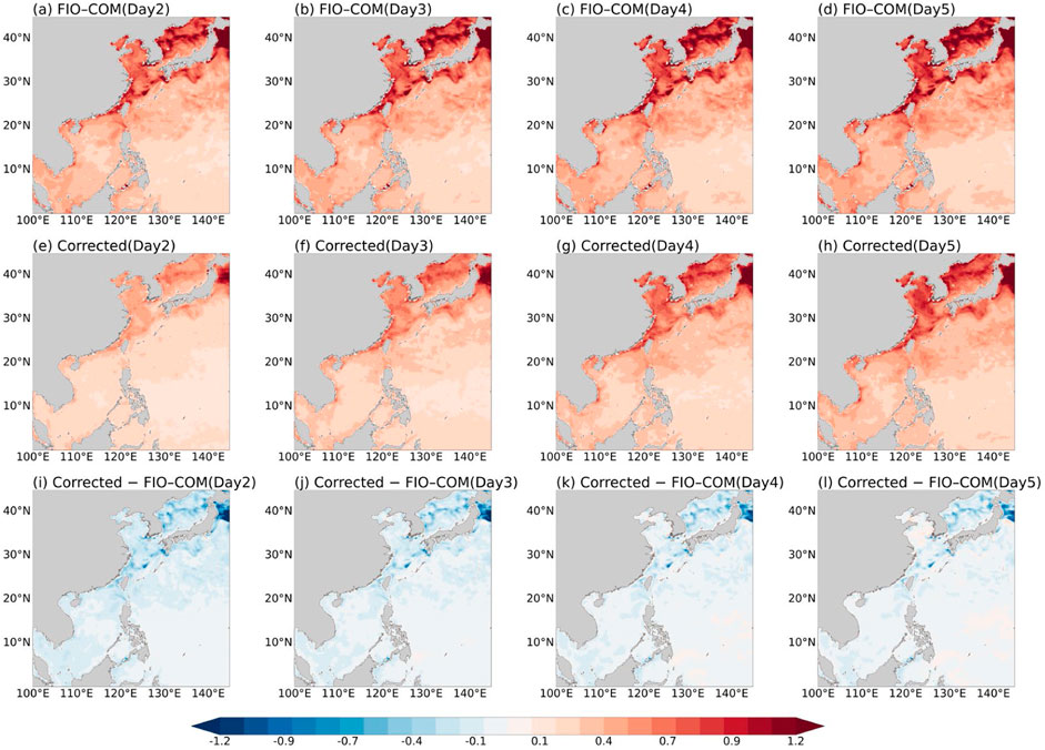
Figure 4. Spatial variability of RMSE (°C) for daily SST forecasts from day 2 to day 5. (a–d) FIO-COM forecasts; (e–h) Post-corrected forecasts; (i–l) RMSE difference between corrected and original forecasts. This figure compares SST forecast accuracy before and after correction.

In the original FIO-COM forecasts (Figures 4a–d), areas of higher uncertainty are evident, particularly in coastal and shelf regions, which exhibit notably higher RMSE values compared to open ocean areas. This spatial variability in forecast accuracy underscores the inherent challenges in modeling regions characterized by complex bathymetry and intricate coastal processes. A clear trend of increasing RMSE values is observed as the forecast horizon extends from day 2 to day 5, reflecting the growing uncertainty associated with longer-range predictions. This progressive degradation of forecast skill aligns with the expected accumulation of errors in numerical models over time.

The Transformer-predicted error variability (Figures 4e–h) demonstrate the model’s capacity to capture and reproduce complex error patterns. These predictions closely mirror the original FIO-COM forecast errors across all forecast days, indicating the model’s success in capturing both large-scale systematic biases and smaller-scale regional variations. The evolution of predicted error patterns from day 2 to day 5 closely follows that of the original forecasts, suggesting that the Transformer model effectively captures not only spatial but also temporal dependencies in the error structure. Notably, the model exhibits comparable skill in predicting error patterns in both open ocean and coastal regions, demonstrating its versatility in handling diverse oceanographic regimes. This capability addresses a key limitation of traditional SST forecasting methods, namely, the challenge of accurately representing processes across different spatial scales.

The RMSE variability of the corrected SST forecasts (Figures 4i–l) provides critical insights into the effectiveness of the Transformer-based correction approach. A marked decrease in RMSE values is observed throughout the domain across all forecast days, indicating the method’s success in addressing both systematic biases and region-specific errors in the original FIO-COM forecasts. The correction appears particularly effective in coastal and shelf regions, where the original forecasts showed the highest errors. This improvement is especially significant given the known challenges in modeling these complex areas. While improvements are evident across all forecast days, the magnitude of error reduction appears to decrease slightly from day 2 to day 5, aligning with the increasing uncertainty inherent in longer-range predictions and suggesting potential areas for future refinement of the method.

This spatial analysis demonstrates the Transformer-based method’s robust performance in improving SST forecast accuracy across diverse oceanographic conditions and forecast horizons. By effectively capturing and correcting complex error patterns, particularly in challenging coastal and dynamically active regions, this approach addresses several key limitations of traditional numerical SST forecasting methods. The results have significant implications for various applications requiring accurate SST predictions, including potential improvements in coupled ocean-atmosphere models and enhanced decision support for marine operations.

A quantitative assessment of the Transformer-based correction method’s effectiveness across different forecast horizons is provided through a comparative analysis of average RMSE between the original FIO-COM and corrected forecasts for day 2 to day 5 (Table 1). This numerical representation demonstrates a substantial reduction in RMSE across all forecast intervals, with the most pronounced improvement observed in the day 2 forecast, exhibiting a 38.8% reduction in RMSE. Such a significant enhancement in short-term forecast accuracy has immediate and far-reaching implications for applications necessitating precise near-term SST predictions, including operational oceanography and short-term marine weather forecasting.

Table 1

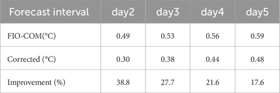
Table 1. Average RMSE (°C) comparison between FIO-COM and corrected forecasts for day 2 to day 5, with post-correction improvement percentages.

While the improvement remains noteworthy across all forecast days, a gradual decrease in the percentage of improvement is observed for longer forecast intervals. Notably, day 5 forecasts still exhibit a 17.6% reduction in RMSE, a considerable improvement given the inherently increased uncertainty associated with longer-range predictions. This persistent enhancement, even at extended forecast horizons, underscores the robustness of the Transformer-based method in capturing and correcting systematic errors across multiple time scales.

Figure 5 presents a comprehensive temporal analysis of median SST forecast errors throughout 2023, demonstrating the substantial improvements achieved through our Transformer-based correction method across different forecast horizons. The original FIO-COM forecasts (Figure 5a) exhibit significant error magnitudes frequently exceeding 0.05°C, with notable temporal variations across the year. After applying our Transformer-based correction (Figure 5b), we observe remarkable enhancements in forecast accuracy across all temporal scales. The corrected forecasts demonstrate significantly reduced error magnitudes, consistently maintaining values within ±0.03°C. Most notably, the correction method effectively mitigates the oscillations present in the original forecasts while preserving essential temporal variability patterns, indicating its robust capability to capture and correct both systematic biases inherent in the numerical model. This improvement is particularly evident in shorter-term predictions, where the corrected forecasts exhibit remarkable stability and consistency throughout the forecasting period.

Figure 5

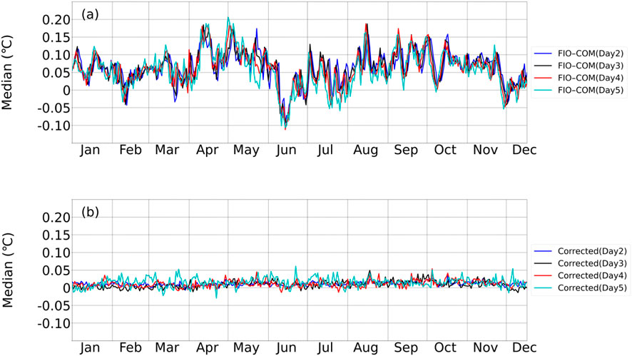
Figure 5. Temporal evolution of median SST forecast errors from the original FIO-COM (a) and after bias correction (b) throughout 2023. Different colored lines indicate varying forecast lead times.

Figure 6 presents a temporal analysis of correlation coefficients between forecasted and observed SST throughout 2023, demonstrating the effectiveness of our Transformer-based correction method. While the original FIO-COM forecasts (Figure 6a) show moderate to strong correlations with notable temporal fluctuations, the Transformer-corrected forecasts (Figure 6b) maintain consistently higher correlations across all temporal scales. This improvement persists across various oceanic conditions and seasonal transitions, though both models exhibit relatively reduced performance during summer months due to increased ocean stratification and variability. The consistent enhancement in forecast accuracy across different temporal scales validates the operational viability of our approach, while also identifying summer predictions as an area for future optimization. These results quantitatively demonstrate the method’s capacity to improve SST forecast reliability for operational oceanographic applications.

Figure 6

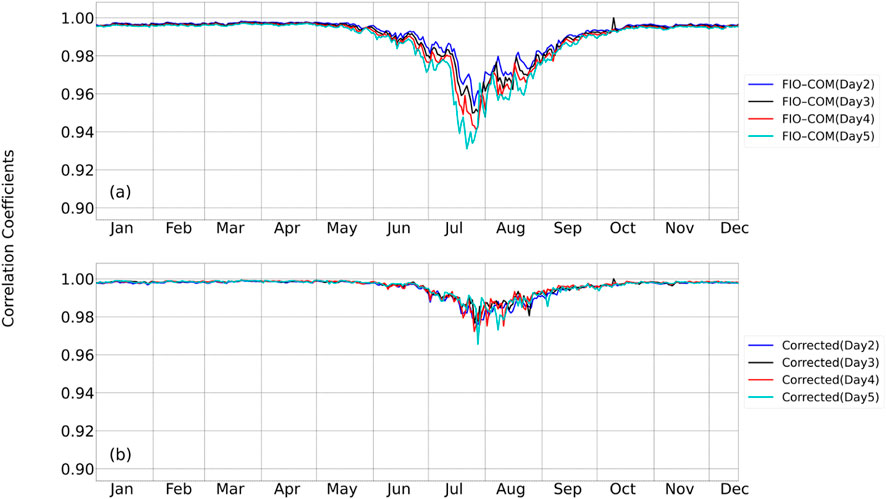
Figure 6. Temporal evolution of correlation coefficients throughout 2023 comparing (a) FIO-COM forecast SST with observational data and (b) bias-corrected SST with observations at various forecast lead times (colored lines). The analysis quantifies the model’s predictive skill before and after bias correction across multiple temporal scales.

3.2 Case evaluation of correction effects

While the RMSE effectively quantifies the overall performance of the FIO-COM numerical forecasting and subsequent transformer-based corrections, it does not provide information about the directional bias of the forecasting error, specifically whether the forecast systematically overestimates or underestimates actual observations. This directional bias, which we refer to as the “phase characteristic” of the forecasting error, is crucial for understanding the nature of forecast inaccuracies. To gain a more comprehensive understanding of the forecasting effectiveness, additional error statistical metrics and further analysis of error distributions are necessary to capture these directional tendencies in forecast errors.

To provide a more detailed insight into the performance of our correction method, an in-depth case study was conducted, focusing on a forecast initiated at 1200 UTC 4 January 2023. This specific case was chosen as it demonstrates a clear and pronounced correction effect, allowing for a more distinct visualization of the method’s capabilities. While this case exhibits better-than-average performance, it serves to highlight the potential of our approach under favorable conditions. This case study examines the spatial and temporal characteristics of the correction effects at a higher resolution, offering insights into the method’s performance under specific oceanic conditions. A comprehensive visualization of the spatial error variability for this case study (Figure 7) illustrates how the Transformer-based method performs in correcting SST forecast errors across different regions and forecast horizons.

Figure 7a illustrates the spatial distribution of FIO-COM model forecast errors at day 1, which serves as input for the transformer model to predict forecast errors from day 2 to day 5. The original FIO-COM forecast errors (Figures 7b–e) exhibit intricate spatial patterns of over- and under-prediction across the study domain, particularly pronounced in coastal areas, near strong currents, and in regions of known mesoscale activity. A clear trend of increasing error magnitude is observed as the forecast horizon extends from day 2 to day 5, consistent with the expected degradation of forecast skill over time. Certain regions consistently show larger errors across all forecast days, likely indicating areas where the original model struggles to capture local dynamics accurately.

Figure 7

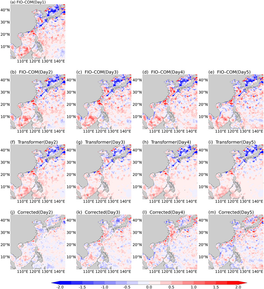
Figure 7. Spatial error variability (Units: °C) in daily SST forecasts initiated at 1200 UTC 4 January 2023. (a–e) Original FIO-COM forecast errors from day 1 to day 5; (f–i) Transformer-predicted error patterns; (j–m) Corrected SST errors after Transformer adjustment.

The Transformer-predicted error patterns (Figures 7f–i) demonstrate the model’s remarkable capability to capture the overall spatial structure of forecast errors. The high similarity between these predicted patterns and the original FIO-COM errors attests to the model’s feature extraction and attention mechanisms. The predicted error patterns show sensitivity to both large-scale systematic biases and smaller-scale regional variations, indicating the model’s ability to correct errors across different spatial scales. Furthermore, the logical evolution of predicted error patterns from day 2 to day 5 suggests that the model captures both spatial and temporal dependencies in the error structure.

The residual errors after applying the Transformer-based correction (Figures 7j–m) provide critical insights into the method’s effectiveness. A marked decrease in error magnitude is observed across the entire domain, with notable improvements in areas that initially had the largest errors. The correction addresses large-scale biases while retaining small-scale variability. Although greatly reduced, some error patterns persist in the corrected forecasts, particularly at longer lead times, likely representing the limits of predictability or indicating areas for potential further improvement. Notably, the correction appears particularly effective in coastal and shelf regions, addressing a key challenge in SST forecasting. It's worth noting that differences between the model’s coastline representation and the observed coastline, due to model resolution limitations, can generate systematic errors that our bias correction mechanism aims to identify and address.

This detailed spatial analysis demonstrates the Transformer-based method’s ability to provide targeted, spatially-aware corrections to SST forecasts. The model’s success in capturing and correcting complex error patterns across different regions and forecast horizons addresses many challenges associated with traditional numerical SST forecasting methods, particularly in areas of complex ocean dynamics. These results underscore the potential of the Transformer-based approach to enhance the accuracy and reliability of SST forecasts across diverse oceanographic conditions.

An interesting pattern emerges from the analysis of FIO-COM forecast errors from day 1 to day 5 (Figures 7a–e), revealing remarkable spatial similarity in error distribution patterns. This observation led to an investigation of whether the day 1 forecast errors could serve as a proxy for error correction in subsequent days. We explored this hypothesis by implementing two correction strategies: (1) directly applying day 1 errors to correct forecasts from day 2 to day 5, and (2) using our transformer model to retrieve specific forecast errors for each day.

Table 2 presents a quantitative comparison of RMSE (°C) among three approaches: the original FIO-COM forecasts, forecasts corrected using day 1 errors, and forecasts corrected using retrieved errors. The original FIO-COM forecasts show a gradual increase in RMSE from 0.63°C at day 2°C to 0.67°C at day 5, reflecting the expected degradation in forecast accuracy over time. Both correction methods demonstrate substantial improvement in forecast accuracy, with the transformer-based error retrieval method consistently outperforming the direct day 1 error correction approach. Specifically, while the day 1 error correction reduces RMSE to 0.32°C at day 2°C and 0.50°C at day 5, the transformer model achieves even lower RMSE values of 0.28°C and 0.46°C for the same forecast days, respectively. The superior performance of the transformer-based approach demonstrates its capability to capture the temporal evolution of forecast errors more accurately than the simple persistence assumption underlying the day 1 error correction method. This advantage becomes particularly evident at longer forecast horizons, where the transformer model maintains better forecast skill through its ability to learn and adapt to the dynamic nature of error patterns across different forecast lengths.

Table 2

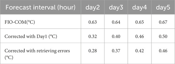
Table 2. RMSE (°C) comparison of daily SST forecasts among the original FIO-COM, day1 error correction, and retrieved-error correction methods for the case initiated at 1200 UTC 4 January 2023.

The error variability comparison between FIO-COM forecasts and Transformer-predicted errors (Figure 8) provides a comprehensive evaluation of the correction method’s effectiveness across different forecast horizons. The scatter plots reveal that the Transformer-based method is particularly adept at correcting larger FIO-COM errors, as evidenced by the tighter clustering of points along the diagonal in the first and third quadrants for larger error magnitudes. This pattern is consistent across all forecast days (day 2 to day 5), highlighting the method’s robustness in addressing significant forecast discrepancies. Conversely, for smaller FIO-COM errors, the correction effects are less pronounced, as indicated by the wider scatter of points near the origin. However, this reduced effectiveness for minor errors is less critical from an operational perspective, as these errors are already within an acceptable range. Notably, the gradual increase in point dispersion from day 2 to day 5 aligns with the decreasing percentage improvement in RMSE observed in Table 1, reflecting the growing challenges in error correction over extended forecast periods. Despite this trend, the predominance of points in the first and third quadrants across all forecast days demonstrates the model’s consistent ability to provide corrections, even for longer-range forecasts. These findings underscore the Transformer-based method’s potential to enhance SST forecast accuracy, particularly in scenarios with larger initial errors.

Figure 8

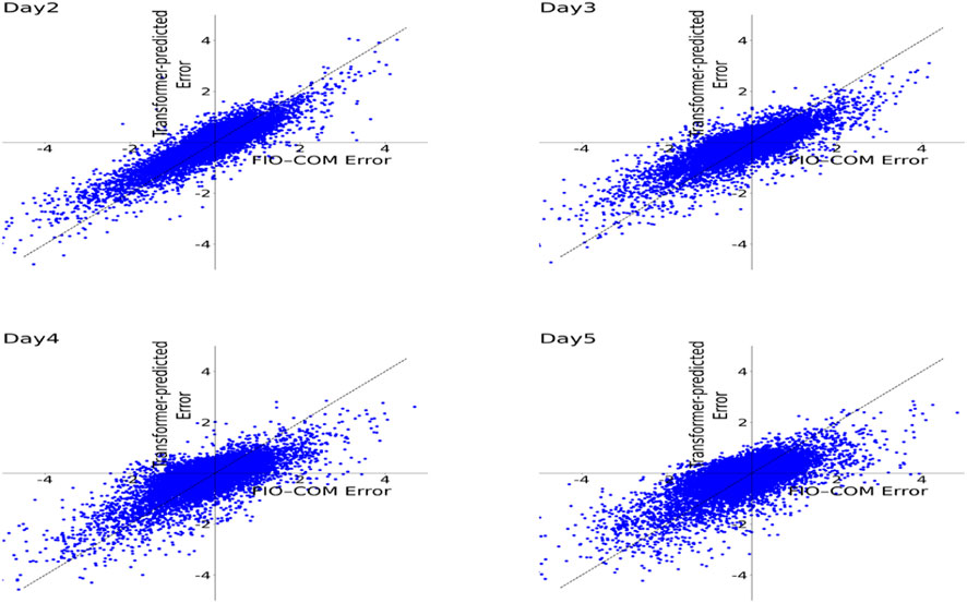
Figure 8. Error variability comparison (°C) between FIO-COM forecasts and Transformer-predicted errors for the case initiated at 1200 UTC 4 January 2023. Variabilities for day 2 to day 5 forecasts.

To provide a more rigorous quantitative assessment of the correction effectiveness beyond visual scatter plot analysis, we conducted a detailed statistical evaluation examining the proportion of successfully corrected grid points across different error magnitude ranges. Table 3 provides a granular analysis of the correction effectiveness, categorizing the results based on the magnitude of FIO-COM forecasting errors. For errors exceeding ±1°C, the correction method achieved remarkable effectiveness, with success rates of 98.9% and 97.8% for negative and positive errors respectively at day 2 forecasts. This high correction rate persisted even at longer forecast horizons, maintaining above 89% effectiveness through day 5. For moderate errors (−1°C ≤ Error ≤1°C), the method demonstrated solid performance with correction rates of 78.9% at day 2, gradually decreasing to 69.6% by day 5. These results quantitatively confirm the visual patterns observed in the scatter plots and underscore the Transformer-based method’s particular strength in addressing significant forecast deviations while maintaining effectiveness for smaller errors, further validating its potential for operational implementation in SST forecasting systems.

Table 3

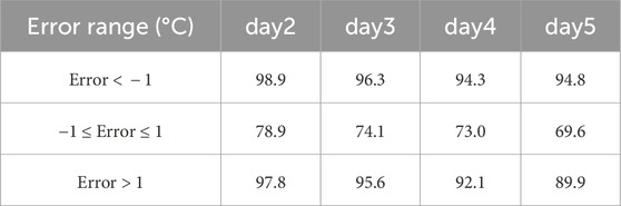
Table 3. Percentage of effectively corrected grid points in FIO-COM SST forecasts initiated at 1200 UTC 4 January 2023, for forecast horizons from day 2 to day 3.

4 Conclusion

This study demonstrates the effectiveness of a Transformer-based method for correcting daily SST numerical forecasting products through comprehensive quantitative analysis. Our method achieved significant and consistent RMSE reductions compared to the original FIO-COM forecasts, with improvements ranging from 38.8% for day 2 forecasts to 17.6% for day 5 forecasts. Spatial analysis revealed robust performance across the study region, with particularly strong improvements in coastal and shelf areas where the original model exhibited higher RMSE values. The temporal analysis further validated the method’s reliability, with correlation coefficients between forecasted and observed SST showing sustained improvement across all forecast horizons. Notably, for errors exceeding ±1°C, the method achieved correction rates of 98.9% and 97.8% for negative and positive errors respectively at day 2 forecasts, maintaining above 89% effectiveness through day 5.

The demonstrated improvements have significant implications for operational oceanography and marine forecasting applications. While the correction effectiveness gradually decreases for longer forecast intervals, as evidenced by the reduction in improvement from 38.8% to 17.6% between day 2 and day 5, the method maintains substantial benefits throughout all analyzed periods. These enhancements in forecast accuracy directly address key limitations in current SST forecasting capabilities, particularly in operational settings where rapid and accurate predictions are essential for decision-making processes. The method’s consistent performance across varying conditions supports its potential integration into operational forecasting systems.

The practical applications of these improvements extend to various sectors dependent on accurate SST predictions. Enhanced forecast accuracy could significantly benefit fisheries management, maritime operations, and resource management activities. The method’s ability to provide more reliable SST forecasts, particularly in challenging coastal regions, offers potential for improving operational decision-making processes across multiple maritime sectors. While this approach does not directly enhance our understanding of physical processes, its demonstrated capability to correct systematic errors in existing models makes it a valuable tool for improving operational SST forecasting.

Future research directions should focus on several key areas to further advance this methodology. Priority areas include extending the approach to other oceanographic variables and regions, investigating performance enhancements for extended forecast periods through additional parameter incorporation, and comparing the method’s effectiveness with other machine learning approaches such as CNNs and PCA. Additionally, evaluating the method’s integration into operational systems warrants careful investigation. These findings contribute to the growing evidence supporting the integration of machine learning techniques with traditional numerical modeling approaches in oceanographic forecasting, while maintaining emphasis on quantifiable improvements and practical applications.

Data availability statement

The original contributions presented in the study are publicly available. This data can be found here: https://drive.google.com/file/d/1X8z-_1N4pU0YM_XMATPWHaqxc38ENmds/view.

Author contributions

GZ: Conceptualization, Methodology, Software, Writing–original draft. XK: Conceptualization, Methodology, Writing–original draft, Writing–review and editing. YL: Formal Analysis, Writing–review and editing. QW: Validation, Visualization, Writing–review and editing. HS: Validation, Writing–review and editing. XY: Data curation, Writing–review and editing.

Funding

The author(s) declare that financial support was received for the research and/or publication of this article. Scientific Research Startup Funding for High-Level Talent Introduction at Civil Aviation Flight University of China (Grant No. XYKY2024064). This research was supported financially by Laoshan Laboratory (LSKJ202202103).

Acknowledgments

We acknowledge Lu Zhou for the foundational 3DGeoformer code (https://github.com/zhoulu327/Code_of_3DGeoformer/commits/v1.0), which provided a critical starting point for our research. Building upon this framework, we have adapted and refined the original 3D-Geoformer architecture to address the specific challenges of 2D SST error prediction.

Conflict of interest

The authors declare that the research was conducted in the absence of any commercial or financial relationships that could be construed as a potential conflict of interest.

Generative AI statement

The author(s) declare that no Generative AI was used in the creation of this manuscript.

Publisher’s note

All claims expressed in this article are solely those of the authors and do not necessarily represent those of their affiliated organizations, or those of the publisher, the editors and the reviewers. Any product that may be evaluated in this article, or claim that may be made by its manufacturer, is not guaranteed or endorsed by the publisher.

References

Agabin, A., Prochaska, J. X., Cornillon, P. C., and Buckingham, C. E. (2024). Mitigating masked pixels in a climate-critical ocean dataset. Remote Sens. 16, 2439. doi:10.3390/rs16132439

CrossRef Full Text | Google Scholar

Alerskans, E., Nyborg, J., Birk, M., and Kaas, E. (2022). A transformer neural network for predicting near-surface temperature. Meteorol. Appl. 29, e2098. doi:10.1002/met.2098

CrossRef Full Text | Google Scholar

Ali, A., Fathalla, A., Salah, A., Bekhit, M., and Eldesouky, E. (2021). Marine data prediction: an evaluation of machine learning, deep learning, and statistical predictive models. Comput. Intell. Neurosci. 2021, 8551167. doi:10.1155/2021/8551167

PubMed Abstract | CrossRef Full Text | Google Scholar

Barton, N., Metzger, E. J., Reynolds, C. A., Ruston, B., Rowley, C., Smedstad, O. M., et al. (2021). The Navy's Earth System Prediction Capability: a new global coupled atmosphere-ocean-sea ice prediction system designed for daily to subseasonal forecasting. Earth Space Sci. 8, e2020EA001199. doi:10.1029/2020ea001199

CrossRef Full Text | Google Scholar

Belyaev, K., Kuleshov, A., Smirnov, I., and Tanajura, C. A. S. (2021). Generalized kalman filter and ensemble optimal interpolation, their comparison and application to the hybrid coordinate ocean model. Mathematics 9, 2371. doi:10.3390/math9192371

CrossRef Full Text | Google Scholar

Bennis, A. C., Furgerot, L., and Du, B. P. B. (2020). Numerical modelling of three-dimensional wave-current interactions in complex environment: application to Alderney Race. Appl. Ocean. Res. 95, 102021. doi:10.1016/j.apor.2019.102021

CrossRef Full Text | Google Scholar

Busecke, J., Balwada, D., and Martin, P. (2024). The overlooked sub-grid air-sea flux in climate models.

Google Scholar

Chassignet, E. P., Hurlburt, H. E., Metzger, E. J., Smedstad, O., Cummings, J., Halliwell, G., et al. (2009). US GODAE: global ocean prediction with the HYbrid Coordinate Ocean Model (HYCOM). Oceanography 22, 64–75. doi:10.5670/oceanog.2009.39

CrossRef Full Text | Google Scholar

Dai, H., He, Z., Wei, G., Lei, F., Zhang, X., Zhang, W., et al. (2024). Long-term prediction of Sea Surface temperature by temporal embedding transformer with attention distilling and partial stacked connection. IEEE J. Sel. Top. Appl. Earth Obs. Remote Sens. 17, 4280–4293. doi:10.1109/jstars.2024.3357191

CrossRef Full Text | Google Scholar

de, L. C., Vic, C., Madec, G., Roquet, F., Waterhouse, A. F., Whalen, C. B., et al. (2020). A parameterization of local and remote tidal mixing. J. Adv. Model. Earth Syst. 12, e2020MS002065. doi:10.1029/2020ms002065

CrossRef Full Text | Google Scholar

de, R. P., Browne, P., and de, B. E. (2022). Coupled data assimilation at ECMWF: current status, challenges and future developments. Q. J. R. Meteorol. Soc. 148, 2672–2702. doi:10.1002/qj.4330

CrossRef Full Text | Google Scholar

Deser, C., Alexander, M. A., Xie, S. P., and Phillips, A. S. (2010). Sea surface temperature variability: patterns and mechanisms. Annu. Rev. Mar. Sci. 2, 115–143. doi:10.1146/annurev-marine-120408-151453

PubMed Abstract | CrossRef Full Text | Google Scholar

Elafi, I., Zrira, N., Kamal-Idrissi, A., Khan, H. A., and Ettouhami, A. (2024). STA-SST: spatio-temporal time series prediction of Moroccan Sea surface temperature. J. Sea Res. 200, 102515. doi:10.1016/j.seares.2024.102515

CrossRef Full Text | Google Scholar

Fei, T., Huang, B., Wang, X., Zhu, J., Chen, Y., Wang, H., et al. (2022). A hybrid deep learning model for the bias correction of sst numerical forecast products using satellite data. Remote Sens. 14, 1339. doi:10.3390/rs14061339

CrossRef Full Text | Google Scholar

Ferrari, R., McWilliams, J. C., Canuto, V. M., and Dubovikov, M. (2008). Parameterization of eddy fluxes near oceanic boundaries. J. Clim. 21, 2770–2789. doi:10.1175/2007jcli1510.1

CrossRef Full Text | Google Scholar

Fyfe, J. C., Kharin, V. V., Santer, B. D., Cole, J. N. S., and Gillett, N. P. (2021). Significant impact of forcing uncertainty in a large ensemble of climate model simulations. Proc. Nat. Acad. Sci. 118, 2016549118. doi:10.1073/pnas.2016549118

PubMed Abstract | CrossRef Full Text | Google Scholar

Goh, E., Yepremyan, A., Wang, J., and Wilson, B. (2024). MAESSTRO: masked autoencoders for Sea Surface temperature reconstruction under occlusion. Ocean. Sci. 20, 1309–1323. doi:10.5194/os-20-1309-2024

CrossRef Full Text | Google Scholar

Kang, X., Song, H., Zhang, Z., Yin, X., and Gu, J. (2024). A transformer-based method for correcting significant wave height numerical forecasting errors. Front. Mar. Sci. 11, 1374902. doi:10.3389/fmars.2024.1374902

CrossRef Full Text | Google Scholar

Kessler, A., Goris, N., and Lauvset, S. K. (2022). Observation-based Sea surface temperature trends in Atlantic large marine ecosystems. Prog. Oceanogr. 208, 102902. doi:10.1016/j.pocean.2022.102902

CrossRef Full Text | Google Scholar

Manda, A., Hirose, N., and Yanagi, T. (2005). Feasible method for the assimilation of satellite-derived SST with an ocean circulation model. J. Atmos. Ocean. Technol. 22, 746–756. doi:10.1175/jtech1744.1

CrossRef Full Text | Google Scholar

Meng, Z., and Hakim, G. J. (2024). Reconstructing the tropical Pacific upper ocean using online data assimilation with a deep learning model. J. Adv. Model. Earth Syst. 16 (11), e2024MS004422. doi:10.1029/2024ms004422

PubMed Abstract | CrossRef Full Text | Google Scholar

Miller, A. J., Collins, M., Gualdi, S., Jensen, T. G., Misra, V., Pezzi, L. P., et al. (2017). Coupled ocean–atmosphere modeling and predictions. J. Mar. Res. 75, 361–402. doi:10.1357/002224017821836770

CrossRef Full Text | Google Scholar

O’dea, E. J., Arnold, A. K., Edwards, K. P., Furner, R., Hyder, P., Martin, M. J., et al. (2012). An operational ocean forecast system incorporating NEMO and SST data assimilation for the tidally driven European North-West shelf. J. Oper. Oceanogr. 5, 3–17. doi:10.1080/1755876x.2012.11020128

CrossRef Full Text | Google Scholar

Patil, K., and Deo, M. C. (2017). Prediction of daily sea surface temperature using efficient neural networks. Ocean. Dyn. 67, 357–368. doi:10.1007/s10236-017-1032-9

CrossRef Full Text | Google Scholar

Planque, B., Fox, C. J., Saunders, M. A., and Rockett, P. (2003). On the prediction of short term changes in the recruitment of North Sea cod (Gadus morhua) using statistical temperature forecasts. Sci. Mar. 67, 211–218. doi:10.3989/scimar.2003.67s1211

CrossRef Full Text | Google Scholar

Qiao, F., Wang, G., Khokiattiwong, S., Akhir, M. F., Zhu, W., and Xiao, B. (2019). China published ocean forecasting system for the 21st-Century Maritime Silk Road on December 10, 2018. Acta Oceanol. Sin. 38, 1–3. doi:10.1007/s13131-019-1365-y

CrossRef Full Text | Google Scholar

Sarkar, P. P., Janardhan, P., and Roy, P. (2020). Prediction of sea surface temperatures using deep learning neural networks. SN Appl. Sci. 2, 1458. doi:10.1007/s42452-020-03239-3

CrossRef Full Text | Google Scholar

Schade, L. R. (2000). Tropical cyclone intensity and Sea Surface temperature. J. Atmos. Sci. 57, 3122–3130. doi:10.1175/1520-0469(2000)057<3122:tciass>2.0.co;2

CrossRef Full Text | Google Scholar

Shao, Q., Li, W., Han, G., Hou, G., Liu, S., Gong, Y., et al. (2021). A deep learning model for forecasting sea surface height anomalies and temperatures in the South China Sea. J. Geophys. Res-Oceans 126, e2021JC017515. doi:10.1029/2021jc017515

CrossRef Full Text | Google Scholar

Stanev, E. V., Ricker, M., Grayek, S., Jacob, B., Haid, V., and Staneva, J. (2020). Numerical eddy-resolving modeling of the ocean: mesoscale and sub-mesoscale examples. Phys. Oceanogr. 27, 631–658. doi:10.22449/1573-160x-2020-6-631-658

CrossRef Full Text | Google Scholar

Vaswani, A. (2017). Attention is all you need. Adv. Neural Inf. Process. Syst. doi:10.48550/arXiv.1706.03762

CrossRef Full Text | Google Scholar

Wei, M., Jacobs, G., Rowley, C., Barron, C. N., Hogan, P., Spence, P., et al. (2016). The performance of the US Navy's RELO ensemble, NCOM, HYCOM during the period of GLAD at-sea experiment in the Gulf of Mexico. Deep-Sea Res. Part II-Top. Stud. Oceanogr. 129, 374–393. doi:10.1016/j.dsr2.2013.09.002

CrossRef Full Text | Google Scholar

Xie, B., Qi, J., Yang, S., Sun, G., Feng, Z., Yin, B., et al. (2024). Sea surface temperature and marine heat wave predictions in the south China Sea: a 3D U-net deep learning model integrating multi-source data. Atmosphere 15, 86. doi:10.3390/atmos15010086

CrossRef Full Text | Google Scholar

Yu, X., Shi, S., Xu, L., Liu, Y., Miao, Q., and Sun, M. (2020). A novel method for sea surface temperature prediction based on deep learning. Math. Probl. Eng. 2020, 1–9. doi:10.1155/2020/6387173

CrossRef Full Text | Google Scholar

Zhou, L., and Zhang, R. H. (2023). A self-attention–based neural network for three-dimensional multivariate modeling and its skillful ENSO predictions. Sci. Adv. 9, eadf2827. doi:10.1126/sciadv.adf2827

PubMed Abstract | CrossRef Full Text | Google Scholar

Zhu, Y., and Zhang, R. H. (2019). A modified vertical mixing parameterization for its improved ocean and coupled simulations in the tropical Pacific. J. Phys. Oceanogr. 49, 21–37. doi:10.1175/jpo-d-18-0100.1

CrossRef Full Text | Google Scholar

Zou, R., Wei, L., and Guan, L. (2023). Super resolution of satellite-derived Sea Surface temperature using a transformer-based model. Remote Sens. 15, 5376. doi:10.3390/rs15225376

CrossRef Full Text | Google Scholar

Zrira, N., Kamal-Idrissi, A., Farssi, R., and Khan, H. A. (2024). Time series prediction of sea surface temperature based on BiLSTM model with attention mechanism. J. Sea Res. 198, 102472. doi:10.1016/j.seares.2024.102472

CrossRef Full Text | Google Scholar