Improvement of rock surface roughness accuracy by combining object space resolution error and 3D point cloud features

To enhance the accuracy of joint roughness coefficient (JRC) estimation in photogrammetry, this study employed a fixed-camera shooting strategy guided by a Structure-from-Motion-based shooting parameter selection algorithm to reconstruct 3D models of rock samples at 16 different shooting distances. The analysis at profile intervals of 0.25 mm, 0.5 mm, and 1 mm revealed a strong correlation between JRC accuracy and three parameters: object space resolution error, spatial distance between point cloud points, and spatial errors of checkpoints on the orientation board. Using these three parameters as input variables and JRC error as the output variable, five machine learning algorithms—Support Vector Regression, Gaussian Process Regression, Multilayer Perceptron, XGBoost, and CatBoost—were employed to predict JRC errors across different shooting distances. The Multilayer Perceptron model performed best at profile intervals of 0.25 mm and 0.5 mm, while XGBoost was optimal at the 1 mm interval. Under the predictions of these models, JRC accuracy improved by an average of 84.7% across the three intervals. Finally, the applicability and limitations of the proposed method were further discussed.

1 Introduction

Accurately estimating the joint roughness coefficient (JRC) is crucial for evaluating the stability of rock masses in engineering projects like slopes, tunnels, and underground caverns (ISRM, 1978). The JRC, which plays a key role in geological sketching for rock engineering, provides insight into the shear strength of rock joints (Patton, 1966; Barton and Choubey, 1977). In recent years, non-contact measurement methods for rock joint characterization, represented by laser scanning and photogrammetry techniques, have been extensively studied and applied by numerous researchers (Fardin et al., 2001; Ge et al., 2012; Cignetti et al., 2019; Francioni et al., 2019). These advanced optical and computational technologies enable the rapid acquisition of high-resolution 3D models of rock joints, which can be used to quantify joint roughness parameters and further estimate the shear strength of rock joints (Tse and Cruden, 1979; Grasselli and Egger, 2003; Ge et al., 2014; Lin et al., 2021; Ge et al., 2022; Lin et al., 2024; Yong et al., 2024).

With the rapid development of computer vision, optical measurement, and sensor technologies, photogrammetry, known for its low cost, portability, and short data processing time, has gained widespread popularity and usage in obtaining the JRC (Battulwar et al., 2021; Ge et al., 2022; Xia et al., 2022; Ling et al., 2022; Paixão et al., 2022). García-Luna et al. (2021) used a camera and tripod to collect images of slope rock masses, analyzing the impact of shooting distance, focal length, and the number of images on roughness. Paixão et al. (2022) provided a detailed description of the application process of the Structure-from-Motion (SfM) photogrammetry method in estimating the surface roughness of small-scale rock samples, exploring the effects of shooting angles, angular intervals, and data processing software on JRC accuracy. Ge et al. (2022) employed a similar data collection strategy to investigate the performance of smartphones in estimating JRC and compared the results with those obtained using digital cameras. Due to smartphones utilizing CMOS sensors, the resulting JRC accuracy was lower. In the same year, An et al. (2022) employed a similar convergence strategy to estimate the roughness of small-scale rock samples and proposed the “moving smartphone capture” method, which uses only a smartphone. When comparing the results with those obtained using data collection methods involving fixed devices such as tripods and turntables, the latter demonstrated higher JRC accuracy.

The detailed examination of photogrammetry techniques utilizing SfM technology reveals a shift in JRC assessment towards greater cost-efficiency and ease of use. However, it must be acknowledged that in practical applications, regardless of the hardware used or the implementation of fixed settings, JRC estimates will inevitably deviate to some extent from actual values. Moreover, parameters such as camera resolution and shooting position cannot always be optimally configured. Although numerous studies have investigated the effects of factors like equipment resolution and shooting configurations on errors in roughness parameter estimation (García-Luna et al., 2021; An et al., 2022; Ge et al., 2022; Yang et al., 2024), there is still a lack of research focused on innovative methods to improve JRC accuracy in photogrammetry. Against this backdrop, machine learning technology emerges as a powerful tool for addressing complex nonlinear problems with multiple intertwined parameters, offering new insights and approaches for optimizing JRC accuracy in photogrammetry. The introduction of this cutting-edge technology not only breathes new life into traditional photogrammetry methods but also holds the potential for significant improvements in JRC estimation accuracy. By leveraging machine learning algorithms for in-depth analysis of large datasets, it is possible to uncover more potential factors affecting estimation accuracy and design more precise and efficient estimation models.

This study aims to improve the accuracy of photogrammetric JRC estimation using machine learning algorithms. Initially, rock sample point cloud models were collected through a combination of a camera parameter selection algorithm and a tripod-based data acquisition strategy. The study then investigated the effects of object space resolution error, spatial distance, and spatial error on JRC estimation accuracy. Finally, five machine learning algorithms were employed to predict JRC errors at different shooting distances, resulting in the development of a photogrammetric JRC accuracy optimization model based on the tripod strategy.

2 Methodology

2.1 Point cloud extracted from SfM-based photogrammetric data

The SfM-based photogrammetry technique has become a standard in rock engineering applications (Hartley and Sturm, 1997; Kong et al., 2021). As depicted in Figure 1A, the process starts by identifying feature points ($P_{mj}$) from two initial images and matching them with corresponding target points ($P_j$). This matching process helps estimate the initial camera positions ($O_1$, $O_2$). These correspondences are then extended across additional images to refine the camera pose ($O_m$) estimates for each image. Using this information, a sparse 3D model of the scene is constructed. Subsequently, depth maps, which represent the depth values of all pixels, are generated and combined into a single, consistent depth map (see Figure 1B). Finally, a dense point cloud is produced from the merged depth map, as illustrated in Figure 1C.

Figure 1

Figure 1. Overview of SfM-based photogrammetry in rock data acquisition. (A) The principle of SfM-based photogrammetry. (B) A rock depth map. (C) A 3D rock model.

2.2 Specimen preparation and experimental setup

Figure 2 illustrates the use of the underside of an artificially split sandstone sample as the test object. This sample, which has a slightly uneven surface, measures 100 × 100 × 50 mm. It is placed within an orientation plate (OP) equipped with four ground control points (GCPs) spaced 160 mm apart. The OP is utilized to orient and scale the point cloud of the rock sample. Additionally, the OP contains twelve checkpoints (CPs). The discrepancy between the point cloud coordinates of these checkpoints and their actual coordinates provides a partial measure of the point cloud reconstruction quality (ASPRS, 2015; Cultural Heritage Imaging, 2015). According to Agisoft Metashape (2022) guidelines, the checkpoint size is set to five times the ground sampling distance (GSD), which is determined by the image pixel count (Yang et al., 2024).

Figure 2

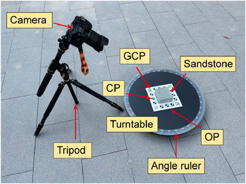
Figure 2. JRC estimation experiment for small-scale rock sample.

Images of the target rock samples were captured using a Canon EOS 90D digital single-lens reflex (DSLR) camera. The camera uses a high-resolution CCD sensor with a sensor size of 22.3 × 14.8 mm and a pixel capacity of 6,960 × 4,640 pixels. The lens used is EF-S 18–135 mm f/3.5–5.6 IS USM. To precisely control the relative position and angle between the rock samples and the camera, a turntable and tripod were utilized as support and adjustment tools. Additionally, a precision angle ruler was employed to accurately adjust the rotation angle of the rocks, allowing images to be captured at each angular interval. Natural lighting was used to accurately reflect the rock’s morphology under authentic environmental conditions. As shown in Figure 2, a field rock specimen roughness measurement setup was established.

2.3 Data acquisition

The fixed camera capture (FCC) method offers a cost-effective way to capture rock images, ensuring high image overlap and providing excellent stability and ease of use (Ge et al., 2022). The shooting parameter selection algorithm (SPSA), introduced by Yang et al. (2024), generates tailored shooting parameters based on the specific camera and rock dimensions. In this study, FCC is utilized in conjunction with SPSA, following the principles of SfM.

To begin with, the specific dimensions of the target rock, the GSD, and the key parameters of the imaging equipment were all entered into the SPSA, as detailed in Table 1. In this study, the camera’s shooting angle and positional interval adhered to the professional recommendations of Ge et al. (2022), being set at 30° and 15° respectively. This configuration facilitated the capture of 24 high-resolution images to ensure a high degree of image overlap. Furthermore, in accordance with the guidelines provided by Edmund Optics (2023), one-third of the GSD was set as the threshold for spatial resolution, intended to allow a reasonable tolerance for uncertainty in the accuracy of spatial points during the 3D reconstruction process, thereby enhancing the reliability of the results. Subsequently, based on SPSA calculations, with a GSD set at 1, the camera’s shooting layout at various positions is illustrated in Figure 3. These positions were sampled at 100 mm intervals. It is noteworthy that the positions depicted in Figure 3 not only indicate spatial locations but also visually represent the dynamic variations in objective space resolution error (OSRE) through changes in size and color.

Table 1

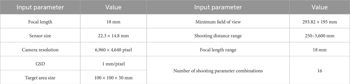
Table 1. Application of shooting parameter selection algorithm.

Figure 3

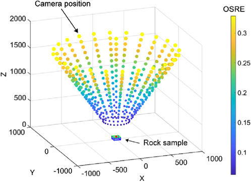
Figure 3. Results of SPSA generation based on convergence strategy.

2.4 Data processing and JRC estimation

Agisoft Metashape (2022) was chosen for the three-dimensional reconstruction of the rock surface, as it aligns with the SfM principle. The reconstruction parameters were configured with the highest alignment accuracy, and the depth maps and point clouds were generated with exceptional precision. For the GCPs, the software automatically identified these points within the point cloud using the imported real-world coordinates, facilitating the overall rotation and scaling of the point cloud. Following this, CloudCompare (2023) was used to segment and extract the rock surface point cloud, standardizing its dimensions and enabling the analysis of JRC variations across different shooting distances.

Object space resolution is a variable that reflects the density of 3D point clouds, determined by shooting parameters and pixel size. According to the study by Yang et al. (2024), a strong correlation exists between the object space resolution error (OSRE) and the JRC error. The equation for calculating this value is as follows:

$Erro{r}_{\text{OSR}}=\frac{hf}{Z-f}(1)$

where $h$ is the pixel size, $f$ is the camera focal length, $Z$ is the shooting distance, and $Erro{r}_{\text{OSR}}$ is the calculated value of OSRE. This value can be calculated solely using the shooting parameters.

In studies evaluating joint roughness, the spatial distance between points in the point cloud reflects the accuracy of the roughness to some extent (Paixão et al., 2022; Ge et al., 2022). This value is defined as the ratio of the area of the selected rock surface point cloud to the number of points, and it can be calculated using statistics from post-processing software.

According to the positional accuracy standards for digital geospatial data provided by the American Society for Photogrammetry and Remote Sensing (ASPRS), researchers can evaluate point cloud accuracy using the spatial errors of check points (ASPRS, 2015). The spatial error between the point cloud coordinates and the true coordinates of the twelve checkpoints, used as a parameter to reflect JRC accuracy in this study, is represented by the average root mean quare error (RMSE) calculated manually, as shown in Equation 2:

$RMSE=\sqrt{\frac{1}{n}{\displaystyle \sum _{i=1}^n}{\left(x_{ia}-x_{ib}\right)}^2+\frac{1}{n}{\displaystyle \sum _{i=1}^n}{\left(y_{ia}-y_{ib}\right)}^2+\frac{1}{n}{\displaystyle \sum _{i=1}^n}{\left(z_{ia}-z_{ib}\right)}^2}(2)$

where $x_{ia}$, $y_{ia}$, $z_{ia}$ represent the coordinates of the center point of CPs in the point cloud, while $x_{ib}$, $y_{ib}$, $z_{ib}$ represent the true coordinates of CPs in the OP. $n$ denotes the number of CPs. $RMSE$ represents the spatial error (ASPRS, 2015).

In rock engineering, the JRC is essential for classifying rock mass quality and assessing stability (Barton and Choubey, 1977; ISRM, 1978). When estimating JRC from point cloud coordinates, the accuracy is significantly affected by the choice of profile intervals (PI) (Tse and Cruden, 1979). Following the method outlined by Yu and Vayssade (1991), JRC values for profile intervals of 0.25 mm, 0.5 mm, and 1 mm were calculated using Equations 3, 4 and are shown in Figure 4. The JRC for each profile ($JR{C}_{2D}$) is determined using $Z_2$:

$Z_2=\sqrt{\frac{1}{L}{\displaystyle \sum _{i=1}^{N-1}}\frac{\left(z_{i+1}-z_i\right)}{x_{i+1}-x_i}}(3)$

$\left\{\begin{array}{l}JR{C}_{2D}=60.32Z_2-4.51\left(\text{for\hspace{0.17em}\hspace{0.17em}profile\hspace{0.17em}\hspace{0.17em}interval}=0.25\text{mm}\right)\\ JR{C}_{2D}=61.79Z_2-3.47\left(\text{for\hspace{0.17em}\hspace{0.17em}profile\hspace{0.17em}\hspace{0.17em}interval}=0.5\text{mm}\right)\\ JR{C}_{2D}=64.22Z_2-2.31\left(\text{for\hspace{0.17em}\hspace{0.17em}profile\hspace{0.17em}\hspace{0.17em}interval}=1\text{mm}\right)\end{array}\right.(4)$

where the coordinates $x_i$, $z_i$, $x_{i+1}$, and $z_{i+1}$ correspond to points $i^{th}$ and $i+1^{th}$ in the $x$ and $z$ axes, respectively. $N$ indicates the total number of points along the rock joint profile, while $L$ refers to the profile’s length. Equation 5 shows that the overall JRC value for rock joint, known as $JR{C}_{3D}$, is calculated by taking the average of the $JR{C}_{2D}$ values across all profiles (Ge et al., 2022):

$JR{C}_{3D}={\displaystyle \sum _{j=1}^M}\frac{JR{C}_{2D}^j}{M}(5)$

where $M$ represents the total number of profiles.

Figure 4

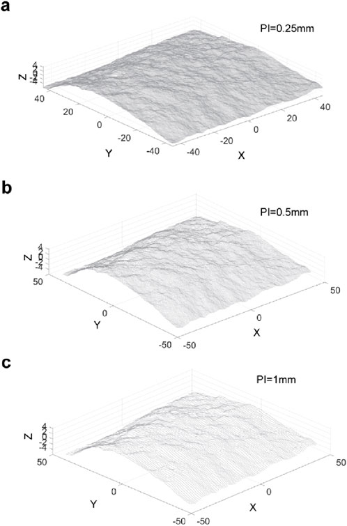
Figure 4. Point clouds of rock surface with profile intervals (PI) of (A) 0.25 mm, (B) 0.5 mm and (C) 1 mm respectively.

To validate the accuracy of roughness parameters at different shooting distances, a high-resolution point cloud of the rock surface was generated using an AutoScan-630W laser scanner with a precision of 0.05 mm and an average point spacing of 0.005 mm. The JRC values derived from this point cloud were used as the benchmark for comparison.

2.5 Machine learning algorithms

The prediction model’s input feature set includes three parameters: OSRE, spatial distance, and the checkpoint spatial error of point clouds at various shooting distances. These features, combined with the JRC error as the target output, create a comprehensive dataset. As shown in Figures 5–7, both the input and output parameters are based on actual measured data rather than a set of predetermined values. The core of this prediction task is a multivariate regression analysis, designed to explore the relationships between the input features and the target output. To achieve this, five machine learning models were utilized for predicting the JRC error. To ensure robust generalization and accurate predictions, the data was split using a 70/30 ratio: 70% of the data was randomly chosen as the training set for model development and parameter optimization, while the remaining 30% served as the validation set to independently assess the model’s predictive performance and mitigate overfitting (Liu et al., 2024). To ensure the convergence of generalization error in a more stable manner, K-fold cross-validation was employed (Fushiki, 2011). The training set was first divided into five subsets, each of which could serve as a validation set. Then, one subset was used for validation, and the process was repeated five times, with a different validation and training set used in each iteration.

Figure 5

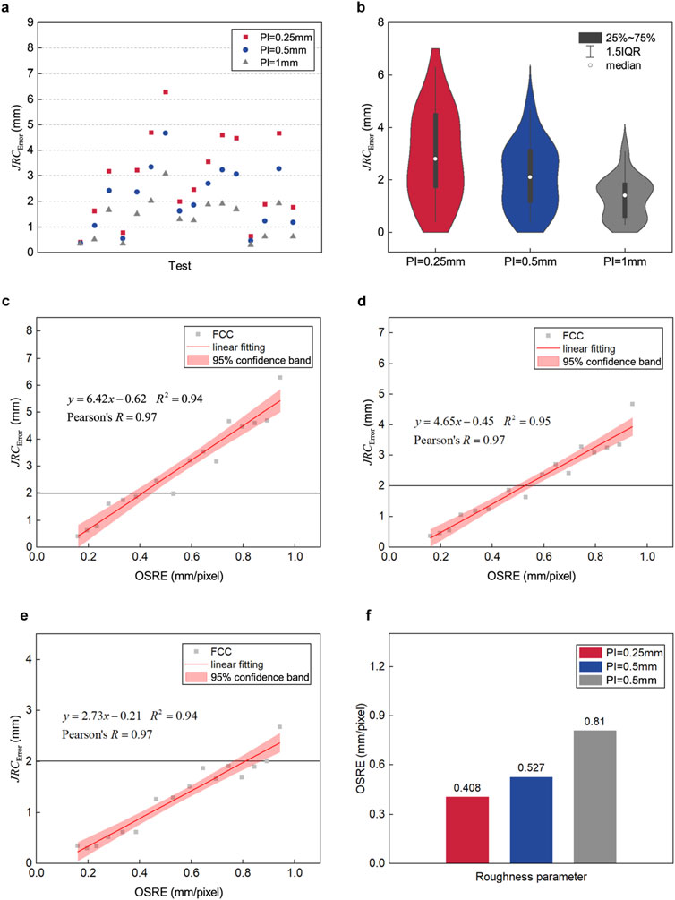
Figure 5. Overview of OSRE and $\mathit{J}R{C}_{\text{Error}}$ data results. (A) Distribution chart and (B) statistical chart of $\mathit{J}R{C}_{\text{Error}}$. The correlation between OSRE and $\mathit{J}R{C}_{\text{Error}}$ at PI of (C) 0.25 mm, (D) 0.5 mm and (E) 1 mm. (F) OSRE threshold values corresponding to $\mathit{J}R{C}_{\text{Error}}$ of 2.

Figure 6

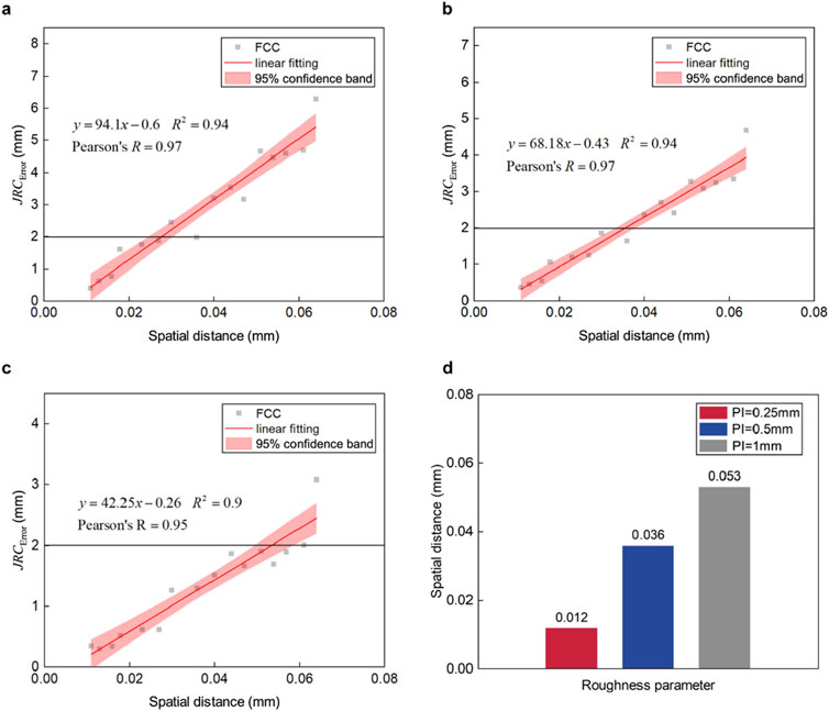
Figure 6. The correlation between spatial distance and $\mathit{J}R{C}_{\text{Error}}$ at PI of (A) 0.25 mm, (B) 0.5 mm and (C) 1 mm. (D) Spatial distance threshold values corresponding to $\mathit{J}R{C}_{\text{Error}}$ of 2.

Figure 7

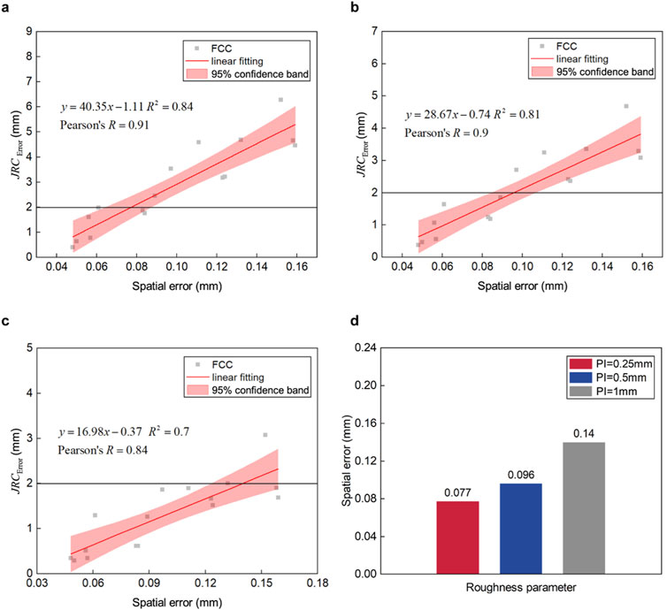
Figure 7. The correlation between spatial error and $\mathit{J}R{C}_{\text{Error}}$ at PI of (A) 0.25 mm, (B) 0.5 mm and (C) 1 mm. (D) Spatial error threshold values corresponding to $\mathit{J}R{C}_{\text{Error}}$ of 2.

2.5.1 Support Vector Regression

Support Vector Regression (SVR) is a technique rooted in Support Vector Machines (SVM) that models a regression function by identifying an optimal hyperplane within the feature space, enabling the projection of sample points into a higher-dimensional space. The objective of SVM is to find a function that places most data points within this margin while minimizing the prediction errors for the points that fall outside of it. These points, which fall outside the margin, are referred to as support vectors. Compared to traditional regression methods, SVR offers superior generalization ability and greater robustness, effectively handling high-dimensional data and nonlinear problems. The core idea of SVR is to balance the trade-off between prediction error and model complexity, adjusting hyperparameters to control the complexity and generalization capability of the model (Brereton and Lloyd, 2010; Awad et al., 2015). In this study, the kernel function was preset to quadratic, while the remaining hyperparameters were set to their default values.

2.5.2 Gaussian Process Regression

Gaussian Process Regression (GPR) is a statistical method used for predicting continuous values. The process begins with defining a prior distribution. A prior distribution is specified for the function to be predicted, assuming that this function adheres to a Gaussian Process with a zero mean function. Next, observation data, which includes input values and corresponding output values, are obtained. Following this, the posterior distribution is computed by updating the prior distribution with the observational data using Bayesian methods. The posterior distribution remains a Gaussian Process; however, its mean and covariance are adjusted based on the observational data. Finally, predictions are made by applying the posterior distribution to new input data. The prediction results are represented as a normal distribution, where the mean provides the predicted value and the variance indicates the uncertainty of the prediction (Williams and Rasmussen, 1995; Schulz et al., 2018). The kernel function for GPR in this study was preset to rational quadratic. The remaining hyperparameters are the default values.

2.5.3 Multilayer Perceptron

The Multilayer Perceptron (MLP) is a feedforward artificial neural network model, characterized by fully connected layers composed of multiple neurons. The architecture of MLP consists of several layers, including an input layer, hidden layers, and an output layer. The input layer receives data and forwards it to the hidden layers, where activation functions transform the input values into outputs, subsequently passed to the output layer. The output layer generates the final prediction. Each neuron in the hidden and output layers is associated with weights and biases, functioning as a nonlinear operator that processes inputs from preceding neurons through a series of computations to produce outputs. Information transmission between neurons in adjacent layers occurs through weighted connections, where the weights signify the strength of these connections. A key advantage of the MLP lies in its ability to model complex nonlinear relationships, making it suitable for regression tasks (Gardner and Dorling, 1998; Almeida, 2020). In this study, the MLP algorithm was implemented with a neural network architecture comprising three hidden layers, containing 25, 9, and 24 neurons, respectively. All other parameters were retained at their default values.

2.5.4 XGBoost

During each iteration, XGBoost reduces the objective function by incorporating an additional tree model. The objective function is composed of two elements: a loss function that quantifies the discrepancy between actual and predicted values, and a regularization term that manages model complexity to avoid overfitting. This balance ensures both reduced prediction errors and model simplicity. One of XGBoost’s defining features is the application of second-order Taylor expansion to approximate the loss function, thereby increasing the accuracy of the optimization process. Furthermore, a greedy algorithm is used to identify the best split points by evaluating changes in the objective function before and after the split, which enhances both the model’s accuracy and computational efficiency. Additionally, XGBoost’s capacity to automatically manage missing data offers a distinct advantage in handling complex datasets (Chen and Guestrin, 2016; Nielsen, 2016). In this study, the parameters for XGBoost were set as follows: n_estimators = 100, max_depth = 6, learning_rate = 0.03, subsample = 1, colsample_bytree = 1, and min_child_weight = 1, with all other hyperparameters set to their default values.

2.5.5 CatBoost

CatBoost is a gradient boosting framework utilizing symmetric decision trees, distinguished by its minimal parameter requirements, strong support for categorical variables, and high accuracy. Its key strength is the efficient handling of categorical features. Additionally, CatBoost effectively addresses gradient bias and prediction shift, reducing overfitting while improving both accuracy and generalization. Unlike XGBoost, CatBoost features an innovative algorithm that automatically converts categorical variables into numerical ones. This conversion starts with analyzing categorical features to determine the frequency of each category, followed by the use of hyperparameters to create new numerical features. CatBoost also enhances the feature space by combining categorical features and employs a ranking-based boosting method to handle noise in the training data, which helps to decrease gradient estimation bias and mitigate prediction shift (Hancock and Khoshgoftaar, 2020). In this study, the settings included iterations = 500, max_depth = 6, learning_rate = 0.09, with all other hyperparameters remaining at their default values.

3 Results

3.1 The relationship between OSRE and JRC

The accuracy of this study is evaluated using the difference ($JR{C}_{\text{Error}}$) between the JRC values obtained from laser scanning ($JR{C}_{3D}^{\text{Laser}\text{scanner}}$) and those obtained from photogrammetry ($JR{C}_{3D}^{\text{Photogrammetry}}$):

$JR{C}_{\text{Error}}=JR{C}_{3D}^{\text{Laser}\text{scanner}}-JR{C}_{3D}^{\text{Photogrammetry}}(6)$

The fitting results for $JR{C}_{\text{Error}}$ with profile intervals (PI) of 0.25 mm, 0.5 mm, and 1 mm are shown in Figure 5A. The image data reveal significant differences in the computed results under varying conditions. Figure 5B displays the error in $JR{C}_{\text{Error}}$ when the PI is 0.25 mm, 0.5 mm, and 1 mm, within the 25%–75% range. For PI = 0.25 mm, the error ranges from 1 to 5; for PI = 0.5 mm, the error ranges from 1 to approximately 3; and for PI = 1 mm, the error decreases to between 0 and 2. Such variations are evidently unreasonable and not acceptable based on the typical roughness profile classifications for JRC (Barton and Choubey, 1977). Consequently, an improvement in the accuracy of JRC measurements is necessary.

Figures 5C–E illustrate the relationship between OSRE and $JR{C}_{\text{Error}}$. Under the FCC strategy, instability arising from factors such as lighting conditions, image overlap, and handheld effects results in some variability in $JR{C}_{\text{Error}}$ values as OSRE increases, although a general linear correlation is evident. The 95% confidence interval bands indicate that most data points fall within this range, demonstrating a certain degree of linearity, though more precise validation is required. Pearson’s $R$, a measure of correlation between two datasets, can be used to analyze the relationship between OSRE and $JR{C}_{\text{Error}}$.

It is observed that, for PI values of 0.25 mm, 0.5 mm, and 1 mm, there is a strong correlation between OSRE and $JR{C}_{\text{Error}}$, with $R$ values approximately 0.97 in each case. The results show that $JR{C}_{\text{Error}}$ exhibits noticeable dispersion when OSRE is around 0.5–0.8. This is attributed to the larger spacing between points at higher OSRE values, resulting in sparser point clouds. Consequently, the estimated area becomes less stable when partitioned into grids.

Based on the correlation between the data, linear regression equations for OSRE and $JR{C}_{\text{Error}}$ were fitted. To better differentiate the goodness-of-fit across different PI values, $R^2$ was used as a parameter for comparing the regression model’s performance. As shown in Figures 5C–E, the fits for all three cases are quite good, with $R^2$ values of 0.94 for PI = 0.25 mm and 1 mm, and 0.95 for PI = 0.5 mm. This indicates a high level of correlation in all three scenarios.

For a deeper analysis of the impact of different profile intervals on the regression equations for OSRE and $JR{C}_{\text{Error}}$, the $JR{C}_{\text{Error}}$ boundary value was set to 2, according to the typical roughness profile classifications for JRC (Barton and Choubey, 1997). The OSRE values corresponding to this boundary represent the maximum shooting distance that meets the $JR{C}_{\text{Error}}$ requirements for each PI. In other words, a higher boundary OSRE value indicates a larger permissible shooting range for the equipment and greater tolerance. As shown in Figure 5F, OSRE values are 0.408 for PI = 0.25 mm, 0.527 for PI = 0.5 mm, and 0.81 for PI = 1 mm. Thus, the JRC accuracy reflected by OSRE varies to some extent with different contour line intervals.

3.2 The relationship between spatial distance and JRC

Figures 6A–C illustrate the fitting of spatial distance to $JR{C}_{\text{Error}}$ under different profile intervals. Similar to OSRE, a nearly linear relationship exists between spatial distance and $JR{C}_{\text{Error}}$, with $JR{C}_{\text{Error}}$ increasing as spatial distance grows. The results show that linear fitting is generally satisfactory across all three intervals. Quantitative analysis reveals that for PI = 0.25 mm and 0.5 mm, $R$ values are both 0.97 and $R^2$ values are 0.94. For PI = 1 mm, $R$ is 0.5 and $R^2$ is 0.9. Although there are slight differences from the OSRE results, the fitting quality is generally good across all intervals.

Figure 6D displays the boundary values for spatial distance under different profile intervals. For PI = 0.25 mm, the spatial distance is 0.012; for PI = 0.5 mm, it is 0.036; and for PI = 1 mm, it is 0.053. When PI = 0.5 mm, the boundary value is three times that of PI = 0.25 mm, and for PI = 1 mm, the difference in boundary value reaches up to 4.42 times. The JRC accuracy reflected by spatial distance exhibits significant variations across different profile intervals, underscoring the need to distinguish the precision impact patterns at each interval.

3.3 The relationship between spatial error and JRC

Figures 7A–C show the fitting of spatial error to $JR{C}_{\text{Error}}$, which can be approximated by a linear relationship, consistent with the behavior observed for OSRE and spatial distance. The results indicate that for PI = 0.25 mm, the fitting quality and correlation are the best, with $R$ of 0.91 and $R^2$ of 0.84. For PI = 0.5 mm, $R$ is 0.9 and $R^2$ is 0.81, while for PI = 1 mm, $R$ is 0.84 and $R^2$ is only 0.7. Therefore, among the three different intervals, PI = 0.25 mm and PI = 0.5 mm show the best results, whereas PI = 1 mm exhibits the poorest fitting quality. This suggests that spatial error can be used to characterize point cloud reconstruction as well as to represent estimation accuracy across different intervals.

Considering spatial error, the boundary spatial errors under different profile intervals are shown in Figure 7D. For PI = 0.25 mm, the spatial error is 0.077; for PI = 0.5 mm, it is 0.096; and for PI = 1 mm, it is 0.14. When PI = 0.5 mm, the boundary value is 1.25 times that of PI = 0.25 mm, and when PI = 1 mm, the boundary value is 1.82 times that of PI = 0.25 mm. Thus, the analysis of JRC estimation using spatial error across different profile intervals can also be extended for broader applications.

4 Discussion

4.1 JRC accuracy optimization model

In Section 3, an analysis of OSRE, spatial distance, and spatial error reveals a strong correlation between these three factors and $JR{C}_{\text{Error}}$. This study further examines the influence of these three factors across three different profile intervals, as shown in Figure 8A. The results indicate that the correlation between PI = 0.25 mm and PI = 0.5 mm is nearly perfect, with an $R$ value of 1. The relationship between PI = 1 mm and both PI = 0.25 mm and PI = 0.5 mm is also exceptionally strong, with $R$ values of 0.96 and 0.98, respectively. Additionally, the interrelationships of other factors are also depicted in the figure. Among these, OSRE shows a relatively stronger correlation across different profile intervals, with $R$ values of 0.97, 0.97, and 0.95. The impact of spatial distance and OSRE on different intervals is almost identical, while spatial error shows a weaker correlation compared to the other two factors, with $R$ values of 0.92, 0.90, and 0.84. Therefore, it can be concluded that, overall, the six data sets exhibit a very strong correlation, though there are still relative differences in influence among the different factors.

Figure 8

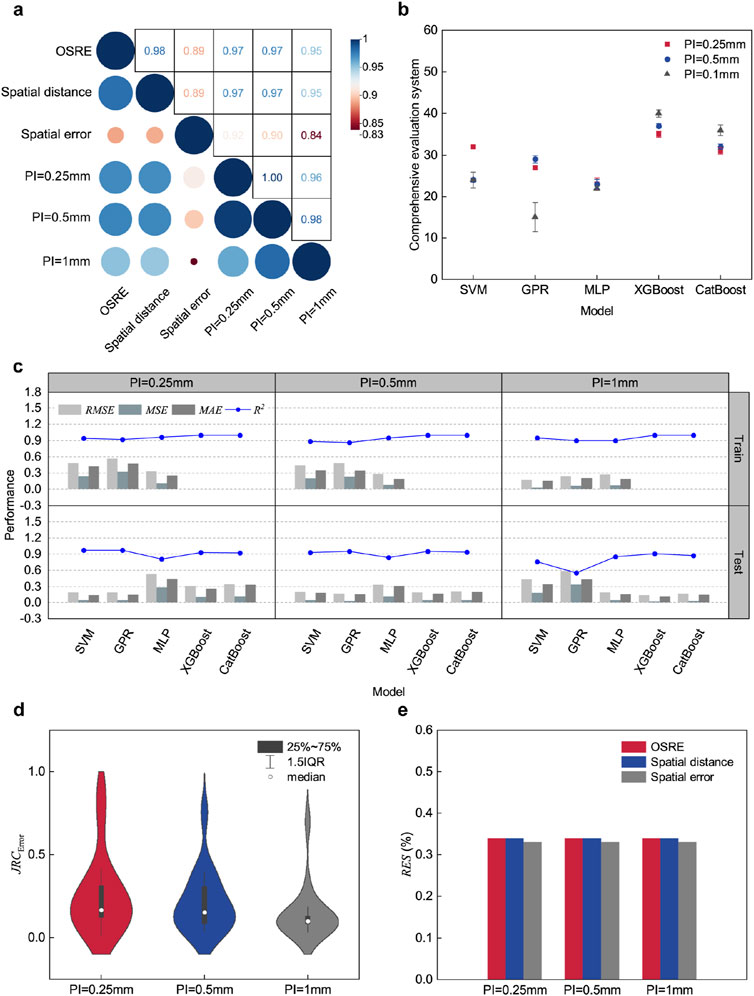
Figure 8. Training results of machine learning models: (A) Correlation analysis of OSRE, spatial distance, spatial error, PI = 0.25 mm, PI = 0.5 mm, and PI = 1 mm. (B) Comprehensive evaluation of machine learning models. (C) Performance evaluation of machine learning models. (D) Statistical distribution of optimized $\mathit{J}R{C}_{\text{Error}}$. (E) Sensitivity analysis of OSRE, spatial distance, and spatial error to $\mathit{J}R{C}_{\text{Error}}$.

Therefore, after applying five machine learning algorithms, the training and testing results of the models are shown in Figures 8B, C. $RMSE$, $MSE$, $MAE$, and $R^2$ are used as metrics to evaluate the model performance. Figure 8B illustrates the comprehensive performance of each model evaluated using the integrated assessment system (Zorlu et al., 2008). The difference in $R^2$ between the training and testing sets, scaled up by a factor of 10, is also depicted.

For PI = 0.25 mm, the highest overall score of 35 was achieved by the XGBoost model. SVM and CatBoost demonstrated similar scores of 32 and 31, respectively. Notably, SVM exhibited the smallest $R^2$ difference between the training and testing sets at 0.03, whereas XGBoost and CatBoost showed larger differences of 0.07 and 0.08, respectively. In comparison, GPR and MLP displayed weaker model performance, with overall scores of 27 and 23, and $R^2$ differences between training and testing sets of 0.05 and 0.15, respectively. These findings indicate that the XGBoost model outperformed the others, achieving the best overall performance despite its $R^2$ difference not being the smallest, as the difference remained within an acceptable range. The SVM model demonstrated strong performance as well, making it a viable option for this dataset. Conversely, GPR and MLP scored lower, reflecting their comparatively poor performance.

For PI = 0.5 mm, XGBoost achieved the highest overall score of 37, with the smallest $R^2$ difference between the training and testing sets at 0.05, indicating superior model performance. CatBoost ranked second with an overall score of 32 and an $R^2$ difference of 0.06, demonstrating good performance and stable data. In contrast, GPR, SVM, and MLP exhibited lower overall scores of 29, 24, and 23, respectively. Although the $R^2$ differences for these models were not substantial—0.09 for GPR, 0.05 for SVM, and 0.11 for MLP—their overall performance was comparatively poor.

When PI = 1 mm, the $R^2$ differences between the training and testing sets increased significantly across all models, ranging from 0.05 to 0.35, indicating heightened data instability at this interval. Overall, XGBoost demonstrated the best performance, achieving the highest total score of 40 and an $R^2$ difference of 0.09, making it the most suitable choice for predicting JRC errors. CatBoost performed reasonably well, with a total score of 36, though its $R^2$ difference was relatively larger at 0.13. The performance of the remaining models was less satisfactory.

The analysis indicates that the XGBoost model outperformed all others across all profile intervals, with $R^2$ differences between the training and testing sets ranging from 0.05 to 0.09, demonstrating strong stability. The CatBoost model ranked second in performance, with its overall scores increasing progressively as the profile interval expanded from 0.25 mm to 1 mm. The $R^2$ differences for CatBoost ranged from 0.06 to 0.13. This performance can be attributed to XGBoost’s ability to balance model complexity and prediction accuracy by incorporating additional tree models to minimize the objective function. Moreover, XGBoost exhibited robust performance in noisy environments and possessed the capability to automatically handle missing data, features that align well with the limited dataset size in this study. Additionally, as illustrated in Figure 8A, OSRE, spatial distance, and spatial errors displayed strong correlations, indicating a consistent influence of these factors, albeit with potential fluctuations as parameters varied.

The results obtained for PI values of 0.25 mm, 0.5 mm, and 1 mm were substituted into the XGBoost model, and predictions were made using different parameters. Subsequently, the errors between the predicted results and the standard results were recalculated using Equation 6, as illustrated in Figure 8D. It was observed that the $JR{C}_{\text{Error}}$ values across all three indicators ranged between 0 and 1, with average values below 0.5. The error ranges for PI = 0.25 mm and PI = 0.5 mm were similar, while the error for PI = 1 mm was slightly lower. The accuracy of JRC improved on average by 80.4%, 84.2%, and 89.5% for PI values of 0.25 mm, 0.5 mm, and 1 mm, respectively.

As a result, the performance of the trained machine learning model in predicting JRC errors based on OSRE, spatial distance, and spatial error is demonstrated. In practical applications, researchers can calculate OSRE using the formula proposed by Equation 1, while spatial distance and spatial error can be extracted from the point cloud as described in this paper. By inputting these three parameters into the XGBoost model, predicted $JR{C}_{\text{Error}}$ values can be obtained. These predicted $JR{C}_{\text{Error}}$ values can then be substituted into Equation 6, allowing for the reverse calculation of a JRC value that closely approximates the laser scanner estimate, thereby improving the accuracy of photogrammetric JRC estimation.

Additionally, to further evaluate the influence of OSRE, spatial distance, and spatial error on $JR{C}_{\text{Error}}$, the cosine amplitude method proposed by Yang and Zhang (1997) was employed, as shown in Figure 8E. It was evident that the $RES$ values under different profile intervals were very close, indicating that OSRE and spatial error had a greater impact on $JR{C}_{\text{Error}}$ compared to spatial distance. It can be observed that the sensitivity of $JR{C}_{\text{Error}}$ to the three parameters remains consistent across profile intervals of 0.25 mm, 0.5 mm, and 1 mm, with only numerical variations as the interval increases. The $RES$ of OSRE and spatial distance on $JR{C}_{\text{Error}}$ is identical, while the $RES$ of spatial error is only 0.01 lower than the other two.

4.2 Application scopes and limitations

This study highlights the practical application of photogrammetry techniques by validating an algorithm rooted in SfM principles to optimize shooting parameter selection. By automatically configuring the camera’s spatial arrangement based on equipment specifications, the algorithm streamlines the photogrammetry data collection process, offering accessible solutions for surveyors without expertise in computer vision. Additionally, the research presents a novel machine learning model designed to enhance the accuracy of JRC measurements. This model, particularly effective in fixed tripod scenarios, accurately predicts JRC errors across three distinct profile intervals, thus enabling more precise JRC estimations. Demonstrating both stability and adaptability, the model performs consistently well even under varying conditions, such as different shooting distances and lighting environments, underscoring its wide-ranging applicability.

While this study provides valuable insights, several limitations need to be addressed. A key limitation is the reliance on a dataset generated using specific data collection methods and equipment. Expanding the variety of strategies and tools in future studies could improve the generalizability of the findings. Additionally, the research is limited by a small sample size and a narrow range of data processing software. Testing the method across different rock sample sizes and employing various 3D reconstruction software would enhance its overall applicability. Therefore, it is advisable that when implementing the machine learning-based accuracy optimization method proposed in this study, the rock sample size and data processing environment should be closely aligned with those used in this research. Moreover, current methods for optimizing JRC accuracy have yet to be widely validated in engineering settings such as slopes and tunnels. Currently, parameters affecting and reflecting JRC accuracy have been limited to OSRE, spatial distance within the point cloud, and spatial error at checkpoints. The impact of additional factors, such as image overlap, the number of feature points in stereo matching algorithms, and lighting conditions, on JRC estimation accuracy remains unexplored. Future research should focus on comprehensive testing and analysis across a broader spectrum of engineering scenarios to achieve more precise and holistic performance evaluation and optimization.

5 Conclusion

A machine learning-based model for optimizing the accuracy of the JRC was proposed in this study, significantly enhancing the precision of JRC estimates at profile intervals of 0.25 mm, 0.5 mm, and 1 mm. Initially, the FCC strategy was applied within the SPSA framework to enable automatic selection of shooting parameters based on a fixed tripod strategy. This approach is adaptable to rock data acquisition scenarios guided by SfM principles. Subsequently, the correlations between OSRE, spatial distances in the point cloud, CPs’ spatial errors, and JRC errors were examined across different profile intervals. The findings indicate a strong correlation between OSRE, spatial distances, spatial errors, and JRC errors. Ultimately, this high correlation underpinned the development of a machine learning-based photogrammetry model for JRC accuracy optimization. This approach is particularly suited for fixed camera capture strategies, allowing for high JRC accuracy even at greater shooting distances or lower camera resolutions. Under the predictive capability of the XGBoost model, the accuracy of JRC improved on average by 80.4%, 84.2%, and 89.5% for profile interval values of 0.25 mm, 0.5 mm, and 1 mm, respectively.

Data availability statement

The original contributions presented in the study are included in the article/supplementary material, further inquiries can be directed to the corresponding author.

Author contributions

JY: Investigation, Methodology, Resources, Writing–original draft. QW: Investigation, Resources, Writing–review and editing. QY: Formal Analysis, Methodology, Software, Writing–review and editing. YF: Investigation, Resources, Writing–review and editing. WJ: Investigation, Resources, Writing–review and editing.

Funding

The author(s) declare that financial support was received for the research, authorship, and/or publication of this article. The authors acknowledge the financial support provided by the Key R&D Project in Shaanxi Province (No. 2024GX-YBXM-299) and the Research Funds of Department of Transport of Shaanxi Province (No.23-81X).

Conflict of interest

Authors JY, QW, YF, and WJ were employed by CCCC Second Highway Engineering CO., Ltd.

The remaining author declares that the research was conducted in the absence of any commercial or financial relationships that could be construed as a potential conflict of interest.

Publisher’s note

All claims expressed in this article are solely those of the authors and do not necessarily represent those of their affiliated organizations, or those of the publisher, the editors and the reviewers. Any product that may be evaluated in this article, or claim that may be made by its manufacturer, is not guaranteed or endorsed by the publisher.

References

Agisoft Metashape (2022). Agisoft Metashape User Manual Professional Edition, Version 2.2. Available at: https://www.agisoft.com/downloads/user-manuals/ (Accessed on August 21, 2024).

Google Scholar

Almeida, L. B. (2020). “Multilayer perceptrons,” in Handbook of Neural Computation (CRC Press), C1–C2. doi:10.1201/9780429142772

CrossRef Full Text | Google Scholar

American Society for Photogrammetry and Remote Sensing (ASPRS) (2015). ASPRS positional accuracy standards for digital geo-spatial data. Photogramm. Eng. Remote Sens. 81 (3), A1–A26. doi:10.14358/PERS.81.3.A1-A26

CrossRef Full Text | Google Scholar

An, P. J., Fang, K., Zhang, Y., Jiang, Y. F., and Yang, Y. Z. (2022). Assessment of the trueness and precision of smartphone photogrammetry for rock joint roughness measurement. Measurement 188, 110598. doi:10.1016/j.measurement.2021.110598

CrossRef Full Text | Google Scholar

Awad, M., Khanna, R., Awad, M., and Khanna, R. (2015). Support vector regression. Effic. Learn. Mach. Theor. concepts, Appl. Eng. Syst. Des., 67–80. doi:10.1007/978-1-4302-5990-9_4

CrossRef Full Text | Google Scholar

Barton, N. R., and Choubey, V. (1997). The shear strength of rock joints in theory and practice. Rock Mech. 10, 1–54. doi:10.1007/BF01261801

CrossRef Full Text | Google Scholar

Battulwar, R., Zare-Naghadehi, M., Emami, E., and Sattarvand, J. (2021). A state-of-the-art review of automated extraction of rock mass discontinuity characteristics using three-dimensional surface models. J. Rock Mech. Geotech. Eng. 13 (4), 920–936. doi:10.1016/j.jrmge.2021.01.008

CrossRef Full Text | Google Scholar

Brereton, R. G., and Lloyd, G. R. (2010). Support vector machines for classification and regression. Analyst 135 (2), 230–267. doi:10.1039/B918972F

PubMed Abstract | CrossRef Full Text | Google Scholar

Chen, T., and Guestrin, C. (2016). “Xgboost: a scalable tree boosting system,” in Proceedings of the 22nd acm sigkdd international con-ference on knowledge discovery and data mining. doi:10.48550/arXiv.1603.02754

CrossRef Full Text | Google Scholar

Cignetti, M., Godone, D., Wrzesniak, A., and Giordan, D. (2019). Structure from motion multisource application for landslide characterization and monitoring: The champlas du col case study, sestriere, North-Western Italy. Sensors 19 (10), 2364. doi:10.3390/s19102364

PubMed Abstract | CrossRef Full Text | Google Scholar

CloudCompare (2023). CloudCompare - open source project. Tutorials. Available at: https://www.danielgm.net/cc/ (Accessed June 20, 2023).

Google Scholar

Cultural Heritage Imaging (2015). Guidelines for calibrated scale bar placement and processing, Version 2.0. San Franc. CA Cult. Herit. Imaging. Available at: http://culturalheritageimaging.org/ (Accessed January 20, 2025).

Google Scholar

Edmund Optics (2023). Imaging optics resource guide. Section 6: Imaging Lens Selection Guide. Available at: https://www.edmundoptics.com/knowledge-center?query=&categoryid=33663&/ (Accessed on August 19, 2024).

Google Scholar

Fardin, N., Stephansson, O., and Jing, L. (2001). The scale dependence of rock joint surface roughness. Int. J. Rock Mech. Min. Sci. 38 (5), 659–669. doi:10.1016/S1365-1609(01)00028-4

CrossRef Full Text | Google Scholar

Francioni, M., Simone, M., Stead, D., Sciarra, N., Mataloni, G., and Calamita, F. (2019). A new fast and low-cost photogrammetry method for the engineering characterization of rock slopes. Remote Sens. 11 (11), 1267. doi:10.3390/rs11111267

CrossRef Full Text | Google Scholar

Fushiki, T. (2011). Estimation of prediction error by using K-fold cross-validation. Stat. Comput. 21, 137–146. doi:10.1007/s11222-009-9153-8

CrossRef Full Text | Google Scholar

García-Luna, R., Senent, S., and Jimenez, R. (2021). Using telephoto lens to characterize rock surface roughness in SfM models. Rock Mech. Rock Eng. 54 (5), 2369–2382. doi:10.1007/s00603-021-02373-7

CrossRef Full Text | Google Scholar

Gardner, M. W., and Dorling, S. R. (1998). Artificial neural networks (the multilayer perceptron)—a review of applications in the atmospheric sciences. Atmos. Environ. 32 (14-15), 2627–2636. doi:10.1016/s1352-2310(97)00447-0

CrossRef Full Text | Google Scholar

Ge, Y. F., Chen, K. L., Liu, G., Zhang, Y. Q., and Tang, H. M. (2022). A low-cost approach for the estimation of rock joint roughness using photogrammetry. Eng. Geol. 305, 106726. doi:10.1016/j.enggeo.2022.106726

CrossRef Full Text | Google Scholar

Ge, Y. F., Kulatilake, P. H., Tang, H. M., and Xiong, C. R. (2014). Investigation of natural rock joint roughness. Comput. Geotech. 55, 290–305. doi:10.1016/j.compgeo.2013.09.015

CrossRef Full Text | Google Scholar

Ge, Y. F., Tang, H. M., Huang, L., Wang, L. Q., Sun, M. J., and Fan, Y. J. (2012). A new representation method for three-dimensional joint roughness coefficient of rock mass discontinuities. Chin. J. Rock Mech. Eng. 31 (12), 2508–2517.

Google Scholar

Grasselli, G., and Egger, P. (2003). Constitutive law for the shear strength of rock joints based on three-dimensional surface parameters. Int. J. Rock Mech. Min. Sci. 40 (1), 25–40. doi:10.1016/S1365-1609(02)00101-6

CrossRef Full Text | Google Scholar

Hancock, J. T., and Khoshgoftaar, T. M. (2020). CatBoost for big data: an interdisciplinary review. J. Big Data 7 (1), 94. doi:10.1186/s40537-020-00369-8

PubMed Abstract | CrossRef Full Text | Google Scholar

Hartley, R. I., and Sturm, P. (1997). Triangulation. Comput. Vis. Image Und 68 (2), 146–157. doi:10.1006/cviu.1997.0547

CrossRef Full Text | Google Scholar

Isrm, I. (1978). Suggested methods for the quantitative description of discontinuities in rock masses. Int. J. Rock Mech. Min. Sci. and Geomech. Abstr. 15 (6), 319–368. doi:10.1016/0148-9062(78)91472-9

CrossRef Full Text | Google Scholar

Kong, D., Saroglou, C., Wu, F. Q., Sha, P., and Li, B. (2021). Development and application of UAV-SfM photogrammetry for quantitative characterization of rock mass discontinuities. Int. J. Rock Mech. Min. Sci. 141, 104729. doi:10.1016/j.ijrmms.2021.104729

CrossRef Full Text | Google Scholar

Lin, Q., Cao, P., Wen, G., Meng, J., Cao, R., and Zhao, Z. (2021). Crack coalescence in rock-like specimens with two dissimilar layers and pre-existing double parallel joints under uniaxial compression. Int. J. Rock Mech. Min. Sci. 139, 104621. doi:10.1016/j.ijrmms.2021.104621

CrossRef Full Text | Google Scholar

Lin, Q., Zhang, S., Liu, H., and Shao, Z. (2024). Water saturation effects on the fracturing mechanism of sandstone excavating by TBM disc cutters. Arch. Civ. Mech. Eng. 24 (3), 154. doi:10.1007/s43452-024-00964-z

CrossRef Full Text | Google Scholar

Ling, J. X., Li, X. J., Li, H. J., Shen, Y., Rui, Y., and Zhu, H. H. (2022). Data acquisition-interpretation-aggregation for dynamic design of rock tunnel support. Autom. Constr. 143, 104577. doi:10.1016/j.autcon.2022.104577

CrossRef Full Text | Google Scholar

Liu, Y. S., Li, A., Dai, F., Jiang, R., Liu, Y., and Chen, R. (2024). An AI-powered approach to improving tunnel blast performance considering geological conditions. Tunn. Undergr. Sp. Tech. 144, 105508. doi:10.1016/j.tust.2023.105508

CrossRef Full Text | Google Scholar

Nielsen, D. (2016). Tree boosting with xgboost-why does xgboost win every machine learning competition? Master Dissertation. Master's thesis. NTNU. http://hdl.handle.net/11250/2433761

Google Scholar

Paixão, A., Muralha, J., Resende, R., and Fortunato, E. (2022). Close-range photogrammetry for 3D rock joint roughness evaluation. Rock Mech. Rock Eng. 55 (6), 3213–3233. doi:10.1007/s00603-022-02789-9

CrossRef Full Text | Google Scholar

Patton, F. D. (1966). Multiple modes of shear failure in rock 1st ISRM Congress. Int. Soc. Rock Mech. Rock Eng. Lisbon, Portugal, September 1966.

Google Scholar

Schulz, E., Speekenbrink, M., and Krause, A. (2018). A tutorial on Gaussian process regression: modelling, exploring, and exploiting functions. J. Math. Psychol. 85, 1–16. doi:10.1016/j.jmp.2018.03.001

CrossRef Full Text | Google Scholar

Tse, R., and Cruden, D. M. (1979). Estimating joint roughness coefficients. Int. j. Rock Mech. Min. Sci. and Geomech. Abstr. 16 (5), 303–307. doi:10.1016/0148-9062(79)90241-9

CrossRef Full Text | Google Scholar

Williams, C., and Rasmussen, C. (1995). Gaussian processes for regression. Adv. Neural Inf. Process. Syst. 8.

Google Scholar

Xia, D., He, C., Tang, H. M., Ge, Y. F., Ma, J. W., and Zhang, J. R. (2022). An efficient approach to determine the shear damage zones of rock joints using photogrammetry. Rock Mech. Rock Eng. 55 (9), 5789–5805. doi:10.1007/s00603-022-02898-5

CrossRef Full Text | Google Scholar

Yang, Q. Z., Li, A., Dai, F., Cui, Z., and Wang, H. T. (2024). Improvement of photogrammetric joint roughness coefficient value by inte-grating automatic shooting parameter selection and composite error model. J. Rock Mech. Geotech. Eng. Accept. doi:10.1016/j.jrmge.2023.12.017

CrossRef Full Text | Google Scholar

Yang, Y., and Zhang, Q. (1997). A hierarchical analysis for rock engineering using artificial neural networks. Rock Mech. Rock Eng. 30 (4), 207–222. doi:10.1007/BF01045717

CrossRef Full Text | Google Scholar

Yong, R., Wang, C., Barton, N., and Du, S. (2024). A photogrammetric approach for quantifying the evolution of rock joint void geometry under varying contact states. Int. J. Min. Sci. Techno. 34, 461–477. doi:10.1016/j.ijmst.2024.04.001

CrossRef Full Text | Google Scholar

Yu, X. B., and Vayssade, B. (1991). Joint profiles and their roughness parameters. Int. J. Rock Mech. Min. Sci. and Geomech. Abstr. 28 (4), 333–336. doi:10.1016/0148-9062(91)90598-G

CrossRef Full Text | Google Scholar

Zorlu, K., Gokceoglu, C., Ocakoglu, F., Nefeslioglu, H. A., and Acikalin, S. (2008). Prediction of uniaxial compressive strength of sand-stones using petrography-based models. Eng. Geol. 96 (3-4), 141–158. doi:10.1016/j.enggeo.2007.10.009

CrossRef Full Text | Google Scholar