Studies of three dimensional stagged-grid finite difference for Z-axis tipper electromagnetic numerical simulation

ZTEM (Z-Axis Tipper Electromagnetic System) is a frequency-domain airborne electromagnetic exploration method that utilizes natural field sources. This method is highly efficient and capable of probing great depths, making it widely applicable in the exploration of polymetallic mineral deposits. However, large-scale 3D forward modeling faces computational challenges due to the increase in data volume. This study employs the Aggregation-based Algebraic Multigrid (AGMG) and staggered grid finite-difference methods to achieve rapid solutions for three-dimensional ZTEM problems. The study shows that the AGMG-CG algorithm requires fewer iterations and achieves faster solutions, significantly enhancing computational speed, especially for large-scale 3D forward modeling problems. By analyzing the forward response characteristics of ZTEM, we show that tipper data accurately reflect lateral electrical interfaces. Furthermore, through extensive model testing, we analyze the main factors influencing the forward response of ZTEM. The study reveals that topographical variations may produce false anomalies, that a reasonable data acquisition bandwidth is crucial for identifying anomalies at different depths, and that low-altitude flights yield better responses.

1 Introduction

ZTEM is a new technique developed based on the audio-frequency magnetotelluric method (AFMAG) and incorporating MT data processing techniques (Lo and Zang, 2008). This method observes natural magnetic field signals in the audio frequency range (25–720 Hz) and obtains tipper data based on the linear relationship between the horizontal (Hx, Hy) and vertical (Hz) components of the magnetic field in the frequency domain (Kuzmin et al., 2005; Lo and Zang, 2008). The tipper data is then inverted to obtain subsurface conductivity distribution information (Labson et al., 1985). Field observations for this method typically consist of ground-based measurements and aerial surveys. The ground-based measurements capture the orthogonal horizontal components of the magnetic field, while the vertical component is measured during aerial surveys across the study area (Legault et al., 2009). Therefore, compared to artificial source airborne electromagnetic methods (AEM), ZTEM has the advantage of greater exploration depth and reduces the labor and time costs associated with ground data collection (Sattel and Witherly, 2012). Since its introduction in 2006, the method has quickly found successful applications in mineral exploration (Lo and Zang, 2008; Pare et al., 2012). Legault et al. (2009), Sattel and Witherly (2012), and Pare et al. (2012) evaluated the ZTEM and AirMt systems through field tests, confirming their efficiency in detecting subsurface anomalies across geothermal and mineral-rich regions. Holtham and Oldenburg (2010) applied the Gauss-Newton inversion method to ZTEM data in Utah, effectively delineating the distribution of conductive and porphyry deposits. Soyer and Mackie (2018) study showed that ZTEM can refine MT data, enhancing resistivity information retrieval. Kaminski and Oldenburg (2012) demonstrated ZTEM’s superior resolution and penetration in kimberlite exploration compared to VTEM, marking its advantage in airborne electromagnetic surveys. However, compared to hardware advancements, the relatively lagging state of electromagnetic data processing and interpretation technology has, to a certain extent, constrained the rapid development of electromagnetic methods. Currently, previous achievements are primarily focused on two-dimensional data processing and interpretation (Prikhodko et al., 2024a), but actual geological conditions are challenging to conform to the assumptions of a two-dimensional model (Ji et al., 2018). Therefore, it is essential to develop three-dimensional inversion methods that are closer to the actual geological conditions.

Currently, numerical simulations of electromagnetic methods mainly include integral equation methods (Xiong, 1992; Ren et al., 2017), finite element methods (Huang and Dai, 2002; Kordy et al., 2016; Ansari and Craven, 2022), and finite difference methods (Tan et al., 2003; Varılsüha and Candansayar, 2018). Integral equation methods only require partitioning of the target area, which significantly reduces the number of grids and improves computational efficiency. However, for complex models, further improvements are needed in terms of solving difficulty and computational accuracy. Finite element methods are widely applied in three-dimensional electromagnetic numerical simulations due to their good adaptability to models. However, this method involves a large number of unknowns when forming linear equation systems, resulting in extensive computational load and long computation time. Similarly, finite difference methods can also handle complex models with faster solving speed and higher solution accuracy. Many geophysicists have conducted research on grid partitioning techniques and linear equation solving techniques to accelerate the forward process. These methods are now widely used in electromagnetic forward simulations (Yang et al., 2016; Li et al., 2012). Forward simulations ultimately require solving systems of equations, and the speed and accuracy of equation solving directly affect the computational precision and efficiency of the forward algorithm (Wu et al., 2010). Due to the large-scale nature of the linear equation systems in forward modeling, both direct solution methods and traditional iterative solvers experience a sharp increase in computation time as the model size grows, making them inadequate for meeting the demands of large-scale three-dimensional electromagnetic forward modeling problems. Among them, the Multigrid (MG) method, which originated in the 1960s, has a core advantage of being independent of grid scale in terms of convergence speed, maintaining stability even on highly discretized fine grids (Fedorenko, 1964). This characteristic makes it particularly effective in dealing with complex problems. Hackbusch’s research has demonstrated that for linear elliptic partial differential equations, the MG algorithm is optimal in computational efficiency, with computational effort growing linearly with the number of grid nodes (Hackbusch, 2013). The Algebraic Multigrid (AMG) method defines the selection of coarse grids and the transfer operators between grids based on the coefficient matrix of the fine grid. The flexibility of this approach allows it to adapt to complex computational regions and variable material properties, thus gaining widespread application in geophysics (Stüben, 1983). Geophysicists have applied multigrid methods in seismic exploration, DC resistivity methods, as well as magnetotellurics and controlled-source electromagnetic methods (Bunks et al., 1995; Gao et al., 2002; Chen et al., 2017; Yin, 2016). Researchers such as Lan (2015) and Chen et al. (2017) conducted comparative analyses of various combination solving strategies using AGMG as a preconditioning operator (V-AGMG, V-AGMG-CG, V-AGMG-GCR, K-AGMG-CG, K-AGMG-GCR). They found that the AGMG algorithm’s iteration speed is independent of grid partitioning, and its iteration error decreases rapidly, making it an efficient and fast iterative solution algorithm.

Therefore, this paper begins by providing a brief overview of the ZTEM detection system. Subsequently, the three-dimensional forward modeling of ZTEM is achieved using the Aggregation-based Algebraic Multigrid (AGMG) method. Through numerical simulations of geoelectric models at different scales, the computational efficiency of the AGMG technique is analyzed. The study investigates the response characteristics of typical geoelectric models and discusses the impact of topographic variations, anomalous body depths, and flight heights on ZTEM data. This analysis deepens our understanding of the response characteristics, laying the groundwork for anomaly interpretation.

2 ZTEM theory

2.1 ZTEM system

The ZTEM method shares the same natural field sources as magnetotellurics (MT), both of which utilize vertically incident plane waves. Within a certain range, the horizontal components of the magnetic field can be approximated as uniform. Therefore, the horizontal magnetic field across the entire study area can be represented using the horizontal magnetic field measured at a remote reference station (Sattel and Witherly, 2012). Consequently, the ZTEM tipper can be expressed as:

$H_{\mathrm{z}}\left(r\right)=T_{zx}\left(r,r_0\right)H_x\left(r_0\right)+T_{zy}\left(r,r_0\right)H_y\left(r_0\right)(1)$

where r represents the position of the vertical magnetic field’s aerial measurement, r₀ represents the position of the ground reference station, and T_zx and T_zy denote the vertical magnetic field transfer functions, also known as tippers.

We consider natural electromagnetic waves as plane waves, which can be decomposed into the equivalent effects of two orthogonal field sources, SX and SY. Under the polarization mode of the SX field source, the horizontal magnetic field components at the ground base station are denoted as H_x⁽¹⁾ and H_y⁽¹⁾, and the vertical magnetic field component in the air is denoted as H_z⁽¹⁾. Similarly, under the polarization mode of the SY field source, the horizontal magnetic field components at the ground base station are denoted as H_x⁽²⁾ and H_y⁽²⁾, and the vertical magnetic field component is denoted as H_z⁽²⁾ (Holtham and Oldenburg, 2012). Therefore, according to Equation 1, the vertical magnetic field components in the air for these two polarization modes are:

$H_z^{\left(1\right)}=T_{zx}{H}_x^{\left(1\right)}+T_{zy}{H}_y^{\left(1\right)}(2)$

$H_z^{\left(2\right)}=T_{zx}{H}_x^{\left(2\right)}+T_{zy}{H}_y^{\left(2\right)}(3)$

Solving the system of Equations 2, 3, the expression for the vertical magnetic field transfer function in the ZTEM method can be obtained as:

$T_{zx}=\frac{H_y^{\left(2\right)}{H}_z^{\left(1\right)}-H_y^{\left(1\right)}{H}_z^{\left(2\right)}}{H_x^{\left(1\right)}{H}_y^{\left(2\right)}-H_x^{\left(2\right)}{H}_y^{\left(1\right)}}(4)$

$T_{zy}=\frac{H_x^{\left(1\right)}{H}_z^{\left(2\right)}-H_x^{\left(2\right)}{H}_z^{\left(1\right)}}{H_x^{\left(1\right)}{H}_y^{\left(2\right)}-H_x^{\left(2\right)}{H}_y^{\left(1\right)}}(5)$

To more intuitively display the response characteristics of ZTEM tipper data, the components of the two tippers are integrated by calculating the transverse partial derivative to obtain a parameter that highlights more significant lateral conductivity changes. From Equations 4, 5, the divergence of the ZTEM tipper can be obtained, and it can be expressed as Equation 6:

$DT=\frac{\mathrm{\partial }{T}_{zx}}{\mathrm{\partial }x}+\frac{\mathrm{\partial }{T}_{zy}}{\mathrm{\partial }y}(6)$

2.2 Three-dimensional numerical simulation of ZTEM with staggered grid finite differences

Therefore, this paper starts with Maxwell’s integral equations.

$\begin{array}{l}\oint \mathit{{\rm H}}\cdot dl=\iint \mathit{J}\cdot dS=\iint \sigma \mathit{{\rm E}}\cdot dS\\ \oint \mathit{E}\cdot dl=\iint i{\mu }_0\omega \mathit{H}\cdot dS\end{array}(7)$

E: Electric field strength vector; H: Magnetic field strength vector; μ₀: Magnetic permeability in vacuum; σ: Electrical conductivity of the medium; J: Current density; dl: Closed loop; ds: Closed loop’s enclosed area.

The study area is discretized into several cubic grid cells using staggered grids. For any grid cell, we define the electric vector potential components along the edges of the cuboid, with the recording points at the midpoints of the edges. The magnetic vector potential components are defined at the center positions of the cuboid’s surfaces, As shown in Figure 1. After discretizing the study area using a hexahedral grid, Maxwell’s equations need to be discretized using finite differences. Therefore, based on the relationships between the magnetic field and current density, the electric field and current density, and the magnetic field and electromagnetic effects as described in Equation 7, we discretized along the xyz directions, then eliminated the current density and electric field components, ultimately deriving the Maxwell’s equations that depend solely on a single magnetic field component. Specifically, the magnetic field component Hx within the study area is only related to the surrounding 12 magnetic field components (Tan et al., 2003).

$\begin{array}{l}{C}_1\cdot H_x\left(i,j,k-1\right)+C_2\cdot H_x\left(i,j-1,k\right)+C_3\cdot H_x\left(i,j,k\right)+C_4\cdot H_x\left(i,j+1,k\right)+\\ C_5\cdot H_x\left(i,j,k+1\right)+C_6\cdot H_y\left(i,j-1,k\right)+C_7\cdot H_y\left(i+1,j-1,k\right)+\\ C_8\cdot H_y\left(i,j,k\right)+C_9\cdot H_y\left(i+1,j,k\right)+C_{10}\cdot H_z\left(i,j,k-1\right)+\\ C_{11}\cdot H_z\left(i+1,j,k-1\right)+C_{12}\cdot H_z\left(i,j,k\right)+C_{13}{H}_z\left(i+1,j,k\right)=0\end{array}(8)$

Figure 1

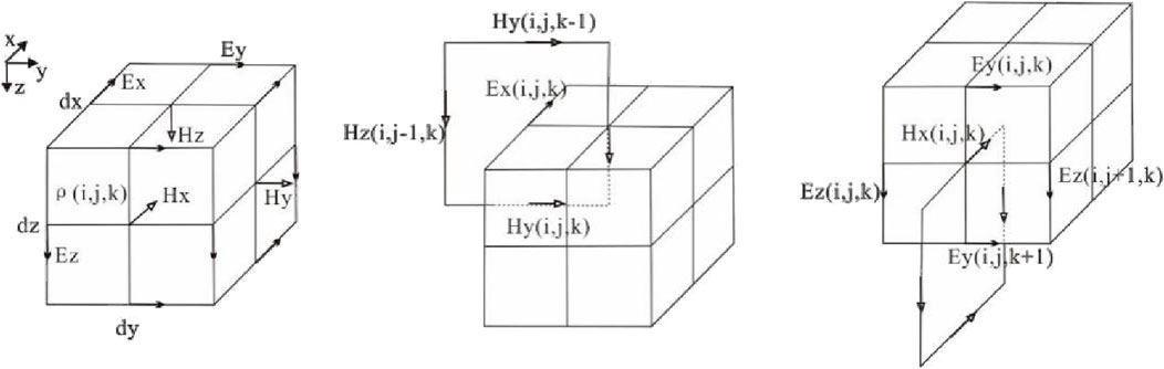
Figure 1. Staggered finite difference discretization with electric fields on cell edges and magnetic fields placed on cell faces.

Similarly, as with Equation 8, we can obtain the analogous expressions for Hy and Hz. Each component on the grid is calculated according to these three sets of equations, progressing step by step to the grid edges. The field values on the boundaries are given by the field sources, forming a large system of equations. In the entire solution domain, Hx has Nx (Ny-1) (Nz-1) unknowns to be solved, Hy has Ny*(Nx-1)*(Nz-1) unknowns, and Hz has (Ny-1)*(Nx-1)*Nz unknowns. We obtain a linear equation system for the magnetic field, which can be expressed as Equation 9:

$\mathit{A}·\mathit{{\rm H}}=\mathit{b}(9)$

A is a large complex sparse matrix, H represents the magnetic field components to be determined, and b is the right-hand side term related to the boundary conditions.

Where H represents the three components of the magnetic field, Hx,Hy and Hz, resulting in a total of Nx (Ny-1) (Nz-1)+ Ny*(Nx-1)*(Nz-1)+ (Ny-1)*(Nx-1)*Nz unknowns. Based on grid numbering, ordered sequentially by the indices i, j and k from small to large, b denotes the right-hand side corresponding to the magnetic field, while A represents the coefficient matrix. Since a specific unknown is only related to its neighboring 12 unknowns, each row in A will have only 13 nonzero elements, with all other elements being 0. Given the large scale of the sparse matrix, the speed of solving the linear equation system determines the speed of forward simulation, necessitating the use of optimized methods for solving.

The boundary conditions employ the first type of Dirichlet boundary conditions. Divergence correction techniques are commonly applied during the iterative solving process to enhance the speed and accuracy of solving this equation system.

2.3 Aggregated algebraic multigrid

In the process of forward modeling, the computation time and complexity of solving the equation system account for a substantial proportion of the entire numerical simulation (Wu et al., 2010). When using fine grid discretization to improve solution accuracy, the number of unknowns becomes very large. If general iterative methods such as Conjugate Gradient (CG) or Bi-Conjugate Gradient (BCG) are employed, their convergence is poor and they require a large number of iterations (Chen et al., 2017, Chen et al., 2018). In some cases, with the geometric increase of unknowns due to grid refinement, convergence may still not be achieved. To address these challenges, this section introduces the Aggregation-based Algebraic Multigrid (AGMG) method developed by Notay, 2010, accompanied by a related database. This method effectively mitigates the aforementioned solving issues and is considered the optimal approach for solving large linear equation systems (Notay, 2010; Notay, 2012; Napov and Notay, 2011).

The Algebraic Multigrid (AMG) method enhances the stability of the traditional AMG algorithm by achieving matrix coarsening through smooth aggregation based on matrix graph theory. This method consists of two main stages: aggregation coarsening and iterative solving. Matrix coarsening is a crucial part of multigrid methods (Lu et al., 2009). In algebraic multigrid, detached from grid geometry, achieves coarsening through algebraic matrix operations. A prolongation matrix P of size n × n_c is generated based on the coefficient matrix A to achieve matrix coarsening, where n_c is the number of coarsening variables and is less than n (Li et al., 2011). According to the Galerkin criterion (Notay, 2010), the coarse grid matrix can be obtained, which can be expressed as Equation 10:

${\mathit{A}}_c={\mathit{P}}^{\mathrm{T}}\mathit{A}\mathit{P}(10)$

Meanwhile, we define the transpose of the prolongation matrix as the restriction matrix.

In the process of aggregation coarsening, define set $G_i\left(i=1,\dots ,n_c\right)$ which can be geometrically considered as the nodes of the coarsened grid after mesh coarsening. G_i is disjoint from matrix A. The number of aggregation variables, n_c is then the number of elements in G_i. Thus, the prolongation matrix P can be expressed as Equation 11.

${\mathit{P}}_{ij}=\left\{\begin{array}{cc}1,& \text{\hspace{0.17em}if\hspace{0.17em}}i\in G_j\\ 0,& \text{\hspace{0.17em}other\hspace{0.17em}}\end{array}\right.\left(1\le i\le n,1\le j\le n_c\right)(11)$

In the equation, i represents the variable index of matrix A, and j represents the index of the aggregated variable set G_j. From this equation, it can be seen that the prolongation matrix P is a Boolean matrix, with at most one non-zero element per row. The coarse grid coefficient matrix, Equation 12, can be written as:

${\left({\mathit{{\rm A}}}_{\mathrm{c}}\right)}_{ij}={\left({\mathit{P}}^T\mathit{A}\mathit{P}\right)}_{ij}={\displaystyle \sum _{k\subset G_i}}{\displaystyle \sum _{l\subset G_j}}{a}_M,1\le i,j\le n_{\mathrm{c}}(12)$

i and j respectively represent the row and column indices of the coarse-grained coefficient matrix A_c.

In the AMG algorithm, the selection of the coarse-grid matrix A_c directly influences the stability and efficiency of the algorithm, making the construction of the extension matrix P crucial. This paper adopts the pairwise aggregation algorithm to construct the extension matrix (Notay, 2010). The algorithm achieves aggregation by regular covering of the matrix graph, clustering along the direction of the strongest connectivity. For any virtual grid node in the coefficient matrix A, pairing and aggregation are performed by identifying the strongest connected points (Muresan and Notay, 2008; Yin, 2016). To do so, the set of strongly connected points for virtual node i is defined first, which can be expressed as Equation 13:

${\mathit{S}}_i=\left\{j\ne i\left|a_{ij}<-\beta {\max }_{a_{\mu }<0}\right|a_{ik}\mid \right\}(13)$

In the equation, β represents the threshold for strong-weak connections, and its selection depends on the characteristics of the coefficient matrix A. For electromagnetic problems, β is typically chosen in the range of 0.4–0.6 (Chen et al., 2018). Therefore, the aggregation variable set can be expressed as Equation 14:

$G_i=\left\{\begin{array}{ll}\left\{i,j\right\},& \text{\hspace{0.17em}if\hspace{0.17em}}j\in S_j\\ i,& \text{\hspace{0.17em}other\hspace{0.17em}}\end{array}\right.\left(1\le i\le n_c\right)(14)$

In the multigrid algorithm, nested iterative techniques are crucial for connecting various grid layers or matrices. The V-cycle is one common cycling approach with relatively lower computational requirements. It efficiently smoothens the fine grid by applying the Gauss-Seidel iteration method to eliminate high-frequency errors. Subsequently, the residual error on the fine grid is restricted to the coarse grid using the restriction operator P^T, followed by coarse-grid calculations until a direct solution is achieved on the coarsest grid, providing an accurate numerical solution. Finally, the correction from the coarse grid is back-propagated through the interpolation operator P for solving on the fine grid until convergence is reached (Notay, 2010; Yin, 2016; Chen et al., 2018).

To address the challenges of the large sparse characteristics of the algebraic equation system in the finite-difference simulation of ZTEM and the difficulty of achieving good results with AGMG, especially in certain complex scenarios where solutions tend to diverge, a common approach is to combine the AGMG algorithm with conjugate gradient (CG) methods. Specifically, AGMG is utilized as a preconditioner for the conjugate gradient method, leveraging the advantage of AGMG’s lower iteration count and effectively reducing the condition number of the coefficient matrix. This hybrid approach accelerates the convergence rate of iterations and enhances the stability of the algorithm. We employ the conjugate gradient method (CG) as the Krylov subspace iterative algorithm, referred to as AGMG-CG. The main implementation process is as follows:

Input: Matrix A; Right-hand side b; Initial guess H₀; Maximum iterations m; Solution tolerance ε;

 Output: Approximate solution H_m; Residual: ${\mathit{r}}_m=\mathit{b}-\mathit{A}{\mathit{H}}_m$

 Initialize: ${\mathrm{r}}_0=\mathit{b}-\mathit{A}{\mathit{H}}_0$

For $j=1,2,3\dots \mathrm{m}$

 ${\mathit{z}}_j=Prec\left({\mathit{r}}_{j-1}\right)$

 ${\mathit{c}}_j^{\left(1\right)}=\mathit{A}{\mathit{z}}_j$

Loop i = 1,2,3 … j-1

 ${\gamma }_{ij}={\mathbf{c}}_i^T{\mathbf{c}}_j^{\left(i\right)},{\mathbf{c}}_j^{\left(i+1\right)}={\mathbf{c}}_j^{\left(i\right)}-{\gamma }_{ij}{\mathbf{c}}_i$

 ${\gamma }_{jj}=\parallel {\mathbf{c}}_j^{\left(j\right)}\parallel ;{\mathbf{c}}_j={\gamma }_{jj}^{-1}{\mathbf{c}}_j^{\left(j\right)}$

 ${\alpha }_j={\mathbf{c}}_j^T{\mathbf{r}}_{j-1};{\mathbf{r}}_j={\mathbf{r}}_{j-1}-{\alpha }_j{\mathbf{c}}_j$

 $\text{if}\parallel {\mathbf{r}}_j\parallel <\epsilon \parallel \mathbf{b}\parallel ,\text{exit}$ and m = j

 ${\mathit{H}}_m=\left[{\mathbf{z}}_1\dots {\mathbf{z}}_m\right]\left({\mathrm{\Gamma }}^{-1}\mathbf{a}\right)$

   $\mathbf{a}=\left[\begin{array}{c}{\alpha }_1\\ ⋮\\ {\alpha }_m\end{array}\right] and {\mathrm{\Gamma }}_{ij}=\left\{\begin{array}{l}{\gamma }_{ij},i\le j\\ 0,otherwise\end{array}\right.$

END

3 Computational efficiency analysis

To analyze the computational efficiency of the AGMG-CG algorithm, we selected the widely used Quasi-Minimal Residual (QMR) method (Siripunvaraporn et al., 2002). We compared the time required for both algorithms in 3D forward modeling. All algorithms in this paper were executed on a computer with an Intel Core i7-7700K 3.4 GHz processor, 16 GB of memory, and a 64-bit Windows 10 operating system. In 3D electromagnetic forward modeling, precise numerical methods are required, as analytic solutions are unavailable in three-dimensional cases. The accuracy of numerical simulations primarily depends on the grid discretization. In cases where the size of the modeling domain is fixed, using finer grids results in higher solution accuracy but increases the number of unknowns and computational load. Conversely, coarser grids reduce accuracy and may not provide accurate electromagnetic field values. Therefore, the size and number of grid elements are crucial factors in balancing computational accuracy and efficiency. In this study, we compared these two solving methods with grids of varying sizes. In the low-resistivity electrical model, four different grid sizes were designed while keeping the modeling domain constant: 32 × 32 × 42, 49 × 49 × 61, 84 × 84 × 96, and 114 × 114 × 126. We then employed the QMR and AGMG-CG algorithms to solve the airborne electromagnetic forward modeling for typical electrical models in the X-polarization and Y-polarization directions. With a period of 0.03 s and a flight altitude of 100 m, the relative error was solved to be 1.0E-8, and the decay curves for the iteration errors over iterations are shown in Figure 2.

Figure 2

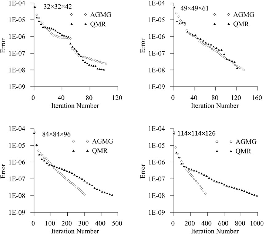
Figure 2. Comparison of computational efficiency of two algorithms under different grid sizes.

As depicted in Figure 2, the traditional QMR iterative algorithm exhibits swift decay in the initial iterations, displaying a relatively smooth error curve. Concurrently, with an escalation in the number of iterations, the error curve tends to plateau. Conversely, the Krylov subspace iterative algorithm AGMG-CG, employing AGMG preprocessing, displays a linear decay characteristic. With an augmentation in the number of iterations, its decay curve consistently maintains a linear trend. A comprehensive analysis of the iteration decay curves at different grid scales reveals that QMR exhibits a substantial increase in iteration counts with the growing number of grids, while AGMG-CG maintains an approximately linear and rapid descent as the number of grids increases, accompanied by a relatively slow increment in iteration counts. To further compare the computational efficiency of the algorithms, this study conducted a detailed analysis of the results for both methods across various grid quantities, as presented in Table 1. It is evident from the table that both approaches achieve the desired solution accuracy. For the small-scale grid of 32 × 32 × 42, the QMR algorithm exhibits fewer iterations and shorter forward simulation times. However, with an increase in the grid quantity, there is a significant escalation in the solution times and forward simulation times for both algorithms. This escalation is attributed to the increased computational load resulting from the expanded grid scale. In the case of the large-scale grid of 114 × 114 × 126, AGMG-CG demonstrates significantly fewer iterations and shorter solution times compared to the QMR algorithm. In summary, utilizing AGMG as a preconditioning operator at large grid scales offers the advantage of reduced iteration numbers and enhanced computational efficiency. Particularly in the case of large-scale exploration techniques such as ZTEM, The AGMG-CG algorithm ensures fast and stable computation processes.

Table 1

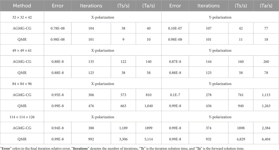
Table 1. Iterative results of different iterative algorithms for ZTEM forward modeling.

4 Model example

4.1 Typical electrical models

This section presents a low-resistivity electrical model as an example, which is advantageous for summarizing regularities and making method comparisons. This model exhibits a single response curve and is easy to understand. As shown in Figure 3, the geological body has dimensions of 2000 m in length, 2000 m in width, and 500 m in height. The top layer is buried at a depth of 250 m with a resistivity of 10 Ω m, while the background resistivity is 100 Ω m. The survey is conducted at a flight height of 100 m, with the base station located at (5000 m, 5000 m, 0). Ten periods ranging from 0.0001s to 0.03s, logarithmically spaced, are chosen for calculation. This electrical model uses Three-dimensional numerical simulations to compute tipper and divergence response maps.

Figure 3

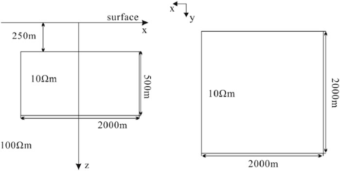
Figure 3. The sketch of Low-resistivity model.

Figure 4 shows the contour plots of the real and imaginary components of the tipper responses for different ZTEM components at 0.03s. The figures show that the real and imaginary components of the tipper response for the Tzx component create closed regions with symmetric positive and negative extreme anomalies at the boundaries of the low-resistivity zone in the x-direction. Moreover, at symmetric positions, the absolute values of the real and imaginary components of the tipper responses are equal, reflecting information about the low-resistivity boundary in the x-direction. Similarly, the Tzy component exhibits similar characteristics but reflects information about the low-resistivity boundary in the y-direction. The real and imaginary components of the tipper responses for Tzx and Tzy exhibit a good symmetric relationship at the boundaries of the anomalous body, with the anomaly range in the real part being smaller than that in the imaginary part. This indicates that the projection of low resistivity in the x-y plane lies between the maximum and minimum values, highlighting the high lateral resolution of the ZTEM tipper response.

Figure 4

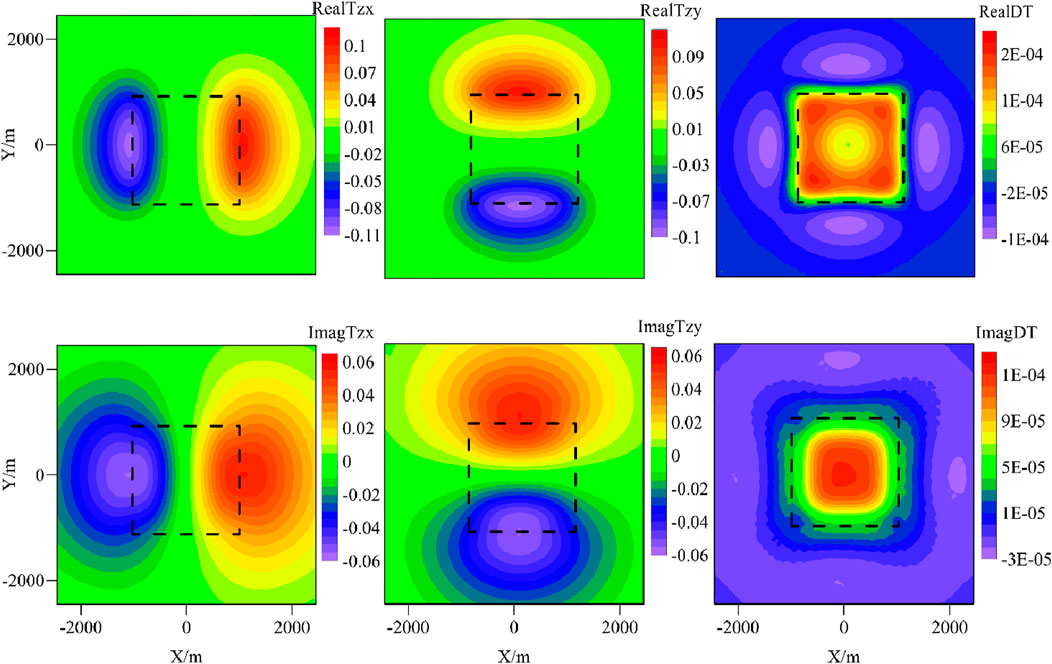
Figure 4. Imaging results of low-resistivity anomalies from the ZTEM system (the right image shows the real and imaginary parts of the tipper Tzx, the middle image presents the real and imaginary parts of the tipper Tzy, and the left image depicts the real and imaginary parts of the divergence DT).

After calculating the horizontal derivatives of Tzx and Tzy in their respective directions, a better representation of the contour information of the anomalous body in the x-y plane can be achieved. The real and imaginary responses of DT indicate that they display positive maxima at the center of the low-resistivity body, clearly revealing the position of the low-resistivity prism in the X-Y plane. This demonstrates that DT is better at reflecting the lateral distribution of the anomalous body’s position.

4.2 Analysis of influencing factors

4.2.1 Terrain influence analysis

Regardless of the detection method employed, the influence of topography cannot be ignored. To investigate the impact of terrain variations on the response of ZTEM data, this study designed three-dimensional models of mountain peaks and valleys, analyzing and discussing the responses at different frequencies and measurement points. Figure 5 illustrates the three-dimensional models of mountain peaks and valleys, where the mesa-shaped mountain peak has a relative height of 600 m, with a top base length of 500 m and a bottom base length of 2000 m. The valley has a relative depth of −600 m, with a top base length of 2000 m and a bottom base length of 500 m. The surrounding rocks underground have a resistivity of 100Ωm, and the resistivity of the air layer is 10^10 Ωm. Measurements were taken along a flight path 100 m above the mountain peak, with the base station located at (5000 m, 5000 m, 0). Ten logarithmically spaced periods were selected within the range of 0.0001s–0.03s. Through three-dimensional numerical simulations, the forward responses were obtained as shown in Figure 6.

Figure 5

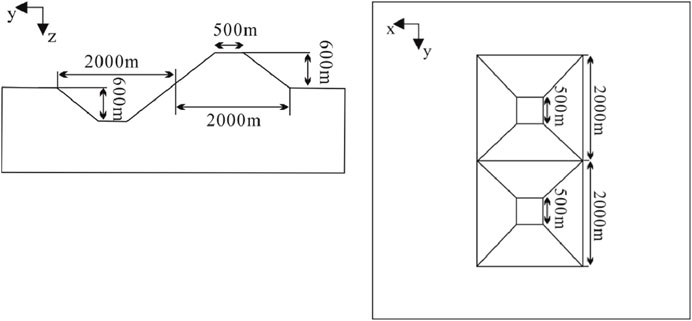
Figure 5. The sketch of model.

Figure 6

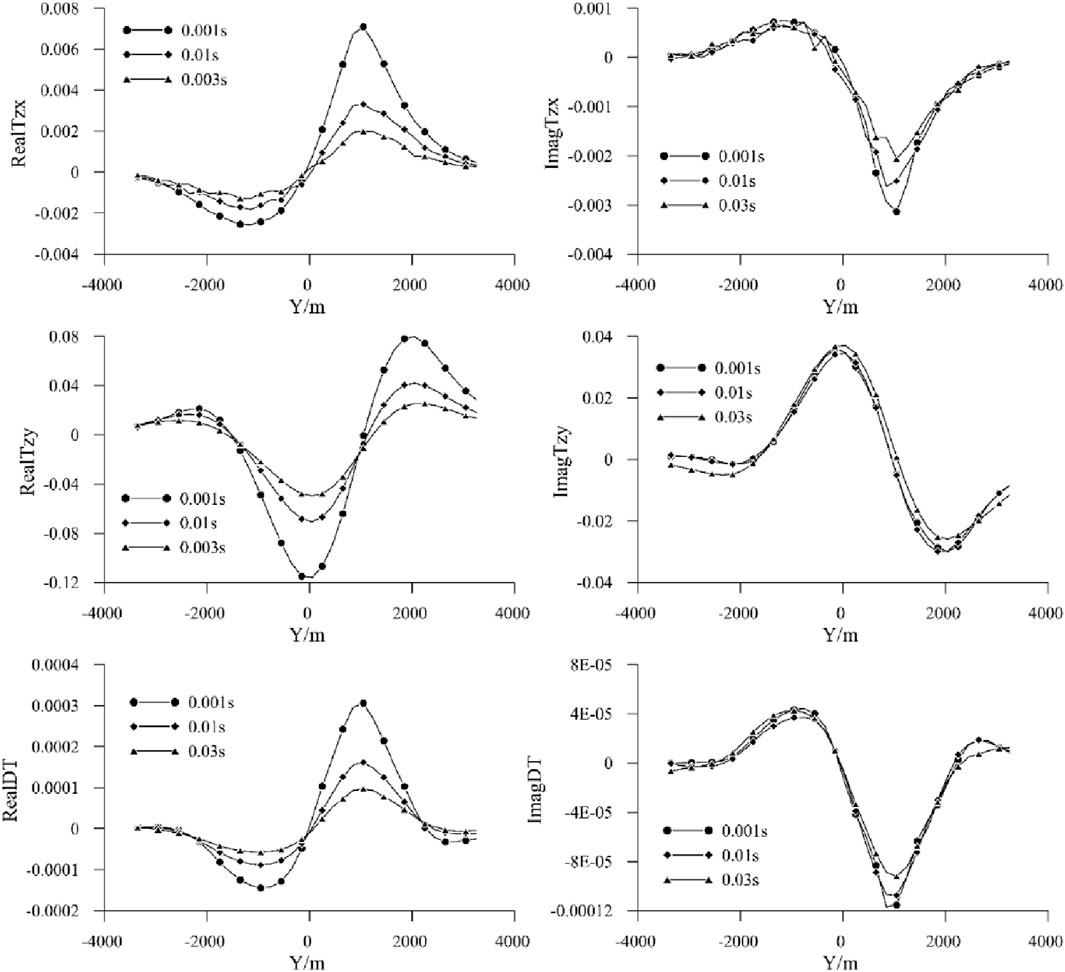
Figure 6. ZTEM response diagram for undulating topography at X = 50 m (the upper figure shows the real and imaginary parts of the tipper Tzx, the middle figure shows the real and imaginary parts of the tipper Tzy, and the lower figure shows the real and imaginary parts of the divergence DT).

In the tipper response shown in Figure 6, the real and imaginary parts of the tipper components Tzx, Tzy, and the divergence DT are influenced by undulating terrain, exhibiting gradual changes without abrupt variations. Whether in mountainous or valley terrain, both the real and imaginary parts of the three tipper components decrease with an increase in period, with relatively minor changes in the imaginary part of the tipper responses. The extreme points of Tzx and DT are located at the mountain peaks (valley bottoms), while in the tipper response of Tzy, the extreme points are mainly concentrated at the boundaries between the mountain peaks and valleys, especially in terrains with continuous variations from peaks to valleys. Furthermore, in the context of varying periods, the real part of the tipper response experiences more pronounced changes compared to the imaginary part, emphasizing the substantial impact of terrain. Therefore, in practical exploration, considering the terrain’s influence, particularly when assessing phase information during data processing, may yield more favorable outcomes.

4.2.2 Impact of anomalous body depth

Anomalous bodies exhibit different responses at varying depths. To enhance the quantitative analysis of their positions, in the previous section’s single low-resistivity model, burial depths of the low-resistivity anomaly were set at 50 m, 150 m, and 250 m, while keeping other parameters constant. The optimal observation period of 0.03s was selected for assessing the variations in tipper at different burial depths (as depicted in Figure 7).

Figure 7

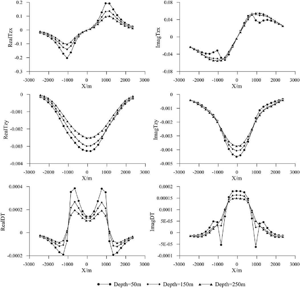
Figure 7. ZTEM response diagram for anomalous bodies at different depths at Y = 50 m (the upper figure shows the real and imaginary parts of the tipper Tzx, the middle figure shows the real and imaginary parts of the tipper Tzy, and the lower figure shows the real and imaginary parts of the divergence DT).

In Figure 7 with increasing burial depth of the low-resistivity anomaly, both the real and imaginary parts of Tzx gradually decrease only at the boundary of the target area, with overall small changes in the imaginary part. For Tzy, the real and imaginary parts decrease gradually at the center of the target area. The real and imaginary parts of DT exhibit significant variations at the boundary of the target area, with noticeable anomalies, and at the center of the anomaly, the amplitude decreases, although the magnitude of the change is small.

4.2.3 Impact of flight height

In three-dimensional scenarios, the effects of varying flight altitudes on ZTEM responses require further investigation. To explore this, a single low-resistivity electrical model was used with other parameters held constant, while flight altitudes were varied to [0 m, 100 m, 200 m, 500 m], and simulations were conducted to compare and analyze the response characteristics of ZTEM at different flight altitudes. For a clearer analysis, profiles were extracted along the X-direction (Y = 50 m), as shown in Figure 8, it can be observed that the poles of the tipper response (Tzx) correspond to the boundary positions of the anomalous body, while the extremum points of the Tzy response correspond to the center of the anomalous body in the X-direction. As the flight altitude increases, the amplitude of the tipper response gradually decreases, indicating an inverse relationship between the tipper response and flight altitude. The response curves under different flight altitude conditions exhibit consistent shapes, but with increasing altitude, the response range of the tipper becomes larger, leading to a reduced ability to identify boundary information. The divergence (DT) reveals that extremum points in the response correspond to the central position of the anomalous body, aiding in anomaly localization. It is recommended to maintain a low flight altitude during actual measurements as lower flight altitudes yield larger tipper amplitudes. Additionally, stable flight conditions are conducive to obtaining relatively stable data. To achieve high-precision results, using an altimeter for recording can facilitate amplitude correction and create favorable conditions for subsequent inversion calculations.

Figure 8

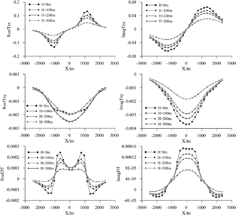
Figure 8. ZTEM response diagrams at different flight heights (the upper figure shows the real and imaginary parts of the tipper Tzx, the middle figure shows the real and imaginary parts of the tipper Tzy, and the lower figure shows the real and imaginary parts of the divergence DT).

5 Discussion

With advancements in airborne electromagnetic exploration instruments and the growing demand for refined and transparent three-dimensional geological exploration (Chang-Chun et al., 2015), the ZTEM has gained increasing favor due to its high efficiency and ability to probe great depths. However, the extensive detection area of ZTEM necessitates a greater subdivision of model units for detailed inversion interpretations. Under the current computational efficiency of existing forward modeling algorithms, conducting detailed inversion interpretations of full-area data remains challenging, even when utilizing the most advanced high-performance computers (Mengli et al., 2024). Consequently, rapid forward modeling research using ZTEM has become a focal point in the field of airborne electromagnetic exploration.

This study couples the Aggregation-based Algebraic Multigrid (AGMG) algorithm with the traditional Krylov subspace (CR) iterative algorithm to propose a novel AGMG-CG solving algorithm, which is applied for the first time to the forward modeling of ZTEM. This algorithm efficiently transforms large sparse equations from fine grids to coarser grids through several simple smoothing iterations, achieving effective solutions at a reduced computational cost, making it particularly suitable for large sparse matrix computations. Additionally, the algorithm demonstrates high convergence accuracy, speed, and computational efficiency. Compared to existing QMR programs, AGMG-CG can significantly enhance computational speed by several orders of magnitude, making it well-suited for large-scale three-dimensional forward modeling problems in airborne electromagnetic surveys (Wang et al., 2022; Xianyang et al., 2024).

The analysis of the ZTEM tipper and divergence indicates that this method can accurately reflect the lateral boundaries of anomalous bodies, which is crucial for geological exploration and mineral resource assessment (Sattel and Witherly, 2012). However, due to the lack of electric field information in the ZTEM tipper parameters, it is unable to effectively indicate the vertical boundaries of anomalous bodies. Currently, many researchers are employing joint inversion of ZTEM and MT to better constrain the vertical information of underground anomalies (Cao et al., 2023).

Additionally, this study explores various factors that influence ZTEM. The variations in topography significantly affect ZTEM data, and different types of terrain have differing impacts on these data. Results from case studies of undulating models indicate that the low-resistivity false anomalies caused by mountainous terrain and the high-resistivity false anomalies associated with valley terrain exhibit differing characteristics. At low frequencies, the impact of topography is relatively minor, while at high frequencies, the influence of topography is more pronounced. Therefore, it is essential to consider the effects of topography on data interpretation during exploration. This finding aligns with previous studies (Zhiqiang et al., 2021; Yue et al., 2017) in airborne electromagnetics, highlighting the importance of accounting for topography in data interpretation during exploration.

The burial depth and flight altitude have significant impacts on the identification of the boundaries of anomalous bodies. This is mainly due to the attenuation of electromagnetic waves during their propagation; deeper burial depths and higher flight altitudes lead to poorer identification results. Under specific conditions, the detection depth achievable by ZTEM can reach 1 km (Prikhodko et al., 2024b). Lower flight altitudes can obtain better imaging results, and the impact on the identification effect is relatively small when the flight altitude is within 100 m (Wang et al., 2023).

6 Conclusion

In this study, we began with Maxwell’s equations, discretized them using the staggered grid finite-difference method, and applied first-type Dirichlet boundary conditions to obtain a linear equation system for the electric field to be solved. Subsequently, we introduced a novel multigrid algorithm, the AGMG algorithm, to solve this linear equation system. The three-dimensional forward simulation of ZTEM is achieved. Conclusions drawn from the numerical simulation results are as follows:

ZTEM tippers and their divergence can accurately reflect the lateral boundaries of anomalous bodies. However, since the ZTEM tipper parameters lack electric field information, they cannot effectively indicate the vertical boundaries of anomalous bodies.

Analyzing the effects of terrain, depth of anomalous bodies and flight altitude on ZTEM responses, multiple cases demonstrate the following: mountainous terrain yields low-resistivity false anomalies, while valleys yield high-resistivity false anomalies; the depth of anomalous bodies affects the variation in amplitude, necessitating the selection of optimal observation bands for different depths; higher flight altitudes result in smaller responses, advocating for low-altitude flights to obtain high-quality data.

Data availability statement

The original contributions presented in the study are included in the article/supplementary material, further inquiries can be directed to the corresponding author.

Author contributions

YW: Formal Analysis, Methodology, Writing–original draft, Writing–review and editing. JQ: Formal Analysis, Writing–review and editing. TC: Software, Writing–review and editing. SZ: Resources, Writing–original draft. YL: Data curation, Writing–review and editing.

Funding

The author(s) declare that no financial support was received for the research, authorship, and/or publication of this article.

Conflict of interest

The authors declare that the research was conducted in the absence of any commercial or financial relationships that could be construed as a potential conflict of interest.

Publisher’s note

All claims expressed in this article are solely those of the authors and do not necessarily represent those of their affiliated organizations, or those of the publisher, the editors and the reviewers. Any product that may be evaluated in this article, or claim that may be made by its manufacturer, is not guaranteed or endorsed by the publisher.

References

Ansari, S. M., and Craven, J. A. (2022). A fully finite-element based model-space algorithm for three-dimensional inversion of magnetotelluric data. Geophys. J. Int. 233, 1245–1270. doi:10.1093/gji/ggac519

CrossRef Full Text | Google Scholar

Bunks, C., Saleck, F. M., Zaleski, S., and Chavent, G. (1995). Multiscale seismic waveform inversion. Geophysics 60 (5), 1457–1473. doi:10.1190/1.1443880

CrossRef Full Text | Google Scholar

Cao, X., Huang, X., Yan, L., Ben, F., and Li, J. (2023). 3D joint inversion of airborne ZTEM and ground MT data using the finite element method with unstructured tetrahedral grids. Front. Earth Sci. 10, 998005. doi:10.3389/feart.2022.998005

CrossRef Full Text | Google Scholar

Chang-Chun, Y., Xiu-Yan, R., Yun-He, L., Yan-Fu, Q., Chang-Kai, Q., and Jing, C. (2015). Review on airborne electromagnetic inverse theory and applications. Geophysics 80 (4), W17–W31. doi:10.1190/geo2014-0544.1

CrossRef Full Text | Google Scholar

Chen, H., Deng, J. Z., Yin, M., Yin, C. C., and Tang, W. W. (2017). Three-dimensional forward modeling of DC resistivity using the aggregation-based algebraic multigrid method. Appl. Geophys. 14 (1), 154–164. doi:10.1007/s11770-017-0605-1

CrossRef Full Text | Google Scholar

Chen, H., Yin, M., Yin, C., and Juzhi, D. (2018). Three-dimensional magnetotelluric modeling using aggregation-based algebraic multigrid method. J. Jilin Univ. (Earth Sci. Ed.) 48 (1), 261–270. doi:10.13278/j.cnki.jjuese.20160359

CrossRef Full Text | Google Scholar

Fedorenko, R. P. (1964). The speed of convergence of one iterative process. USSR Comput. Math. Math. Phys. 4 (3), 227–235. doi:10.1016/0041-5553(64)90253-8

CrossRef Full Text | Google Scholar

Gao, Y., Guo, H., and Zhou, W. (2002). Advances in the study of forward and inverse problems of wave equations using multigrid methods. World Geol. 21 (1), 4. doi:10.3969/j.issn.1004-5589.2002.01.018

CrossRef Full Text | Google Scholar

Hackbusch, W. (2013). Multi-grid methods and applications, Springer Science and Business Media 4.

Google Scholar

Holtham, E., and Oldenburg, D. W. (2010). Three-dimensional inversion of ZTEM data. Geophys. J. Int. 182 (1), 168–182. doi:10.1111/j.1365-246x.2010.04634.x

CrossRef Full Text | Google Scholar

Holtham, E., and Oldenburg, D. W. (2012). Large-scale inversion of ZTEM data. Geophysics 77 (4), 37–45. doi:10.1190/geo2011-0367.1

CrossRef Full Text | Google Scholar

Huang, L. P., and Dai, S. (2002). 3D electromagnetic field finite element calculation method under complex conditions. Earth Sci. 27 (06), 775–779.

Google Scholar

Ji, Z., Li, T., and Li, T. (2018). Research on 3D forward modeling of magnetotellurics based on fast pseudo-linear integral equation method. Progress in Geophy. 33 (2), 6.

Google Scholar

Kaminski, V., and Oldenburg, D. (2012). The geophysical study of Drybones kimberlite using 3D Time Domain EM Inversion and 3D ZTEM inversion algorithms. ASEG Ext. Abstr. 2012 (1), 1–4. doi:10.1071/aseg2012ab324

CrossRef Full Text | Google Scholar

Kordy, M., Wannamaker, P., Maris, V., Cherkaev, E., and Hill, G. (2016). 3-D magnetotelluric inversion including topography using deformed hexahedral edge finite elements and direct solvers parallelized on SMP computers–Part I: forward problem and parameter Jacobians. Geophys. J. Int. 204 (1), 74–93. doi:10.1093/gji/ggv410

CrossRef Full Text | Google Scholar

Kuzmin, P., Lo, B., and Morrison, E. (2005). Final report on modeling, interpretation methods and field trials of an existing prototype AFMAG system. Ontario, Canada: Ontario Geological Survey Misc Data Release 167, 1–75.

Google Scholar

Labson, V. F., Becker, A., Morrison, H. F., and Conti, U. (1985). Geophysical exploration with audiofrequency natural magnetic fields. Geophysics 50 (4), 656–664. doi:10.1190/1.1441940

CrossRef Full Text | Google Scholar

Lan, Z. L. (2015). Research on 3D numerical simulation of CSAMT based on aggregation algebraic multigrid method. Nanchang, China: East China University of Technology.

Google Scholar

Legault, J. M., Kumar, H., Milicevic, B., and Hulbert, L. (2009). “ZTEM airborne tipper AFMAG test survey over a magmatic copper-nickel target at Axis Lake in northern Saskatchewan,” in Society of Exploration Geophysicists. SEG Technical Program Expanded Abstracts 2009, 1272–1276. doi:10.1190/1.3255083

CrossRef Full Text | Google Scholar

Li, Y., Hu, X., Yang, W., Wei, W., Fang, H., Han, B., et al. (2012). Parallel computing study of 3D staggered-grid finite difference numerical simulation for magnetotellurics. Chin. J. Geophys. 55 (12), 4036–4043. doi:10.6038/j.issn.0001-5733.2012.12.015

CrossRef Full Text | Google Scholar

Li, X. K., Wang, W., and Liu, L. (2011). Application of multigrid algorithm in three-dimensional electromagnetic forward modeling. China Min. 20 (S1), 167–171.

Google Scholar

Lo, B., and Zang, M. (2008). Numerical modeling of ZTEM (airborne AFMAG) responses to guide exploration strategies. Seg. Tech. Program Expand. Abstr. 27 (1), 1098–1102. doi:10.1190/1.3059115

CrossRef Full Text | Google Scholar

Lu, J. J., Wu, X. P., and Spitzer, K. (2009). Multigrid method for 3D modeling of Poisson equation. Prog. Geophys. 24 (1), 154–158.

Google Scholar

Mengli, T., Yin, C., Bo, Z., Xue, H., Xiujuan, R., Yang, S., et al. (2024). Three-dimensional forward modeling of frequency-domain airborne electromagnetic data based on the multiscale finite element method. Chinese Journal of Geophysics 67 (04), 1656–1668. doi:10.6038/cjg2023Q0725

CrossRef Full Text | Google Scholar

Muresan, A. C., and Notay, Y. (2008). Analysis of aggregation-based multigrid. SIAM Journal on Scientific Computing 30 (2), 1082–1103. doi:10.1137/060678397

CrossRef Full Text | Google Scholar

Napov, A., and Notay, Y. (2011). Algebraic analysis of aggregation-based multigrid. Numerical Linear Algebra with Applications 18 (3), 539–564. doi:10.1002/nla.741

CrossRef Full Text | Google Scholar

Notay, Y. (2010). An aggregation-based algebraic multigrid method. Electronic transactions on numerical analysis 37, 123–146. doi:10.1016/0377-0273(76)90010-X

CrossRef Full Text | Google Scholar

Notay, Y. (2012). Aggregation-based algebraic multigrid for convection-diffusion equations. SIAM journal on scientific computing 34 (4), A2288–A2316. doi:10.1137/110835347

CrossRef Full Text | Google Scholar

Pare, P., Gribenko, A. V., Cox, L. H., Čuma, M., Wilson, G. A., Zhdanov, M. S., et al. (2012). 3D inversion of SPECTREM and ZTEM airborne electromagnetic data from the Pebble Cu–Au–Mo porphyry deposit, Alaska. Exploration Geophysics 43 (2), 104–115. doi:10.1071/eg11044

CrossRef Full Text | Google Scholar

Prikhodko, A., Bagrianski, A., Wilson, R., Belyakov, S., and Esimkhanova, N. (2024a). Detecting and recovering critical mineral resource systems using broadband total-field airborne natural source audio frequency magnetotellurics measurements. Geophysics 89 (1), WB13–WB23. doi:10.1190/geo2023-0224.1

CrossRef Full Text | Google Scholar

Prikhodko, A., Bagrianski, A., and Kuzmin, P. (2024b). Airborne natural total field broadband electromagnetics—configurations, capabilities, and advantages. Minerals 14, 704. doi:10.3390/min14070704

CrossRef Full Text | Google Scholar

Ren, Z. Y., Chen, C. J., Tang, J. T., Zhou, F., Chen, H., Qiu, L. W., et al. (2017). A new 3D magnetotelluric integral equation forward modeling method. Chinese Journal of Geophysics 60 (11), 4506–4515. doi:10.6038/cjg20171134

CrossRef Full Text | Google Scholar

Sattel, D., and Witherly, K. (2012). The modeling of ZTEM data with 2D and 3D algorithms. 82th Ann InternatMtg, SEG, Expanded Abstracts 2012, 1–5. doi:10.1190/segam2012-0219.1

CrossRef Full Text | Google Scholar

Siripunvaraporn, W., Egbert, G., and Lenbury, Y. (2002). Numerical accuracy of magnetotelluric modeling: a comparison of finite difference approximations. Earth, planets and space 54, 721–725. doi:10.1186/bf03351724

CrossRef Full Text | Google Scholar

Soyer, W., and Mackie, R. (2018). Comparative analysis and joint inversion of MT and ZTEM data. ASEG Extended Abstracts 2018 (1), 1–7. doi:10.1071/aseg2018abt5_2f

CrossRef Full Text | Google Scholar

Stüben, K. (1983). Algebraic multigrid (AMG): experiences and comparisons. Applied mathematics and computation 13 (3-4), 419–451. doi:10.1016/0096-3003(83)90023-1

CrossRef Full Text | Google Scholar

Tan, H. D., Yu, Q. F., John, F., and Wei, W. B. (2003). Numerical simulation of three-dimensional staggered grid finite difference of magnetotellurics. Journal of Geophysics (05), 705–711. doi:10.3321/j.issn:0001-5733.2003.05.019

CrossRef Full Text | Google Scholar

Varılsüha, D., and Candansayar, M. E. (2018). 3D magnetotelluric modeling by using finite-difference method: comparison study of different forward modeling approaches. Geophysics 83, WB51–WB60. doi:10.1190/geo2017-0406.1

CrossRef Full Text | Google Scholar

Wang, Y. F., Liu, J. X., Guo, R. W., Liu, R., Li, J., Chen, H., et al. (2022). Efficient three-dimensional magnetotelluric forward modeling based on geometric multigrid preconditioning technique. Chin. J. Geophy. 65 (05), 1839–1852. doi:10.6038/cjg2022P0110

CrossRef Full Text | Google Scholar

Wang, H. W., Yu, S. B., Guo, Y., and Zhou, H. G. (2023). Analysis of detection capability of semi-aerial frequency-domain electromagnetic tipper divergence. Geological Review 69 (S1), 412–414. doi:10.16509/j.georeview.2023.s1.180

CrossRef Full Text | Google Scholar

Wu, G., Hu, X. Y., and Liu, H. (2010). Progress in three-dimensional forward numerical simulation of CSAMT. Progress in Geophysics 25 (5), 1795–1801. doi:10.3969/j.issn.1004-2903.2010.05.037

CrossRef Full Text | Google Scholar

Xianyang, H., Yin, C., Yang, S., YunHe, L., Bo, Z., XiuYan, R., et al. (2024). Three-dimensional magnetotelluric inversion based on the multigrid algorithm Chinese. Journal of Geophysics 67 (08), 3150–3161. doi:10.6038/cjg2024R0724

CrossRef Full Text | Google Scholar

Xiong, Z. (1992). Electromagnetic modeling of 3-D structures by the method of system iteration using integral equations. Geophysics 57 (12), 1556–1561. doi:10.1190/1.1443223

CrossRef Full Text | Google Scholar

Yang, H. J., Pan, H. P., Meng, Q. X., and Guo, B. (2016). Study on the influence of conductive surrounding rock on borehole 3D transient electromagnetic response. Petroleum Geophysical Exploration 288-293, 302. doi:10.3969/j.issn.1000-1441.2016.02.015

CrossRef Full Text | Google Scholar

Yin, M. (2016). Research on 3D forward modeling of magnetotellurics based on aggregation algebraic multigrid method. Nanchang, China: East China University of Technology.

Google Scholar

Yue, Z., Xiu, L., Yipeng, W., Jianlei, G., and Youqiang, Z. (2017). Study on the characteristics of airborne transient electromagnetic responses under three-dimensional fluctuating topographic conditions. Chinese Journal of Geophysics 60 (01), 383–402.

Google Scholar

Zhiqiang, L., Yang, S., Tan, H., and Chengke, Z. (2021). Three-dimensional forward and inverse modeling of ZTEM tipper data with topography. Geophysical and Geochemical Exploration 45 (03), 758–767. doi:10.11720/wtyht.2021.1349

CrossRef Full Text | Google Scholar