- 1China National Logging Corporation, Xi’an, China
- 2School of Information and Communications Engineering, Xi’an Jiaotong University, Xi’an, Shaanxi, China
Precisely estimating the carbonate’s porosity is essential for subsurface reservoir characterization. However, conventional methods for obtaining porosity using either core measurements or logging interpretation are expensive and inefficient. Considering the sequence data feature of logging curves and the booming development of intelligent networks in geoscience, this study proposes a reliable and low-cost intelligent Porosity Prediction Transformer (PPTransformer) framework for reservoir porosity prediction using logging curves as inputs. PPTransformer network not only extracts global features through convolutional layers but also captures local features using Encoders and self-attention mechanisms. This proposed network is a data-driven supervised learning framework with a superior accuracy and robustness. The testing results demonstrate that compared to the Transformer network, Long Short-Term time series network, and support vector machine method, the PPTransformer framework exhibits the highest average correlation coefficient and determination coefficient indicators and the lowest root mean square error and absolute error indicators. Moreover, adding stratigraphic lithology as geological constraints to the PPTransformer framework further improves the prediction performance. This indicates that geological constraints will enhance network performance.
1 Introduction
Carbonate rocks are critical oil reservoirs that play a significant role in China’s oil and gas production enhancement stage. They are widely distributed in China, such as the Tarim Basin, Sichuan Basin, Ordos Basin, and North China. Therefore, carbonate reservoirs have become a prominent fossil resource in recent decades. Moreover, with the development of exploration technologies, low porosity low permeability carbonate formation buried in a deeper depth (e.g., >4,500 m) consequently draws our attention (Luo et al., 2021).
Porosity is the most significant parameter for reservoir characterization, reflecting the reservoir’s fluid storage capacity. Over the past few decades, geophysicists have extensively estimated porosity through many methods (Fu et al., 2017; Fan et al., 2012; Tian et al., 2010; An and Cao, 2018; Xi and Zhang, 1995; Ma et al., 2022; Richardson, 2018; Li K. W. et al., 2021; Kumar et al., 2022; Wu et al., 2016; Wu et al., 2021). Three main approaches have been employed: core sample measurements, complex empirical mathematical models, and machine learning (ML) techniques.
The most straightforward method of obtaining porosity is from core measurements (Li et al., 2012; Wang et al., 2015; Lian et al., 2013). In addition, well log and seismic data have been extensively used for porosity prediction. Although Well log data exhibit non-linear characteristics, the correlation between different well logs is only sometimes apparent due to the substantial heterogeneity of the formations and the complexity of geological conditions (Ju et al., 2012). On the other hand, seismic data are affected by noise, which weakens seismic features, necessitating effective noise reduction techniques to enhance correlations between different datasets (Chen et al., 2021; Li C. et al., 2021; Luo et al., 2018; Mou et al., 2015). Understanding the internal relationships between seismic/rock physics parameters and reservoir properties helps improve the accuracy of porosity predictions (An and Cao, 2018). Bachrach et al. proposed a data-driven Bayesian joint inversion method to estimate porosity in tight sandstone using seismic data, bypassing the complexities of rock physics modeling (Xi and Zhang, 1995). Zhao et al. developed an empirical model for predicting porosity, leveraging the Kozeny equation and partial least squares regression to analyze the relationship between porosity and rock composition (Zheng et al., 2017).
Researchers have developed mathematical and physical models to establish relationships between elastic parameters and reservoir properties (Ma et al., 2022; Richardson, 2018; Li K. W. et al., 2021) to obtain porosity more efficiently. Porosity estimating from physical models mainly relies on core measurements and rock physics theories. Most physical models are qualitatively built by analyzing reservoir parameters and elastic parameter sensitivity, thus limiting the feasibility (Wang et al., 2020; Bengio et al., 1994). However, the actual rock is extremely complicated. Therefore, mathematical methods are employed to characterize rock properties mathematically (Wu et al., 2021; Xiong et al., 2021; Zhang D. X. et al., 2018). However, mathematical models significantly rely on initial inputs. Consequently, physical modeling and mathematical methods cannot be widely adopted.
Due to their powerful data-fitting capabilities, machine learning methods have been used for porosity prediction in recent decades. ML techniques can automatically establish a non-linear relationship between well log/seismic data and reservoir parameters (e.g., porosity) with prior knowledge (Kumar et al., 2022; Wu et al., 2016; Wu et al., 2021). Numerous successful studies have demonstrated the powerful ability of ML techniques to explore correlations between multiple complex variables in geophysics. The most commonly used reservoir parameter prediction methods include Support Vector Regression (SVR), Random Forest (RF), and Artificial Neural Networks (ANN) (Zhang G. Y. et al., 2018; Ren et al., 2019; Karimpouli et al., 2010). Zhang et al. explored the non-linear relationship between porosity and rock physics parameters using SVR, demonstrating its better generalization than classical linear and multi-linear regression methods (Chen et al., 2022). Ao et al. proposed a linear random forest algorithm to predict porosity, showing its effectiveness in regression modeling through extensive experiments (Ao et al., 2019). Nkurlu et al. presented a neural network method for porosity prediction, which performed exceptionally well (Mathew Nkurlu et al., 2020). However, although these ML algorithms are functional for reservoir parameter prediction, the detailed processes are difficult to interpret physically, limiting their application. Enhancing data mining and interpretability in ML networks would help understand the non-linear relationships between input and output (Zhang et al., 2021).
Over the past decade, deep learning (DL) techniques have become even more potent than ML methods by stacking hidden layers and mapping them to higher-level representations to extract additional features from input data (Wu et al., 2018). Depending on whether labeled data are used to assist network training, DL methods can be categorized into supervised and unsupervised learning methods. With the increasing amount of data and improvements in computational hardware, DL techniques have been widely applied in geophysics, including for random and coherent noise attenuation (Yang et al., 2021), channel detection (Pham and Fomel, 2021), seismic data inversion (Kazei et al., 2021), and seismic event picking (Chen et al., 2019). Currently, the most popular DL techniques among geophysicists are based on Convolutional Neural Networks (CNNs) (Zhong et al., 2019) and Long Short-Term Memory (LSTM) networks (Hochreiter and Schmidhuber, 1997).
The advantage of CNNs lies in sharing parameters and local perception during network training, which allows us to extract local and global data features (Hinton and Salakhutdinov, 2006). Zhong et al. proposed a CNN model to predict reservoir parameters through logging curves (e.g., gamma-ray (GR), density (DEN), and shale content (SH)) as input (Wu et al., 2018). Feng et al. developed an unsupervised CNN method to invert acoustic impedance from seismic data and ultimately estimate porosity. This method improves lateral continuity using pre-trained weights from previous network layers to initialize subsequent hidden layers (Feng et al., 2020). Furthermore, LSTM, with its excellent ability to remember and extract long-term sequence features, has been widely used in deep sequence processing (Kalchbrenner et al., 2015; An and Cao, 2018; Ma et al., 2022; Wang et al., 2020). Chen et al. proposed a multi-layer LSTM (MLSTM) for porosity prediction and analyzed the impact of different well log inputs on prediction performance (Chen et al., 2020).
Recently, the Vision Transformer (ViT) framework has gained widespread attention across various fields due to its superior global feature extraction and parallel computing capabilities in natural language and image processing (Munchmeyer et al., 2021). ViT primarily consists of Transformer encoders (TEs) and decoders, with each encoder composed of self-attention (SA) mechanisms, layer normalization (LN), and feed-forward (FFW) layers. By reducing the distance between two positions in a sequence, ViT captures relationships between variables more effectively, thereby learning long-range dependencies. Compared to LSTM and CNN methods, ViT overcomes the limitations of parallel computing, allowing for the correlation of data features spanning longer ranges (Vaswani, 2017). Additionally, using attention mechanisms enhances the prediction performance and interpretability of the network.
In this paper, we design a PPTransformer framework for intelligent porosity prediction using well log data as input. Moreover, physical constraints are incorporated into the PPTransformer framework by using lithology as a geological constraint to assist in model training, further improving the prediction accuracy of the PPTransformer framework. The structure of the paper is as follows: first, the architecture and principles of the Transformer network are described. Second, the proposed PPTransformer framework is validated using actual data. Third, lithology is added as a constraint to enhance performance further. Finally, the results are discussed, and conclusions are drawn.
2 Methodology
2.1 Research workflow
Figure 1 illustrates the workflow for intelligent porosity prediction in carbonate reservoirs using the PPTransformer network. We can see that the entire workflow consists of data process, data separation, model configuration, model training, and test data validation.
(1) Feature selection: five well log curves (acoustic, gamma-ray, neutron, density, and resistivity logs) are selected as inputs to estimate porosity.
(2) Data preprocessing: the resistivity log is scaled logarithmically due to their significant magnitude difference from other logs.
(3) Dataset partitioning: the total dataset is from five wells. The two wells containing the most enormous data volumes are used for network training, while the remaining three are used for testing.
(4) PPTransformer configuration: the network comprises convolutional and Transformer encoder layers. The convolutional layers extract global features, while the encoder captures local features using multi-head self-attention mechanisms.
(5) Model training and porosity prediction: the model uses the Adam optimizer with RMSE as the loss function. It is then applied to the test dataset to evaluate its performance.
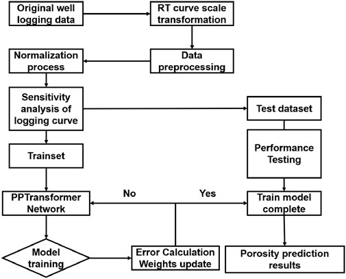
Figure 1. The identification process of carbonate porosity based on PPTransformer, including data filtering, feature selection, dataset division, model training, and testing.
2.2 PPTransformer structure
Traditional methods for porosity prediction mainly rely on well log data or seismic data. Similar to time series in natural language processing, well log data is a sequence recorded at fixed sampling intervals (e.g., 0.125 m) according to geological depth. Therefore, we propose a supervised deep learning framework that extracts important depth series features from input log data and establishes a non-linear mapping relationship between well log data and porosity. However, it is due to that the logging curves do not respond strongly to the porosity in the deeper depth. Therefore, we focus on extracting both global and local features when constructing this non-linear mapping. The proposed Porosity Prediction Transformer framework (PPTransformer) is mainly composed of two structures: a one-dimensional convolutional part (1D conv) and a Transformer Encoder part (TE). The former one-dimensional convolutional layer extracts global features from the input well log data, reassembling the depth sequence and enhancing prediction performance. The latter TE component with the MHA mechanism helps establish a robust local non-linear mapping between the input well log data and porosity. The specific network structure is illustrated in Figure 2.
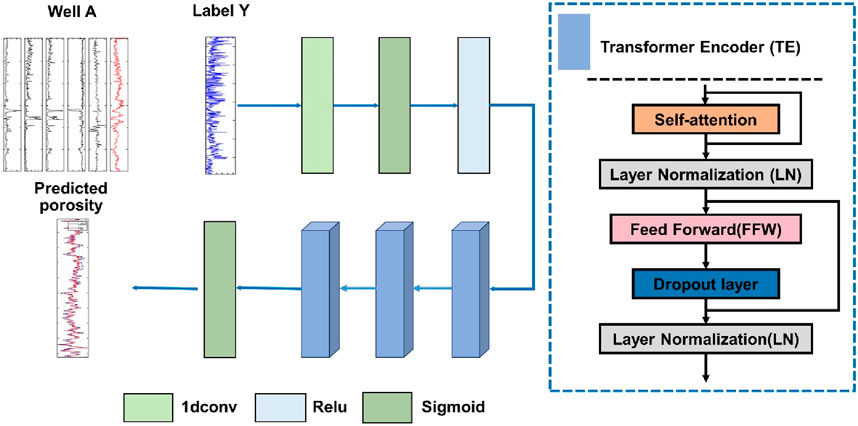
Figure 2. Framework of the proposed PPTransformer. It mainly includes a one-dimensional convolutional part and a Transformer Encoder part.
PPTransformer network can extract both global and local features during the porosity prediction. The one-dimensional convolutional layer with a Rectified Linear Unit (ReLU) is placed in the first layer to extract global features from the input well log curves. The output of this layer,
where
The most critical structure for the Transformer Encoder (TE) component is the Self-Attention (SA) mechanism. The SA mechanism reallocates weights to different parts of the input sequence to focus on essential features, thereby enhancing the relevance of positional embeddings. Each TE component comprises a standard SA block, two Layer Normalization (LN) blocks, one dropout layer, and a Feed-Forward Network (FFN). This paper constructs the PPTransformer using a Multi-Head Attention (MHA) mechanism based on the SA mechanism (Figure 2). A residual connection is added before the two LN layers (between the layer inputs and sublayer outputs) in the TE component. The global features extracted from the input are passed into the TE to extract local features. The crucial features from the previous layer are input into the attention mechanism, which generates three feature spaces and redistributes the weights. The three feature space matrices are the query (
The weight matrices
where
This process enhances the model’s capacity to learn complex representations while preserving the integrity of the original input data.
In the LN layer (Equation 5), the scaling and shifting parameters are denoted as γ and β, respectively.
Following LN1, a Feed-Forward Network (FFN) with two hidden layers is added. The first layer uses the ReLU activation function, while the second layer does not employ an activation function. The output of the FFN can be represented as Equation 6:
where
The PPTransformer framework first applies a one-dimensional convolutional layer to extract global features from the input well log curves. The extracted features are then passed into the TE component, where the MHA mechanism extracts robust features from the input sequence. Then residual structures enhance the learning capability from low-level to high-level feature representations. Finally, a fully connected layer with a Sigmoid activation function is set as the network’s last layer, outputting the predicted porosity.
The advantages of the PPTransformer framework can be summarized. First, the one-dimensional convolutional layer extracts global features from the input well log data, reassembling the depth sequence and enhancing prediction performance; second, the TE component with the MHA mechanism helps establish a robust non-linear mapping between the input well log data and porosity. The MHA mechanism allows the model to extract better features, reallocate weights to the underlying information, and improve the feature extraction capability.
3 Results and discussion
3.1 Data introduction
For data collection, the study area is divided into the Sangtamu Formation, Lianglitage Formation, and Yingshan Formation, with the Lianglitage and Yingshan Formations serving as the primary producing layers. The strata of the Lianglitage and Yingshan Formations are marginal and platform interior deposits, with the Lianglitage Formation exhibiting mud development and the Yingshan Formation consisting of pure limestone. The reservoir mainly underwent weathering and dissolution, forming large, highly porous cavernous reservoirs and highly heterogeneous, dense cave-type, fracture-cave-type, pore-type, and fracture-pore-type reservoirs.
The basic information on logging curves used in this study is shown in Table 1. A total of 15,294 sample points were collected from the five wells. According to the standard division for deep learning datasets, the training and test sets typically account for 80% and 20%, respectively. To improve the model’s robustness and generalization while maintaining the integrity of the well log curves, the two wells with the most enormous data volumes, Well A and Well C, were used as the training dataset, containing a total of 8,362 sample points, accounting for 54.67% of the overall data. The remaining three wells, Well B, Well D, and Well E, were used as the test dataset, containing 6,932 sample points, accounting for 45.32% of the overall data. Each well consists of five curves: acoustic time difference (AC), uranium-free gamma ray (CGR), neutron curve (CNL), density curve (DEN), and resistivity curve (RT). The label data is the porosity curve (POR) (Figure 3). According to the logging curve availability and sensitivity among input curves and porosity, the input well log data, including AC, CGR, CNL, DEN, and RT, are selected ultimately. From the rock physics perspective, the CGR curve reflects the clay volume, dominantly determining the formation type (e.g., shale, sandstone, carbonate). In addition, AC, CNL, and DEN curves are the most commonly used to interpret rock’s porosity during the petrophysical logging interpretation. Moreover, the RT curve is applied to interpret the fluid type in the pore volume. Therefore, geologically speaking, these five logging curves are most sensitive to rock porosity prediction.
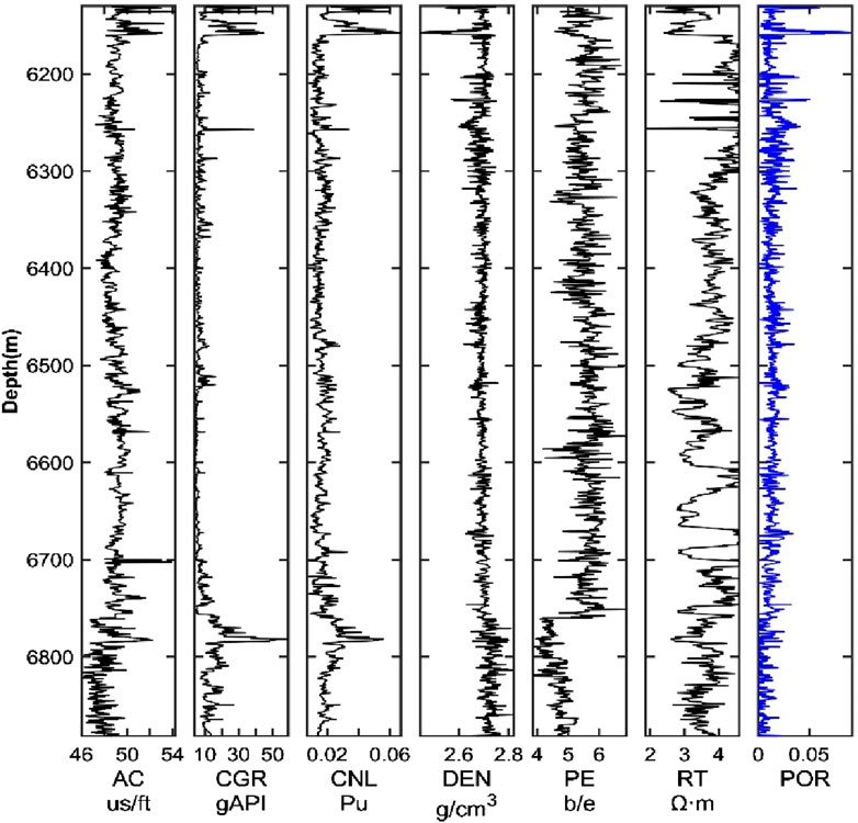
Figure 3. The training Well A’s logging curves include AC, CNL, DEN, CGR, and RT. Porosity is labeled.
3.2 Experimental process
The proposed PPTransformer network is a supervised learning framework that relies on well log data and actual labels to establish an implicit non-linear mapping relationship. The root mean square error (RMSE) loss function calculates the error between the actual labels and the predicted values during the training iterations. Various optimization methods were employed during the training phase to achieve optimal performance in porosity prediction. First, dropout and LN layers were used in the TE components to prevent overfitting during network training, with the dropout rate for all TE components set at 0.2. Second, the Adam optimizer was used to update parameters, with an initial learning rate of 1. Finally, an adaptive learning rate adjustment algorithm was employed to accelerate convergence and prevent overfitting. The learning rate decreases as the training epochs increase. The total number of training epochs was set to 300 (Figure 4). Specifically, after every 50 epochs, the learning rate was reduced to 0.1 times its previous value. When the validation loss did not decrease for 30 consecutive epochs, early stopping was applied to terminate training and save the best parameters. Due to the tight nature of carbonate reservoirs, the porosity values tend to be very low, and the original porosity values could not be used as labels for model training. Therefore, a scale transformation was applied to the porosity values, multiplying the overall porosity parameter by 100 and using the percentage values for model training. Correspondingly, when comparing results, the predicted values were divided by 100.
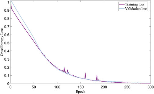
Figure 4. Loss curves of PPTransformer. It includes the training process (purple solid line) and validation process (grey solid line). The PPTransformer network starts to converge when reaching 250 epochs.
Figure 4 shows the loss curve of the model training. We can see that the model tends to converge after 250 epochs, with the final loss value of 0.02. During deep learning training models, the weak gradient signals of samples, noise, or small gradient changes may significantly cause short-term fluctuations (e.g., spikes in the loss curve) in the loss process. This situation is closely related to the characteristics and parameter settings of the neural network. Such spikes will disappear when the model converges ultimately.
3.3 Evaluation metrics
To quantify prediction error and evaluate the performance of the proposed method, Pearson’s correlation coefficient R, the coefficient of determination R2, RMSE, and mean absolute error (MAE) were used as evaluation metrics. Pearson’s correlation coefficient measures the correlation between two variables ranging from [−1,1]. Higher positive values indicate a stronger correlation, while negative values represent a negative correlation. The R2 value reflects the reliability of the variation in the dependent variable explained by the regression model, with values ranging from [0,1]. The larger values indicate better performance. RMSE measures the deviation between the predicted and actual values, with smaller values indicating lower error and better prediction performance. MAE is the average of the absolute deviations between each observed value and the arithmetic mean, with smaller values indicating better performance. The formulas for these four evaluation metrics are listed as Equations 8-11 as follows:
where
3.4 Results analysis
3.4.1 Results analysis for test dataset I
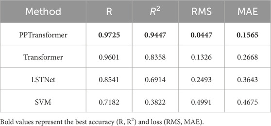
Test dataset I consists of the whole data points of Well B, with detailed information in Table 2. Three methods were used for benchmarking: a general Transformer network, a Long Short-Term Time Series Network (LSTNet), and a Support Vector Machine (SVM). Figure 5 shows the porosity prediction results and the five input well log curves. Intuitively, based on the magnitude of porosity values, the porosity curve can be divided into the upper (<6,050 m) and lower (>6,050 m) sections. The upper section has high porosity, while the lower section has low porosity. More importantly, the PPTransformer framework provides the best match between the actual and predicted porosity compared to other methods. In addition, we can see that all four methods capture the shape and trend of the porosity curve (blue label) and perform well in the low-porosity sections. However, the PPTransformer has the slightest error between predicted and actual values, while the SVM and Transformer methods exhibit underfitting in the high-porosity sections.
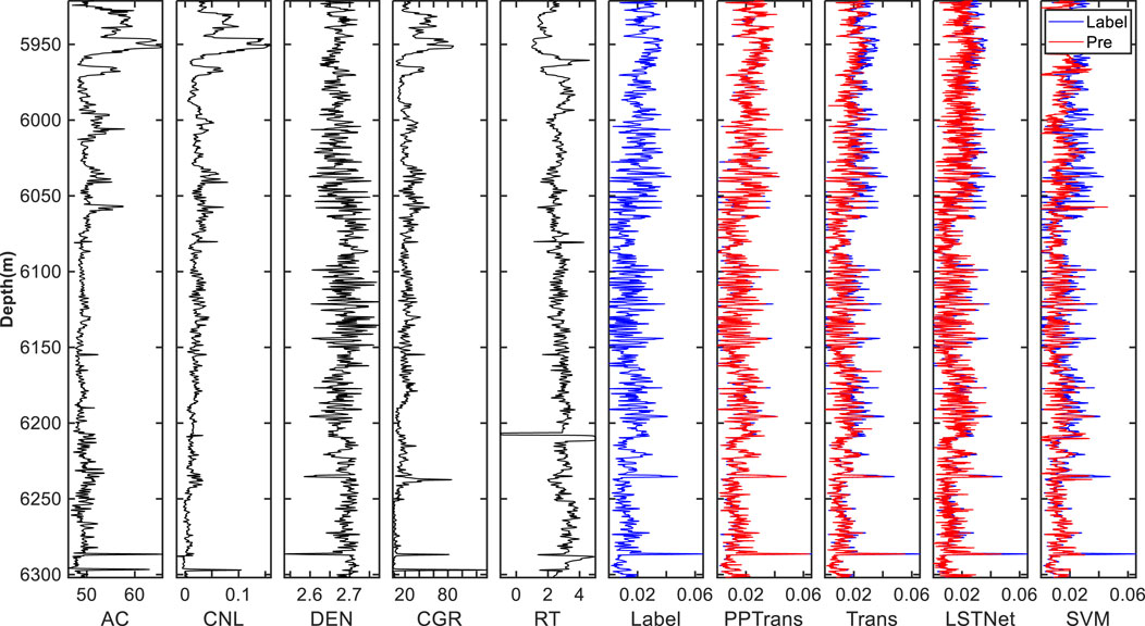
Figure 5. Comparison of porosity prediction results using different methods (e.g., PPTransformer, Transformer, LSTNet, SVM) on dataset I. The input logging curves include AC, CNL, DEN, CGR, and RT.
In addition, several evaluation metrics were used to quantify the prediction results (Table 2). Regarding evaluation metrics, PPTransformer achieves the highest R and R2 and the lowest RMSE and MAE compared to the benchmark methods, indicating that it has the highest accuracy and the lowest error. Figure 6 shows the cross-plots of porosity predictions using the four methods. The results of the PPTransformer and Transformer are consistent with the slope. In contrast, the results of LSTNet have more significant oscillations around the reference line, indicating a more substantial deviation. The SVM method results show only marginal consistency with the slope. Based on the cross-plots, residual and error histograms were plotted further to analyze the error of different porosity prediction methods.
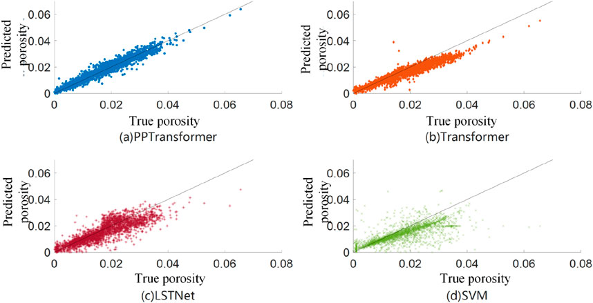
Figure 6. Cross plot porosity results from different methods on dataset I. (A-D) represent PPTransformer, Transformer, LSTNet, SVM, respectively.
3.4.2 Results analysis for test dataset II
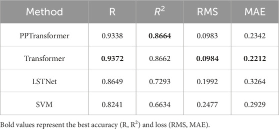
The proposed method and three comparison methods were further applied to test dataset II. Test dataset II consists of the whole data points from Well D. Figure 7 shows porosity prediction results and the five input well log curves. Intuitively, the PPTransformer framework and the general Transformer model provide the best fit between the actual and predicted porosity among the various methods. Both the LSTNet and SVM methods exhibit a underfitting in the middle and lower sections of the well. Table 3 shows that PPTransformer and Transformer achieved the highest R and R2 values and the lowest RMSE and MAE values. It implies that PPTransformer and Transformer’s performance on Dataset II is nearly identical. Figure 8 shows the cross-plots of porosity predictions using the four methods on Dataset II. The predicted results from both PPTransformer and Transformer align well with the reference slope. The predicted porosity from LSTNet presents more significant oscillations than the reference line, and the SVM method exhibits the most extensive oscillation range.
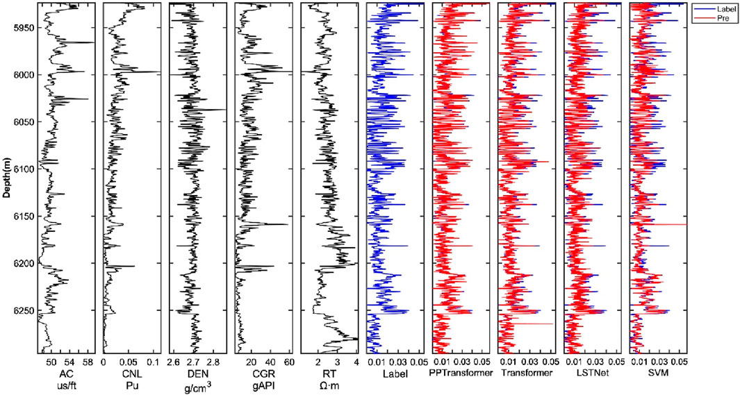
Figure 7. Comparison of porosity prediction results of 4 methods on dataset I. Including 5 input logging curves (AC, CNL, DEN, CGR, RT); methods include Transformer, LSTNet, and SVM.
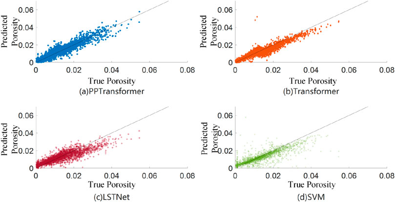
Figure 8. Cross plot porosity results from different methods on dataset II. (A-D) represent PPTransformer, Transformer, LSTNet, SVM, respectively.
3.4.3 Results analysis for test dataset III
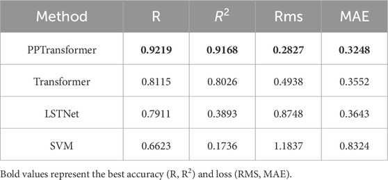
Finally, the four methods were applied to test dataset III, which consists of all the data points from Well E. Figure 9 shows the four methods’ porosity prediction results and the five input well log curves. Table 4 shows that PPTransformer achieved the highest R and R2 values and the lowest RMSE and MAE values. Intuitively, the general Transformer model provides the best fit between actual and predicted porosity. In most sections of Well E, the PPTransformer and LSTNet methods exhibit a smaller oscillation range, and the PPTransformer predictions appear less stable than those from the Transformer and LSTNet methods. The SVM method performed the worst on Well E, not only compared to the other three methods but also compared to its performance on Wells B and D. In most sections of the well, the SVM method showed severe underfitting, failing to predict the shape and trend of the porosity curve, and its expected values were far from the baseline. Similar to Wells B and D, Well E’s data was divided into four segments based on its length, with each segment containing approximately 500 sample points due to the smaller data volume in Well E compared to Wells B and D.
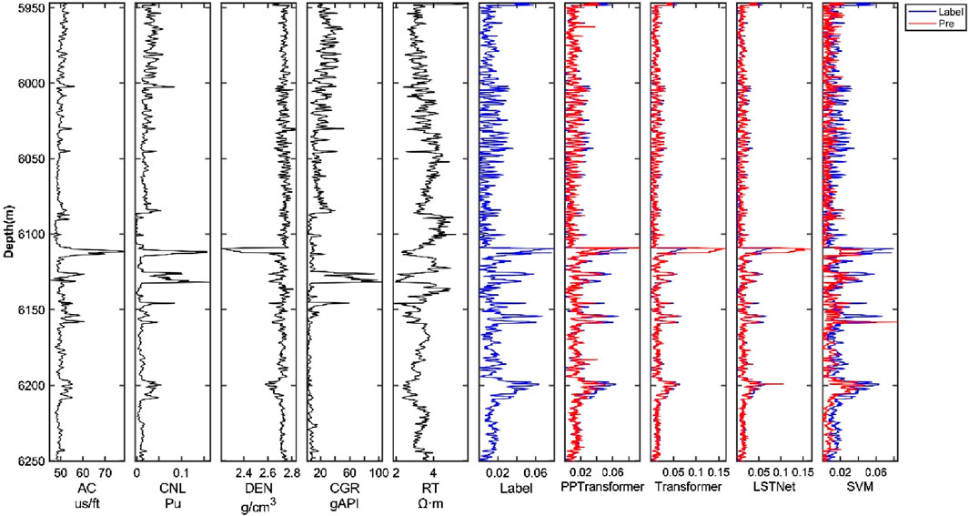
Figure 9. Comparison of porosity prediction results of 4 methods on dataset III. The input curves include AC, CNL, DEN, CGR, and RT; methods include Transformer, LSTNet, and SVM.
The cross plots of predicted and actual porosity using the four methods are shown in Figure 10. Interestingly, the results from Transformer and LSTNet are more concentrated, with the scatter points closer to the slope line. However, a few points deviate significantly, indicating more significant prediction errors for these points. Considering the low actual porosity values, these points will own a relatively high misfit, contributing to the fact that the evaluation metrics for Transformer and LSTNet are worse than those for PPTransformer. The predicted porosity from PPTransformer overall are outstanding, with very few points having significant errors. It explains its superior performance in the four evaluation metrics. The SVM method’s prediction results were poor, not only worse than the other three methods but also significantly worse than its performance on Wells B and D.
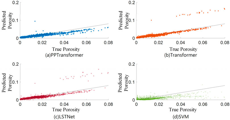
Figure 10. Cross plot porosity results from different methods on dataset III. (A-D) represent PPTransformer, Transformer, LSTNet, SVM, respectively.
3.5 PPTransformer for adding geologic constraints
From a geological perspective, the lithology of reservoir rocks exhibits stratal characteristics, mainly depending on their depositional environment and diagenetic processes. The depositional environment is closely related to lithological properties and can provide geological constraints. Porosity is closely associated with reservoir lithology, and lithology can provide geological constraints for porosity prediction. Therefore, we add lithological information (lithology curve) to the input curves to assist model training.
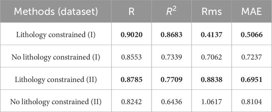
Figures 11, 12 show the predicted porosity of test datasets I and II, respectively. They show that the PPTransformer model predicts the trend of porosity curves. Visually, it is impossible to distinguish the improvement brought by adding lithology constraints. Table 5 presents different performance metrics of the test datasets. In datasets I and II, all four evaluation metrics show varying improvement degree after incorporating lithology constraints. It demonstrates that adding lithology constraints will enhance the accuracy of porosity prediction. Specifically, lithology-constrained porosity prediction exhibits a small disturbance for the type I and II reservoirs. However, dense limestone (red) and compact rock (yellow) do not significantly improve the porosity prediction accuracy. Therefore, further investigation on the lithology effect needs to be done.
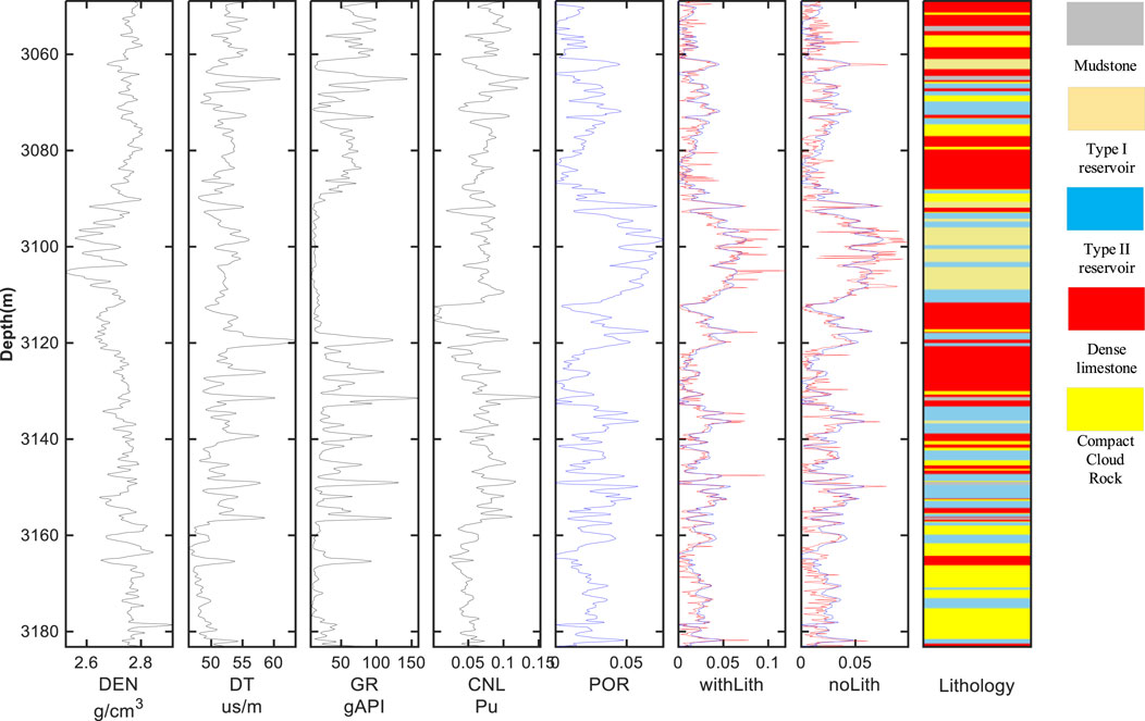
Figure 11. Porosity prediction results of well D, the blue curve is the label porosity, the red curve is the predicted porosity.
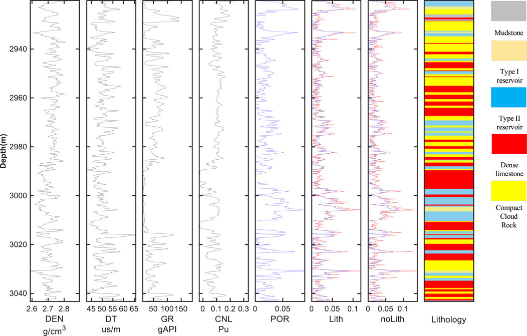
Figure 12. Porosity prediction results of well E, the blue curve is the label porosity, the red curve is the predicted porosity.
4 Conclusion
The PPTransformer network is developed to intelligently predict porosity in deep carbonate formations using AC, CGR, CNL, DEN, and RT as inputs. The PPTransformer network can simultaneously extract global and local features through a unique framework design. Results from the test dataset demonstrate that the proposed PPTransformer model is the most robust network. It can efficiently and accurately establish the nonlinear mapping relationship between input well logging data and porosity, outperforming the evaluation metrics of Transformer, LSTNet, and SVM models. Additionally, by incorporating lithology information into the model training process, the PPTransformer network will predict porosity more accurately.
Data availability statement
The original contributions presented in the study are included in the article/supplementary material, further inquiries can be directed to the corresponding author.
Author contributions
KH: Writing–original draft, Writing–review and editing. SC: Writing–original draft, Writing–review and editing. HK: Writing–original draft, Writing–review and editing. SY: Writing–original draft, Writing–review and editing. LZ: Writing–original draft, Writing–review and editing. YC: Writing–original draft, Writing–review and editing. XZ: Writing–original draft, Writing–review and editing. LZ: Writing–original draft, Writing–review and editing. HL: Writing–original draft, Writing–review and editing.
Funding
The author(s) declare that no financial support was received for the research, authorship, and/or publication of this article.
Conflict of interest
Authors KH, SC, HK, SY, LZ, YC were employed by China National Logging Corporation.
The remaining authors declare that the research was conducted in the absence of any commercial or financial relationships that could be construed as a potential conflict of interest.
Generative AI statement
The author(s) declare that no Generative AI was used in the creation of this manuscript.
Publisher’s note
All claims expressed in this article are solely those of the authors and do not necessarily represent those of their affiliated organizations, or those of the publisher, the editors and the reviewers. Any product that may be evaluated in this article, or claim that may be made by its manufacturer, is not guaranteed or endorsed by the publisher.
Supplementary material
The Supplementary Material for this article can be found online at: https://www.frontiersin.org/articles/10.3389/feart.2024.1510138/full#supplementary-material
References
An, P., and Cao, D. P. (2018). Research and application of deep learning-based lithology recognition method for logging. Adv. Geophys. 33 (3), 1029–1034. doi:10.6038/pg2018BB0319
Ao, Y. L., Li, H. Q., Zhu, L. P., Ali, S., and Yang, Z. G. (2019). The linear random forest algorithm and its advantages in machine learning assisted logging regression modeling. J. Petroleum Sci. Eng. 174, 776–789. doi:10.1016/j.petrol.2018.11.067
Bengio, Y., Simard, P., and Frasconi, P. (1994). Learning long-term dependencies with gradient descent is difficult. IEEE Trans. neural Netw. 5, 157–166. doi:10.1109/72.279181
Chen, W., Yang, L. Q., Zha, B., Zhang, M., and Chen, Y. K. (2020). Deep learning reservoir porosity prediction based on multilayer long short-term memory network. Geophysics 85 (4), WA213–WA225. doi:10.1190/geo2019-0261.1
Chen, Y., Zhao, L., Pan, J., Li, C., Xu, M., Li, K., et al. (2021). Deep carbonate reservoir characterisation using multi-seismic attributes via machine learning with physical constraints. J. Geophys. Eng. 18 (5), 761–775. doi:10.1093/jge/gxab049
Chen, Y. K., Saad, O. M., Savvaidis, A., Chen, Y. F., and Fomel, S. (2022). 3D microseismic monitoring using machine learning. J. Geophys. Res. Solid Earth 127 (3), e2021JB023842. doi:10.1029/2021JB023842
Chen, Y. K., Zhang, G. Y., Bai, M., Zu, S. H., Guan, Z., and Zhang, M. (2019). Automatic waveform classification and arrival picking based on convolutional neural network. Earth Space Sci. 6 (7), 1244–1261. doi:10.1029/2018EA000466
Fan, Y. R., Zhu, X. J., Deng, S. G., and Si, Z. W. (2012). Study on lithology identification technique of volcanic rocks in Nanbao No.5 tectonic structure. Adv. Geophys. 27 (4), 1. doi:10.6038/j.issn.1004-2903.2012.04.042
Feng, R. H., Mejer Hansen, T., Grana, D., and Balling, N. (2020). An unsupervised deep-learning method for porosity estimation based on poststack seismic data. Geophysics 85 (6), M97–M105. doi:10.1190/geo2020-0121.1
Fu, G. M., Yan, J. Y., Zhang, K., Hu, H., and Luo, F. (2017). Current status and progress of lithology identification technology. Prog. Geophys. 32 (1), 26–40. doi:10.6038/pg20170104
Hinton, G. E., and Salakhutdinov, R. R. (2006). Reducing the dimensionality of data with neural networks. science 313 (5786), 504–507. doi:10.1126/science.1127647
Hochreiter, S., and Schmidhuber, J. (1997). Long short-term memory. Neural Comput. 9, 1735–1780. doi:10.1162/neco.1997.9.8.1735
Ju, W., Han, X. H., Zhi, L. F., Fei, H. T., and Li, F. B. (2012). Application of Bayes stepwise discriminant analysis to identify the lithology of Es4 reservoir in Xin176 block. Comput. Technol. Phys. Chem. Explor. 34 (5), 576–581. doi:10.3969/j.issn.1001-1749.2012.05.14
Kalchbrenner, N., Danihelka, I., and Graves, A. (2015). Grid long short-term memory. arXiv preprint arXiv:1507.01526.
Karimpouli, S., Fathianpour, N., and Roohi, J. (2010). A new approach to improve neural networks algorithm in permeability prediction of petroleum reservoirs using supervised committee machine neural network (SCMNN). J. Petroleum Sci. Eng. 73 (3-4), 227–232. doi:10.1016/j.petrol.2010.07.003
Kazei, V., Ovcharenko, O., Plotnitskii, P., Peter, D., Zhang, X. L., and Alkhalifah, T. (2021). Mapping full seismic waveforms to vertical velocity profiles by deep learning. Geophysics 86 (5), R711–R721. doi:10.1190/geo2019-0473.1
Kumar, T., Seelam, N. K., and Rao, G. S. (2022). Lithology prediction from well log data using machine learning techniques: a case study from Talcher coalfield, Eastern India. J. Appl. Geophys. 199, 104605. doi:10.1016/j.jappgeo.2022.104605
Li, C., Shen, A. J., Chang, S. Y., Liang, Z. Z., Li, Z. L., and Meng, H. (2021). Application and comparison of machine learning method in carbonate rock facies logging identification example of Longwangmiao Formation stratigraphy in MX area, Sichuan Basin. Reserv. Eval. Dev. 11 (4), 586–596. doi:10.13809/j.cnki.cn32-1825/te.2021.04.015
Li, K. W., Xi, Y. J., Su, Z. X., Zhu, J. B., and Wang, B. S. (2021). Research on reservoir lithology prediction method based on convolutional recurrent neural network. Comput. Electr. Eng. 95, 107404. doi:10.1016/j.compeleceng.2021.107404
Li, W. C., Yao, G. Q., Huang, Y. T., and Ju, Z. L. (2012). Research on lithology identification method for logging low resistance oil formation in Wenchang 13-1 oilfield. J. Oil Gas 34 (12), 5. doi:10.3969/j.issn.1000-9752.2012.12.018
Lian, Z. Z., Tan, C. C., and Deng, K. C. (2013). Fuzzy pattern recognition based closeness method to discriminate the lithology of coalfield logging. Logging Technol. 37 (3), 4. doi:10.3969/j.issn.1004-1338.2013.03.013
Luo, H., Lai, F. Q., Dong, Z., and Xia, W. X. (2018). A lithology identification method for continental shale oil reservoir based on BP neural network. J. Geophys. Eng. 15 (3), 895–908. doi:10.1088/1742-2140/aaa4db
Luo, Z. R., Zhou, Y., Li, Y. X., Guo, L., Tuo, J. J., and Xia, X. L. (2021). Intelligent identification method of sedimentary microfacies based on DMC-BiLSTM. Pet. Phys. Explor. 61 (2), 253–261. doi:10.20944/preprints202103.0459.v1
Ma, L. F., Xiao, H. M., Tao, J. W., Zhang, F., Luo, Y. C., and Zhang, H. Q. (2022). Research and application of deep learning-based lithology classification. Sci. Technol. Eng. 22 (7), 2609–2617.
Mathew Nkurlu, B., Shen, C. B., Asante-Okyere, S., Mulashani, A. K., Chungu, J., and Wang, L. (2020). Prediction of permeability using group method of data handling (GMDH) neural network from well log data. Energies 13 (3), 551. doi:10.3390/en13030551
Mou, D., Wang, Z. W., Huang, Y. L., Xu, S., and Zhou, D. P. (2015). Identification of volcanic lithology based on SVM logging data-an example from the eastern depression of the Liaohe Basin. Geophys. J. 58 (5), 1785–1793. doi:10.6038/cjg20150528
Munchmeyer, J., Bindi, D., Leser, U., and Tilmann, F. (2021). The transformer earthquake alerting model: a new versatile approach to earthquake early warning. Geophys. J. Int. 225 (1), 646–656. doi:10.1093/gji/ggaa609
Pham, N., and Fomel, S. (2021). Uncertainty and interpretability analysis of encoder-decoder architecture for channel detection. Geophysics 86 (4), O49–O58. doi:10.1190/geo2020-0409.1
Ren, X. X., Hou, J. G., Song, S. H., Liu, Y. M., Chen, D. P., Wang, X. X., et al. (2019). Lithology identification using well logs: a method by integrating artificial neural networks and sedimentary patterns. J. Petroleum Sci. Eng. 182, 106336. doi:10.1016/j.petrol.2019.106336
Richardson, A. (2018). Seismic full-waveform inversion using deep learning tools and techniques. arXiv preprint arXiv:1801.07232.
Tian, Y., Sun, J. M., Wang, X., and Tian, G. D. (2010). Identification of reservoir lithology using stepwise method and Fisher's discriminant. Adv. Explor. Geophys. 33 (2), 126–129.
Vaswani, A. (2017). Attention is all you need. Adv. Neural Inf. Process. Syst. doi:10.5555/3295222.3295349
Wang, J., Cao, J. X., Liu, Z. Q., Zhou, X., and Lei, X. (2020). A prediction method of pre-drilling logging curve based on long and short-term memory network. J. Chengdu Univ. Technol. Nat. Sci. Ed. 47 (2), 227–236. CNKI:SUN:CDLG.0.2020-02-011.
Wang, Z. H., Zhu, X. M., Sun, Z. C., Luo, X. P., Dai, X. J., and Dai, Y. (2015). Logging data for igneous rock lithology identification and petrographic delineation in basins: a case study of Junggar Basin. Geol. Front. 22 (3), 15. doi:10.13745/j.esf.2015.03.022
Wu, J. L., Yin, X. L., and Xiao, H. (2018). Seeing permeability from images: fast prediction with convolutional neural networks. Sci. Bull. 63 (18), 1215–1222. doi:10.1016/j.scib.2018.08.006
Wu, Y., Schuster, M., Chen, Z., Le, Q. V., Norouzi, M., Macherey, W., et al. (2016). Google's neural machine translation system: bridging the gap between human and machine translation. arXiv Prepr. arXiv:1609.08144.
Wu, Z. Y., Zhang, X., Zhang, C. L., and Wang, H. Y. (2021). A lithology identification method based on LSTM recurrent neural network. Lithol. Reserv. 33 (3), 120–128. doi:10.12108/yxyqc.20210312
Xi, D. Y., and Zhang, T. (1995). Application of BP artificial neural network model in automatic identification of petrographic phase of logging data. Comput. Technol. Phys. Chem. Explor. 17 (1), 42–48.
Xiong, X. C., Cao, J. X., and Zhou, P. (2021). A petrographic prediction method based on bidirectional long and short-term memory neural networks. J. Chengdu Univ. Technol. Nat. Sci. Ed. 48 (2), 226–234. doi:10.3969/j.issn.1671-9727.2021.02.10
Yang, L. Q., Wang, S. D., Chen, X. H., Saad, O. M., Chen, W., Oboue, Y. A. S. I., et al. (2021). Unsupervised 3-D random noise attenuation using deep skip autoencoder. IEEE Trans. Geoscience Remote Sens. 60, 1–16. doi:10.1109/TGRS.2021.3100455
Zhang, D. X., Chen, Y. T., and Meng, J. (2018). A method for logging curve generation based on recurrent neural network. Petroleum Explor. Dev. 45 (4), 598–607. CNKI:SUN:SKYK.0.2018-04-007.
Zhang, G. Y., Wang, Z. Z., and Chen, Y. K. (2018). Deep learning for seismic lithology prediction. Geophys. J. Int. 215 (2), 1368–1387. doi:10.1093/gji/ggy344
Zhang, G. Y., Wang, Z. Z., Mohaghegh, S., Lin, C. Y., Sun, Y. A., and Pei, S. J. (2021). Pattern visualization and understanding of machine learning models for permeability prediction in tight sandstone reservoirs. J. Petroleum Sci. Eng. 200, 108142. doi:10.1016/j.petrol.2020.108142
Zheng, J., Lu, J. R., Peng, S. P., and Jiang, T. Q. (2017). An automatic microseismic or acoustic emission arrival identification scheme with deep recurrent neural networks. Geophys. J. Int. 212, 1389–1397. doi:10.1093/gji/ggx487
Keywords: deep carbonate rocks, porosity prediction, PPTransformer, logging curves, deep learning
Citation: Huang K, Cui S, Kan H, Yang S, Zhang L, Chen Y, Zhang X, Zhu L and Li H (2024) Porosity identification using residual PPTransformer network. Front. Earth Sci. 12:1510138. doi: 10.3389/feart.2024.1510138
Received: 12 October 2024; Accepted: 04 December 2024;
Published: 18 December 2024.
Edited by:
Xingye Liu, Chengdu University of Technology, ChinaReviewed by:
Qingzhi Hou, Tianjin University, ChinaLuanxiao Zhao, Tongji University, China
Ziqi Jin, Northeast Petroleum University, China
Copyright © 2024 Huang, Cui, Kan, Yang, Zhang, Chen, Zhang, Zhu and Li. This is an open-access article distributed under the terms of the Creative Commons Attribution License (CC BY). The use, distribution or reproduction in other forums is permitted, provided the original author(s) and the copyright owner(s) are credited and that the original publication in this journal is cited, in accordance with accepted academic practice. No use, distribution or reproduction is permitted which does not comply with these terms.
*Correspondence: Huaiyuan Li, bGlodWFpeTIwMDFAc3R1LnhqdHUuZWR1LmNu
 Ke Huang1
 Huaiyuan Li
