Wavefield-reconstruction-based full waveform inversion on noisy data in seismic exploration

Full waveform inversion (FWI) is commonly used in seismic exploration to calculate parameters of the medium, such as velocity, from the signal as it passes through the medium. To obtain an accurate result, FWI usually needs to have an initial model that is not too far from the true velocity model. However, using noisy low-frequency data to build the initial model can be a challenge for FWI in practice. To solve this problem, we propose a wavefield reconstruction method based on the first type of Rayleigh–Sommerfeld integral and apply the multiple reconstructed wavefield (MRW) to the gradient calculation. The MRW combines different reconstructed wavefields, and those wavefield components with similar properties are enhanced by superposition. The reflected waves, which are critical for updating the deep portions of the velocity model, are strengthened in the MRW to significantly reduce the negative effects of data noise when calculating FWI gradients. The MRW optimizes the gradient of the FWI, yielding high-quality results despite noise interference. Incorporating the MRW into the FWI effectively mitigates overfitting problems associated with noisy data and improves the robustness of the FWI.

1 Introduction

Full waveform inversion (FWI) is a powerful technique used in seismic exploration to obtain high-resolution images of subsurface structures. Since it is proposed by Lailly (1983) and Tarantola (1984), many researchers are trying to use FWI to solve practical inverse problems. However, FWI has some shortcomings preventing it from being used in some practices. One of the key points is that FWI is a nonlinear inverse problem and local minima in the objective function make it difficult for FWI to obtain ideal results. Multiscale inversion strategies are developed to reduce this nonlinearity. The inversion scheme from low to high frequency (Pratt and Worthington, 1990; Sirgue and Pratt, 2004; Xie et al., 2024) reduces the influence of local minimum on the global convergence of inversion. Shin and Ha (2008) found that the Laplace-domain inversion can more easily obtain a smooth background velocity model than the frequency-domain inversion and the frequency-domain inversion whose initial model is the result of the Laplace-domain inversion can successfully invert complex models. Brossier et al. (2009a) tested some multiscale strategies of elastic FWI in the frequency domain, and they thought that the inversion strategy with frequency group data as input has less cycle-skipping phenomena than that with single frequency data as input. In the time domain, the multiscale FWI decomposes the data into different frequency parts, and the inversion processes the different parts of the data in order of frequency from low to high (Bunks et al., 1995). With the existing computing capacity, Vigh and Starr (2008) realized the 3D multiscale FWI in time domain by using the plane-wave gathers as input. Poncet et al. (2018) and Smith et al. (2019) successfully applied 3D FWI to the actual acquisition data and obtained accurate results. Another way to solve the nonlinearity was proposed by Choi and Alkhalifah (2012), Alkhalifah and Choi (2012), and they took advantage of the unwrapped phase to construct the objective function, so that the waveform inversion can avoid cycle-skipping.

Some researchers (Mora, 1987; 1988; Pratt et al., 1996) had emphasized that it is a key point for the common use of FWI in practice to recover large-scale structures from long-offset data. Vigh et al. (2013) introduced a comprehensive two-coil multi-ship acquisition methodology, which has been demonstrated to be an effective approach for capturing long-offset oceanic 3D seismic data. da Silva et al. (2024) presented a novel circular acquisition geometry for use in the ocean, which facilitates ultra-long offset acquisition while simultaneously reducing costs. Although long-offset data are critical to improving FWI results, they are not always available (Virieux and Operto, 2009). Wu et al. (2013), Wu et al. (2014) proposed an envelope inversion, which extracts ultra-low-frequency information from seismic records, to provide a smooth initial model for the time-domain multiscale FWI. Alkhalifah and Wu (2016) revealed that applying the multi-scattering wavefield to inversion helped to obtain a smooth background model. In the short-offset acquisition system, due to the limited penetration depth of the turning and refracted waves, only the reflected wave in the data carries the information of the deep part of the model (Yao et al., 2020). In reality, the data usually contain a lot of noise, which makes the data quality quite low. The presence of noise can result in the amplitude of the data becoming anomalous, thereby impeding the inversion model from approximating the true model (Asnaashari et al., 2013; Virieux and Operto, 2009). The L₂ criterion will amplify the negative effects of the noise, resulting in inversion failure, if the data residuals are caused by non-Gaussian noise (Brossier et al., 2009b). Constable (1988) discussed the problem of parameter estimation in non-Gaussian noise and evaluated various parameter estimation algorithms. Mitigating the effects of data amplitude errors is one of the challenges for FWI (Virieux and Operto, 2009). Generally, low-frequency data generated by active sources are more likely to be corrupted by noise. The minimum frequency of the filtered data tends to be greater than 3 Hz (Tejero et al., 2015), which is not sufficient to meet the requirement of the FWI for a low frequency signal. Adding regularization term to the objective function is one of the commonly used methods to resist noise. Brossier et al. (2009b), Brossier et al. (2010) provided evidence that the L₁ norm of the data residual remains relatively unaffected by non-Gaussian noise. Additionally, the results indicated that the elastic frequency-domain FWI, which employs an objective function based on the L₁ norm, is robust. As a consequence of the non-differentiability of the L₁-regularized objective function, the limited memory quasi-Newton method (l-BFGS) (Byrd et al., 1994) is not suitable for combination with L₁-regularization (Andrew and Gao, 2007; Dai et al., 2017). Andrew and Gao (2007) proposed the Orthant-wise Limited Memory Quasi-Newton method, which can be combined with L₁-regularization, based on l-BFGS. Dai et al. (2017) applied noisy data in FWI with a mix of the Orthant-wise Limited Memory Quasi-Newton method and L₁-regularization, and their method showed acceptable resistance to noise. Cui et al. (2017) combined reflection full waveform inversion and FWI to obtain relatively accurate deep structures, and this method has some robustness to noise. Wang et al. (2021) successfully used machine learning model with good noise immunity to predict velocity model from synthetic data and recorded field data. da Silva and Kaniadakis (2022) improved FWI by building an optimal transport metric based on κ-statistics to enable it to better handle outliers in the data.

In the field of imaging, Berryhill (1979) proposed wave equation datuming to solve the problem of seismic data profile distortion caused by the complexity of the model. The survey sinking (Claerbout, 1985; Wu et al., 2017) was proposed to extrapolate and rebuild the seismic wavefield in depth. Chen and Jia (2014) proposed a staining algorithm marking part of the extrapolated wavefield to improve the imaging resolution of the target region. Based on this, Li and Jia (2017) developed a generalized staining algorithm in the time domain, which enhanced the resolution of weakly illuminated areas while preserving the imaging amplitude. According to the concept of the generalized staining algorithm, Yu and Jia (2021) used the first type of Rayleigh–Sommerfeld (RS) integral (Berkhout, 1984) to adjust the composition of the wavefield.

In this study, we develop an algorithm of multiple wavefield reconstruction and illustrate the implementation of the algorithm for l-BFGS inversion (Byrd et al., 1994) in the frequency domain. The totally reflected wavefield is generated along with the reconstructed wavefield. Reflected waves are very important for the inversion of the deep parts of the velocity model. The superposition of the reconstructed wavefield enhances the reflected waves, suppresses the invalid waves and yields multiple reconstructed wavefield (MRW). We utilize the MRW to optimize the gradient of FWI to improve the robustness of the FWI with noisy data. In addition, we analyze computational efficiency of the FWI using the MRW under strong Wolfe conditions (Nocedal and Wright, 1999).

2 Materials and methods

2.1 Frequency-domain reconstructed wavefield

The two-dimensional acoustic equation in the frequency domain has the general form of

$\left(\frac{{\partial }^2}{\partial x^2}+\frac{{\partial }^2}{\partial z^2}+\frac{{\omega }^2}{{v\left(x,z\right)}^2}\right)a\left(x,z,\omega \right)=s\left(x,z,\omega \right),(1)$

where ω is the angular frequency, v is the P-wave velocity, a is the pressure field, s represents the seismic source, and x and z represent the horizontal and vertical coordinates, respectively. The matrix equation with seismic source related to Equation 1 is given by

$\mathbf{F}\mathbf{A}=\mathbf{S},(2)$

where F represents the Helmholtz operator matrix, A is the pressure field matrix, and S is the source matrix. The LU factorization techniques are generally used to solve Equation 2 by

$\mathbf{F}=\mathbf{L}\mathbf{U},(3)$

$\mathbf{Y}={\mathbf{L}}^{-1}\mathbf{S},(4)$

$\mathbf{A}={\mathbf{U}}^{-1}\mathbf{Y}.(5)$

We can simply express Equation 2 as

$\mathbf{A}={\mathbf{F}}^{-1}\mathbf{S}.(6)$

As illustrated in Figure 1, according to the frequency-domain Kirchhoff integral (Berkhout, 1984), the wavefield at a point (P₁) situated outside of the closed surface O can be expressed as

$a\left(P_1,\omega \right)=-\frac{1}{4\mathrm{\pi }}\underset{\mathbf{O}}{\iint }\left[\left(\frac{\partial a}{\partial \mathbf{n}}+\mathrm{j}k\frac{\partial {\mathit{r}}_1}{\partial \mathbf{n}}a+\frac{1}{r_1}\frac{\partial {\mathit{r}}_1}{\partial \mathbf{n}}a\right)G\right]\mathrm{d}O,(7)$

where G is Green’s function related to r₁ or r₂, k = ω/v and j is the imaginary unit. In this equation, the variable “a” on the right-hand side represents the wavefield on the closed surface O. We can calculate wavefields at other spatial locations based on the known wavefields on the closed surface O and their directional derivatives. The wavefield at a point (P₂) within the closed surface O can be expressed as

$a\left(P_2,\omega \right)=\underset{\mathbf{\Omega }}{\iiint }s\left(\omega \right)G\mathrm{d}\mathrm{\Omega }+\frac{1}{4\mathrm{\pi }}\underset{\mathbf{O}}{\iint }\left[\left(\frac{\partial a}{\partial \mathbf{n}}+\mathrm{j}k\frac{\partial {\mathit{r}}_2}{\partial \mathbf{n}}a+\frac{1}{r_2}\frac{\partial {\mathit{r}}_2}{\partial \mathbf{n}}a\right)G\right]\mathrm{d}O.(8)$

Figure 1

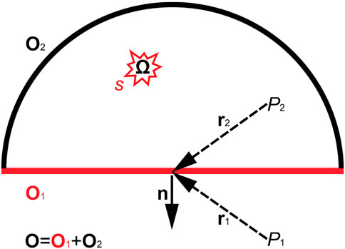
Figure 1. Schematic diagram of the Kirchhoff integral. O is the closed surface consisting of O₁ and O₂; n is the outer normal direction of O; P₁ and P₂ are two typical space locations; r₁ and r₂ are the vectors from P₁ and P₂ to a point on O, respectively; the source s is located in the volume Ω.

The volume integral term represents the contribution of the source distributed in the volume Ω to the wavefield at P₂. The first term of the equation can be regarded as the background wavefield, and the second term is the primary or multiple scattering wavefield. If O is infinite, the energy on it has little influence for the wavefield. Therefore, we can ignore the second term of Equation 8 and then

$a\left(P_2,\omega \right)=\underset{\mathbf{\Omega }}{\iiint }s\left(\omega \right)G\mathrm{d}\mathrm{\Omega }.(9)$

Comparing Equation 9 with Equation 6, we have Equation 10 as

${\mathbf{F}}^{-1}=\underset{\mathbf{\Omega }}{\iiint }G\mathrm{d}\mathrm{\Omega }.(10)$

When subjected to rigid boundary conditions, the Kirchhoff integral, as illustrated in Equation 7, can be reduced to the first type of RS integral (Berkhout, 1984)

$a\left(P_1,\omega \right)=-\frac{1}{2\mathrm{\pi }}\underset{{\mathbf{O}}_1}{\iint }\left[\left(\frac{\partial a}{\partial \mathbf{n}}\right)G\right]\mathrm{d}O.(11)$

This equation demonstrates that the wavefield at P₁ can be calculated using the wavefields on the plane O₁ and their directional derivative. Huygens’ principle (Born and Wolf, 1999) states that fluctuations on the surface O₁ can be treated as sources, thereby allowing $\mathrm{\partial }a/\mathrm{\partial }\mathbf{n}$ in Equation 11 to be treated as a source. ${\iiint }_{\mathbf{\Omega }}G\mathrm{d}\mathrm{\Omega }$ and ${\iint }_{{\mathbf{O}}_1}G\mathrm{d}O$ represent the same wave propagator ${\mathbf{F}}^{-1}$ for a given velocity model. In Equation 6, A represents the wavefield for the entire space. In Equation 11, $a\left(P_1,\omega \right)$ is the wavefield at P₁. Accordingly, Equation 11 can be expressed in the following form:

$\mathbf{A}={\beta \mathbf{F}}^{-1}\mathbf{E},(12)$

where A is the reconstructed wavefield, β represents the amplitude, E acts as the reconstructed source, and

$E=\frac{\partial a}{\partial \mathbf{n}}.(13)$

Where E represents an element of E. Equation 12 is the frequency-domain formula of wavefield reconstruction. As shown in Figure 2, the red lines represent the positions of the reconstructed sources (E₁-E_n) and the blue areas represent where the reconstructed wavefields propagate. According to the first type of RS integral (Berkhout, 1984), the wavefields propagating in the white areas above the reconstructed sources are total reflections of the reconstructed wavefields from the reconstructed sources. Unless otherwise specified, the reconstructed wavefield mentioned in the following section of this paper refers to the wavefield below the reconstructed source. After obtaining the original wavefield, we use the original wavefield on the red line to calculate the reconstructed source (such as E₁) according to Equation 13. Subsequently, the reconstructed source (such as E₁) is positioned in the corresponding red line position, thereby yielding the reconstructed wavefield (such as C₁) in accordance with Equation 12. For simplicity, we set a constant on β to calculate the reconstructed wavefield. The reconstructed source can be placed at any desired location, and different reconstructed wavefields (such as C₁–C_n) can be generated by loading the appropriate reconstructed sources (such as E₁–E_n).

Figure 2

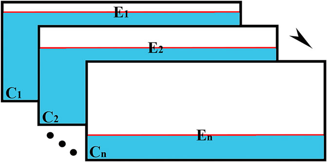
Figure 2. Schematic diagram of multiple wavefield reconstruction. The red lines represent the positions of the reconstructed sources (E₁-E_n); the blue areas represent where the reconstructed wavefields (C₁-C_n) propagate; the wavefields propagating in the white areas above the reconstructed sources are total reflections of the reconstructed wavefields from the reconstructed sources.

2.2 Frequency-domain FWI utilizing MRW

For a two-dimensional velocity model as shown in Figure 2, the reconstructed sources (E₁–E_n) calculated with the original wavefields at different depths are loaded to obtain reconstructed wavefields (C₁–C_n). We sum a proportion of the reconstructed wavefields to obtain the MRW and enhance reflected waves in the MRW. If we load all the reconstructed sources to a model at the same time, according to Equation 12, we have (Yu and Jia, 2021)

$\mathbf{C}={\beta \mathbf{F}}^{-1}\left({\mathbf{E}}_1+{\mathbf{E}}_2+···+{\mathbf{E}}_{\mathrm{n}}\right)={\mathbf{C}}_1+{\mathbf{C}}_2+···+{\mathbf{C}}_{\mathrm{n}}.(14)$

The wavefield calculated by Equation 14 is the MRW. According to Figure 2 and Equation 14, The different depth parts of the MRW are the superposition of different amounts of the reconstructed wavefield. For amplitude preservation, the different depth parts of the MRW should be divided by the number of stacking times. The value of n can be freely set according to the specific needs and the size of the velocity model. The reflected waves in the MRW, which can facilitate the update of the deep velocity (Lian et al., 2018; Dong et al., 2018; Yao et al., 2020), are enhanced. The MRW is used in place of the original wavefield to optimize the gradient of the FWI. For noisy data, dot product of the adjoint wavefield with the MRW can mitigate the effect of noise on FWI gradients.

The FWI problem is to minimize the objective function

$\min f\left(\mathit{q}\right)=\frac{1}{2}{\displaystyle \sum _{\omega }}{\displaystyle \sum _i}{‖{\mathbf{R}}_i{\mathbf{A}}_i-{\mathbf{B}}_i‖}^2,(15)$

where q is the squared slowness, B_i denotes the recorded data, R_i represents the operator for extracting simulated data from simulated wavefield A_i, and the subscript i indicates the shot-gather number. The gradient of the objective function (Equation 15) is expressed by the adjoint state method (Plessix, 2006; Métivier et al., 2012) as

$\nabla f=Re\left({\displaystyle \sum _{\omega }}{\displaystyle \sum _i}{\omega }^2{\mathbf{\lambda }}_i^{*}\left(\omega \right){\mathbf{A}}_i\left(\omega \right)\right),(16)$

where λ_i^* is the complex conjugation of the adjoint wavefield, and Re denotes the real part of a complex value. According to Taylor series, the exact model update format is

${\mathbf{Q}}^{l+1}={\mathbf{Q}}^l-{\mathbf{H}}^{-1\left(l\right)}{\nabla f}^l,(17)$

where l represents the number of updates, Q and H are the parameter matrix and the Hessian matrix, respectively. Using l-BFGS method, we approximate the Hessian matrix from Equation 17 to derive Equation 18, which is

${\mathbf{Q}}^{l+1}={\mathbf{Q}}^l+{\alpha }^l{\mathbf{D}}^l,(18)$

where α denotes the step length, and D is the search direction. In this paper, the line search method for calculating the step length satisfies the strong Wolfe conditions (Nocedal and Wright, 1999)

$f\left({\mathbf{Q}}^l+{\alpha }^p{\mathbf{D}}^l\right)\le f\left({\mathbf{Q}}^l\right)+{\theta }_1{\alpha }^p{\nabla f}_l^T{\mathbf{D}}^l,(19)$

and

$\left|{\nabla f\left({\mathbf{Q}}^l+{\alpha }^p{\mathbf{D}}^l\right)}^T{\mathbf{D}}^l\right|\le {\theta }_2\left|{\nabla f}_l^T{\mathbf{D}}^l\right|,(20)$

where 0 < θ₁ < θ₂ < 1, T denotes the matrix transpose, and p represents the p-th searching iteration.

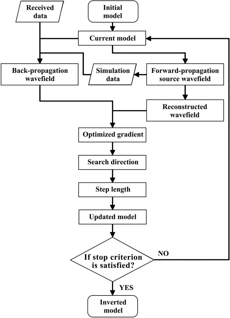
We used the l-BFGS to explain the FWI utilizing the MRW (i.e., l-BFGS-MRW). In the process of the l-BFGS-MRW inversion, after the original wavefield (Equation 6) of forward propagation is obtained, the MRW is calculated according to Equation 14 and then applied to the optimized gradient by Equation 16. The forward wavefield A_i(ω) in Equation 16 is replaced by the MRW, and other processes are consistent with the original l-BFGS inversion. The specific details of the workflow of the l-BFGS-MRW inversion are shown in Figure 3.

Figure 3

Figure 3. The workflow of the l-BFGS-MRW.

In order to evaluate the inversion results quantitatively, we introduce the residual sum of squares (RSS), defined by Equation 21 as:

$\text{RSS}={{\displaystyle \sum _x}{\displaystyle \sum _z}\left[v\left(x,z\right)-v^{\text{true}}\left(x,z\right)\right]}^2,(21)$

where $v\left(x,z\right)$ and $v^{\text{true}}\left(x,z\right)$ represent inversion model and the true model respectively. The RSS represents the discrepancy between the inversion results and the true model. A smaller RSS value indicates a greater similarity between the inversion results and the true model.

3 Results

3.1 Numerical analysis on frequency-domain reconstructed wavefield

Figure 4A shows a two-layer velocity model, where the red hexagon represents the location of the seismic source. The solid magenta line denotes a part of a closed surface O with n as its outer normal vector. Note that the solid magenta line also represents the position of the reconstructed source E. The grid spacing was 15 m. Figure 4B shows the original wavefield for a frequency of 10 Hz. After obtaining the original wavefield, we calculated the reconstructed source and the reconstructed wavefield according to Equations 13 and 12, respectively. Figure 4C shows the reconstructed wavefield for 10 Hz, and the wavefield above the reconstructed source is the totally reflected wavefield. To reconstruct the wavefield accurately, the reconstructed source contained a number of grid points in the n-direction. The residual between the reconstructed wavefield and the original wavefield is displayed in Figure 4D. Although the residual wavefield has different spatial characteristics, the energies of all its components are much smaller than those of the original wavefield (Figure 4B). Figure 4E shows the real parts of the original wavefield and the reconstructed wavefield along the dotted white line in Figure 4A. As shown in Figure 4E, the curves of the original wavefield and the reconstructed wavefield are overlapped and their residual is approximately three orders of magnitude smaller than the original wavefield, which indicates that the reconstructed wavefield is almost equal to the original wavefield when their positions are close to the source. When the position of the reconstruction wavefield is far from the source, as shown in Figure 4F, there is a small amplitude difference between the reconstructed wavefield and the original wavefield. Because we just take attention to a part of the closed surface O and ignore the rest of it, some energy, which exist in the original wavefield, is not involved in the reconstruction wavefield; therefore, the reconstructed wavefield and the original wavefield have little amplitude difference in the area far from the source.

Figure 4

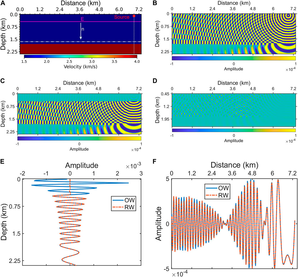
Figure 4. Two-layer velocity model and frequency-domain wavefield. (A) Two-layer velocity model; (B) original wavefield for 10 Hz; (C) reconstructed wavefield for 10 Hz; (D) the residual between the reconstructed wavefield and the original wavefield; (E) the real parts of the original wavefield (OW) and the reconstructed wavefield (RW) along the dotted white line in (A); (F) the real parts of the original wavefield and the reconstructed wavefield along the dashdotted white line in (A).

In the example of a complex model, we can get the same conclusion as the former. Figure 5A shows a slice of the Marmousi velocity model, where the solid magenta line represents the location of the reconstructed source. The shot was located at distance of 6.9 km and depth of 0.09 km. The grid spacing was 15 m. Figure 5B displays the original wavefield for 10 Hz, and Figure 5C displays the reconstructed wavefield for 10 Hz. The residual between the reconstructed wavefield and the original wavefield is shown in Figure 5D.

Figure 5

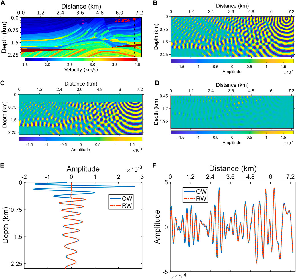
Figure 5. (A) A slice of the Marmousi velocity model; (B) original wavefield for 10 Hz; (C) reconstructed wavefield for 10 Hz; (D) the residual between the reconstructed wavefield and the original wavefield; (E) the real parts of the original wavefield and the reconstructed wavefield on the dotted black line in (A); (F) the real parts of the original wavefield and the reconstructed wavefield on the dashdotted black line in (A).

Figure 5E illustrates the real parts of the original wavefield and the reconstructed wavefield on the dotted black line in Figure 5A. The reconstructed wavefield in Figure 5E is close to the source; therefore, the residual of the two wavefields is approximately 2 orders of magnitude smaller than the original wavefield, which suggests that the two wavefields are almost the same. Figure 5F shows the real parts of the original wavefield and the reconstructed wavefield on the dashdotted black line in Figure 5A, which indicates that the two wavefields have amplitude differences in the area far from the source. Nevertheless, as Figure 5F indicates, the reconstructed wavefield still preserves most of the energy of the original wavefield and the phases of these two wavefields are almost identical.

In the reconstructed wavefield, most of the original wavefield are completely preserved. Although the reconstructed wavefield far from the source have small energy differences from the original wavefield, their phases are almost identical. These small differences are not enough to interfere with FWI to obtain accurate results. In addition, according to the propagation path of the deep residual wavefields (the deep parts of Figures 4D, 5D), lots of the residual wavefields propagated outside the study area and could not be detected by the geophones distributed on the surface; the deep energy that cannot be received by the geophones is useless for FWI. The MRW is a superposition of different reconstructed wavefields; in the MRW, the components of the wavefield with the same character, including those far from the source, are enhanced by superposition; among them, the reflected waves are more enhanced because they are reconstructed more accurately compared to the other components. In other words, the proportion of the reflected waves in energy is increased.

Updates to the deep part of the model rely primarily on reflected waves (Lian et al., 2018; Dong et al., 2018; Yao et al., 2020). Noise in the data can lead to unwanted adjoint wavefields; in the deep part of the model, the dot product of these unwanted adjoint wavefields with the deep wavefield components that are useless for the FWI gradient is detrimental. The enhanced reflected waves will be highlighted in the gradient calculation to suppress the detrimental dot product. Therefore, the MRW can be used to mitigate the adverse effects of data noise on the FWI gradient. In addition, the difference between the MRW and the original wavefield will avoid FWI from overfitting the noisy data. For these reasons, when we employ the MRW in FWI, we generally obtain a result with high resolution.

3.2 Experiments of frequency-domain reconstructed FWI

For the FWI experiments below, the source was a Ricker wavelet and the dominant frequency was 7 Hz. 436 geophones were evenly distributed on the surface and 109 seismic sources were sequentially placed on the surface. The grid spacing was 25 m and the time interval was 0.5 ms. The recorded data were generated by forward modeling with uniformly distributed noise added. Some of the data are displayed in Figure 6. We made J to represent the ratio of the mean value of the noise energy to the mean value of the signal energy. We took the model in Figure 7A as the true model and employed the initial model shown in Figure 7B. The initial model is derived by applying a high degree of smoothing to the true model. During the inversion (Figures 2, 3), the reconstructed sources (E₁−E_n) filled the entire current model space to obtain the MRW. Figures 7C, E, G illustrate the l-BFGS results (1–6 Hz) when J is 8.97%, 53.83%, 269.13%, respectively. Figures 7D, F, H show the l-BFGS-MRW results (1–6 Hz) when J is 8.97%, 53.83%, 269.13%, respectively.

Figure 6

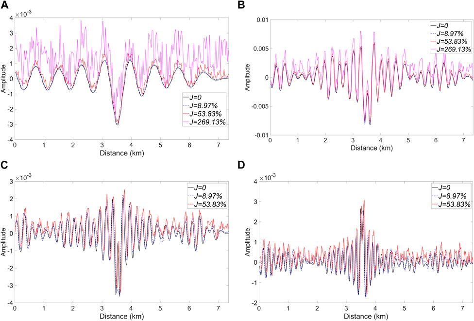
Figure 6. (A–D) display the frequency-domain data of 2, 6, 7 and 10 Hz, respectively; The source is a Ricker wavelet with a dominant frequency of 7 Hz; J represents the ratio of the mean value of the noise energy to the mean value of the signal energy.

Figure 7

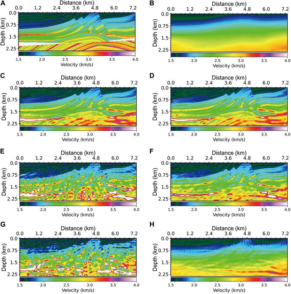
Figure 7. (A) shows a slice of the Marmousi velocity model and (B) is the initial velocity model for inversion. J represents the ratio of the mean value of the noise energy to the mean value of the signal energy. (C), (E) and (G) show the l-BFGS results (1–6 Hz) when J is 8.97%, 53.83%, 269.13%, respectively; (D), (F) and (H) show the l-BFGS-MRW results (1–6 Hz) when J is 8.97%, 53.83%, 269.13%, respectively.

In the experiment on data with a modest noise level (J = 8.97%), the results of l-BFGS-MRW and l-BFGS are not significantly different. The residual sum of squares (RSS) of the l-BFGS-MRW result is 1,689, which is slightly smaller than that (2,159) of the l-BFGS result. For a detailed comparison, Figure 8A exhibits the velocities extracted along a line (Distance = 0–7.335 km, Depth = 2 km) in Figures 7A, C, D. The result of l-BFGS-MRW is closer to the true model than that of l-BFGS and there are some large outliers in the l-BFGS result. When J is 53.83%, the RSS of the l-BFGS-MRW result shown in Figure 7F is 2,187, which is much smaller than that (29,533) of the l-BFGS result shown in Figure 7E. The result of l-BFGS-MRW has fewer artifacts and a clearer structure than that of l-BFGS. Figure 8B displays the velocities extracted along a line (Distance = 0–7.335 km, Depth = 1.85 km) in Figures 7A, E, F. The l-BFGS result has many large outliers and the l-BFGS-MRW result is much better than the l-BFGS result. The l-BFGS-MRW inversion is more robust than the l-BFGS inversion. Despite the high noise level, the l-BFGS-MRW inversion can obtain a relatively accurate initial model for high-frequency inversion. When J is large as 269.13%, the result of l-BFGS (Figure 7G) becomes worse than its former result. Because the data is severely damaged by noise, the l-BFGS-MRW inversion can only use less information from the data and restore the low-wavenumber velocity structure as demonstrated in Figure 7H. The RSS of l-BFGS-MRW result is 2,728, while that of l-BFGS result is 100,370.

Figure 8

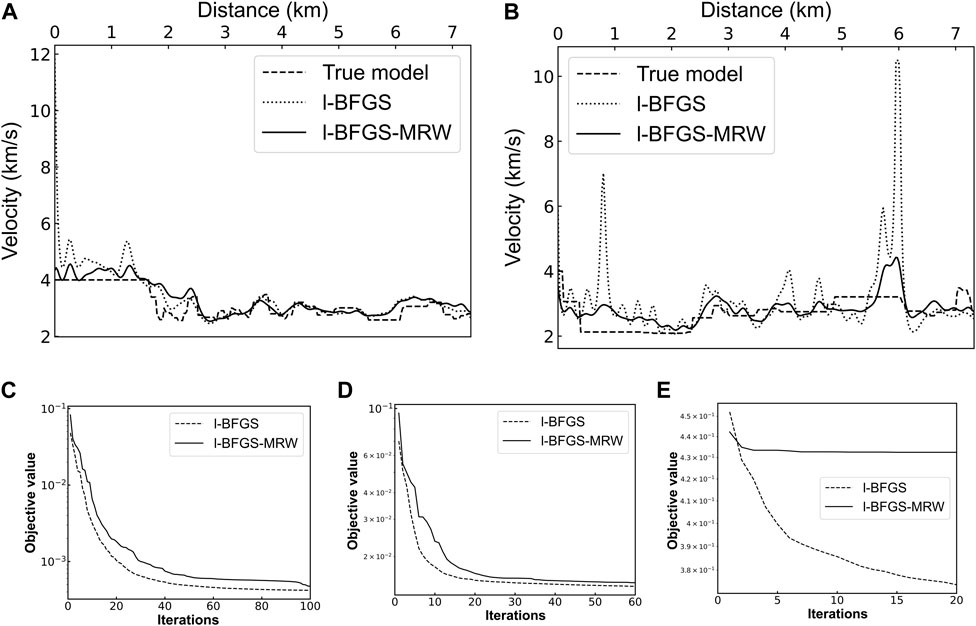
Figure 8. (A) The velocities extracted along a line (Distance = 0–7.335 km, Depth = 2 km) in Figures 7A, C, D; (B) the velocities extracted along a line (Distance = 0–7.335 km, Depth = 1.85 km) in Figures 7A, E, F; (C) the data convergence of 1–6 Hz inversion for Figures 7C, D; (D) the data convergence of 1–6 Hz inversion for Figures 7E, F; (E) the data convergence of 1–6 Hz inversion for Figures 7G, H.

The data convergence of the 1–6 Hz inversion corresponding to Figures 7C, D is exhibited in Figure 8C. Figure 8D shows the data convergence of the 1–6 Hz inversion corresponding to Figures 7E, F. The values of the objective function following the initial iteration are distinct, resulting in a misalignment of the curves at the starting point in both figures. As illustrated in Figures 8C, D, despite the disparate descending paths of the objective values for the two methods, all objective values converge to a sufficient degree with the same number of iterations. It is challenging to eliminate the introduction of data noise into the calculation of the objective value. While fitting data noise may reduce the objective value, it also carries the risk of diverging the inversion model from the true model. Because the gradients were optimized by the MRW, the models of the l-BFGS-MRW inversion would resist being updated in the direction of data noise guidance. On the contrary, the l-BFGS inversion would fall into local minima generated by data noise, which can result in inversion models that do not approximate the true model. As a consequence of the aforementioned factors, the objective values of l-BFGS-MRW inversion are larger than those of l-BFGS inversion after numerous iterations. Figure 8E illustrates the same phenomenon as the formers. When J equal to 269.13%, the value of the objective function that utilizes the strong noisy data is meaningless. Our gradient construction can hardly reduce the value of the objective function that utilizes the strong noisy data. Therefore, the objective value of the l-BFGS-MRW was not sufficiently reduced (Figure 8E). The l-BFGS inversion overfitting the recorded data is equivalent to fitting some data noise. Despite the objective values being reduced to relatively low values, the results shown in Figures 7E, G exhibit significant discrepancies from the actual models.

The grid spacing of the low-frequency inversion and the high-frequency inversion is 25 m and 15 m, respectively. RSS is calculated based on the velocity at the grid point and all RSS are kept as integers. The low-frequency inversion has a larger grid spacing and fewer grid points than the high-frequency inversion, so the RSS of the high-frequency inversion result may be larger than that of the low-frequency inversion result for the same inversion method. In the experiment of the 7–10 Hz inversion, Figure 9A demonstrates the l-BFGS result (J = 8.97%) with the initial model shown in Figures 7C, 9B illustrates the l-BFGS-MRW result (J = 8.97%) with the initial model shown in Figure 7D. The RSS of the l-BFGS-MRW result is 3,897, which is smaller than that (5,224) of the l-BFGS result. Although J is small, the l-BFGS result shown in Figure 9A has a low resolution in the deep part of the model. In contrast, the l-BFGS-MRW result has a high resolution in the entire model space. Figure 9C displays the l-BFGS result (J = 53.83%) with the initial model shown in Figures 7E, 9D exhibits the l-BFGS-MRW result (J = 53.83%) with the initial model shown in Figure 7F. Their RSS are 37,822 and 167,925 respectively. Although the noise level has increased, the result of l-BFGS-MRW still has a higher resolution than that of l-BFGS. The detailed comparisons for the results of the two methods are shown in Figures 10A, B. In order to facilitate the display, some extremely large outliers in the results of l-BFGS have been manually suppressed. In the high-frequency inversion with noisy data, the l-BFGS-MRW is still robust. The aforementioned RSS have been synthesized into Table 1 for purposes of clarity and ease of reference.

Figure 9

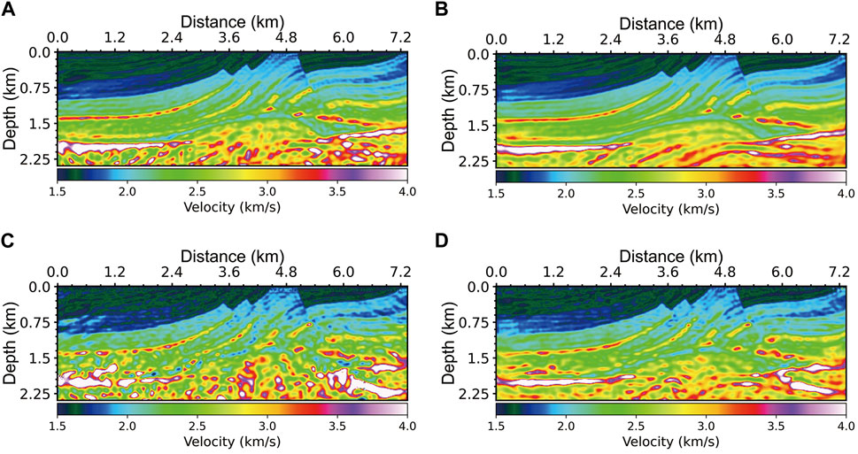
Figure 9. The inversion results (7–10 Hz) with different J. (A) The l-BFGS result (7–10 Hz, J = 8.97%) with the initial model shown in Figure 7C; (B) the l-BFGS-MRW result (7–10 Hz, J = 8.97%) with the initial model shown in Figure 7D; (C) the l-BFGS result (7–10 Hz, J = 53.83%) with the initial model shown in Figure 7E; (D) the l-BFGS-MRW result (7–10 Hz, J = 53.83%) with the initial model shown in Figure 7F.

Figure 10

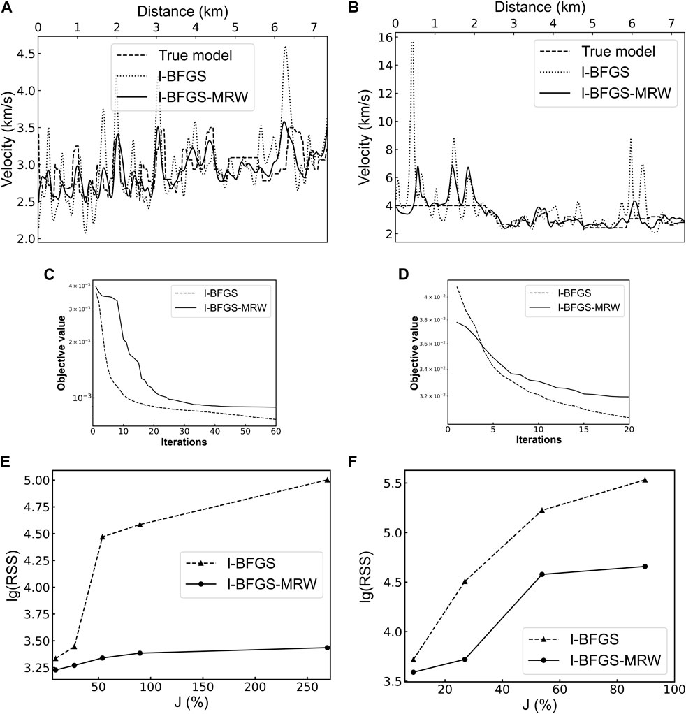
Figure 10. (A) The velocities extracted along a line (Distance = 0–7.335 km, Depth = 2.25 km) in Figures 7A, 9A, B; (B) the velocities extracted along a line (Distance = 0–7.335 km, Depth = 1.98 km) in Figures 7A, 9C, D; (C) the data convergence of 7–10 Hz inversion for Figures 9A, B; (D) the data convergence of 7–10 Hz inversion for Figures 9C, D; (E) lg(RSS) curve with J for 1–6 Hz inversion; (F) lg(RSS) curve with J for 7–10 Hz inversion.

Table 1

Table 1. The RSS of the inversion models specified by the tags and the true model.

The data convergence for Figures 9A, B is illustrated in Figures 10C, D shows the data convergence for Figures 9C, D. As shown in Figures 8E, 10C, D, the objective values of l-BFGS-MRW converge quickly, while the objective values of l-BFGS can barely converge even in a long iteration epoch. The RSS of the 1–6 Hz and 7–10 Hz inversion results are plotted as a function of J in Figures 10E, F, respectively. In comparison to the l-BFGS inversion, our FWI is not susceptible to data noise.

FWI is a time-consuming inversion technique, in which LU factorization (Equation 3) of the Helmholtz operator matrix accounts for most of the total time. L⁻¹ and U⁻¹ were stored after LU factorization for solving the wavefield using Equations 4, 5. In the FWI with l-BFGS-MRW, we could use L⁻¹ and U⁻¹ to solve the MRW without conducting an additional LU factorization. We did not need to calculate a series of reconstructed wavefields (Equation 12) and add them to obtain the MRW. According to Equation 14, we loaded a series of reconstruction sources at the same time to obtain the MRW, which costed the same time as calculating a single reconstructed wavefield. In FWI, a suitable search method can help quickly find the appropriate step length to save calculation time. The line search method for the step length employed in this work satisfied the strong Wolfe conditions as shown in Equations 19, 20 (Nocedal and Wright, 1999). During the inversion process, the step length was dynamically adjusted according to the number of the searches and the objective values. In theory, the total time consumption of our FWI is approximately 1.5 times that of l-BFGS FWI at the same iterations. When the noise is strong in the data, in addition to the time for solving the reconstructed wavefield, the l-BFGS-MRW inversion will cost more calculation time than the l-BFGS inversion in searching for the right step size to reduce the data residuals. The time spent on searching the step lengths accounts for most of the additional time. In some cases, such as that shown in Figures 8E, 10C, D, l-BFGS-MRW inversion requires less computational time than l-BFGS inversion because the objective value of l-BFGS-MRW converges much faster than that of l-BFGS, and we can stop the iteration of l-BFGS-MRW when the convergence occurs.

4 Discussion

The demand for oil and gas resources has prompted the development of deep and ultra-deep reservoirs. It is challenging for conventional FWI to obtain high-resolution deep or ultra-deep subsurface structures, particularly when the observational data is contaminated by non-Gaussian noise (Virieux and Operto, 2009; Brossier et al., 2009b; Asnaashari et al., 2013). Nevertheless, the l-BFGS-MRW inversion method has the potential to yield relatively accurate results with regard to deep stratigraphic structures. As illustrated in Figures 9A, B, the l-BFGS-MRW inversion is capable of achieving comparable precision to the l-BFGS inversion in the shallow region of the model. In the deep part of the model, the majority of deep wavefield components are unable to propagate to the surface and be received by the geophones. Consequently, this part of the deep components does not contribute to the FWI. Furthermore, the dot product of these components with the noise-based adjoint wavefield represents an artifact in the FWI gradient. The updates to the deep part of the model are primarily based on the reflected waves (Lian et al., 2018; Dong et al., 2018; Yao et al., 2020). The MRW is obtained by superimposing the reconstructed wavefield, thereby enhancing the reflected waves. The FWI gradient calculated with the enhanced reflected waves can effectively mitigate the impact of data noise-induced artifacts. Consequently, the l-BFGS-MRW inversion is capable of effectively resisting data noise and obtaining relatively accurate results in the deep part of the model (as illustrated in Figures 7D, F, H, Figures 9B, D). The use of MRW in FWI prevents data overfitting and increases the robustness of the inversion process, as shown in Figures 8A, B, 10A, B.

In general, the deep part of the initial velocity model can be effectively provided by the reflection full waveform inversion (Xu et al., 2012; Dong et al., 2018; Yao et al., 2020). An accurate deep structure can be obtained by combining reflection full waveform inversion with FWI (Cui et al., 2017). Our inversion method is capable of obtaining high-resolution deep velocity structure without reliance on the reflection full waveform inversion technique. Furthermore, it is resilient to noise interference. It should be noted that the data utilized in the experiment is synthetic data. Subsequent efforts will be made to apply our inversion method to actual detection data.

5 Conclusion

We develop a method to reconstruct a wavefield using the Helmholtz operator matrix and the first type of Rayleigh–Sommerfeld integral. In addition, we establish the multiple reconstructed wavefield (MRW) by stacking the reconstructed wavefields. The reflected waves of the MRW are enhanced relative to the other components. In the depth of the model, the enhanced reflected waves can dominate the calculation of the FWI gradient, suppressing artifacts created by data noise. The difference between the MRW and the original wavefield can effectively suppress the FWI fitting data noise. Therefore, calculating the gradient of the FWI using the MRW can mitigate the influence of data noise on the FWI. We employ the MRW to optimize the gradient of the FWI for improving the robustness of the FWI. Numerical experiments have proven that the MRW can help FWI avoid falling into the minimum caused by data noise and maintain a relatively high resolution. The l-BFGS inversion utilizing the MRW can obtain a stable model even though the input data is heavily affected by noise. Given that the L₁-norm penalty can hardly be combined with l-BFGS to handle noisy data in the FWI, the MRW provides an anti-noise method for the FWI with l-BFGS.

Data availability statement

The raw data supporting the conclusions of this article will be made available by the authors, without undue reservation.

Author contributions

YY: Writing–original draft. ZW: Writing–review and editing. XJ: Funding acquisition, Writing–review and editing. CZ: Writing–review and editing.

Funding

The author(s) declare that financial support was received for the research, authorship, and/or publication of this article. This study received support from the National Natural Science Foundation of China (42074125) and Sinopec Key Laboratory of Seismic Elastic Wave Technology Open Fund Project (33550000–22-ZC0613-0298).

Acknowledgments

We are very grateful to Dr. John T. Etgen, Alison Malcolm, Louise Alexander, Dr. Rene-Edouard Plessix and Dr. Michal Malinowski for their help, and their helpful comments have effectively improved this paper.

Conflict of interest

The authors declare that the research was conducted in the absence of any commercial or financial relationships that could be construed as a potential conflict of interest.

Publisher’s note

All claims expressed in this article are solely those of the authors and do not necessarily represent those of their affiliated organizations, or those of the publisher, the editors and the reviewers. Any product that may be evaluated in this article, or claim that may be made by its manufacturer, is not guaranteed or endorsed by the publisher.

References

Alkhalifah, T., and Choi, Y. (2012). Taming waveform inversion non-linearity through phase unwrap-ping of the model and objective functions. Geophys. J. Int. 191 (3), 1171–1178. doi:10.1111/j.1365-246X.2012.05699.x

CrossRef Full Text | Google Scholar

Alkhalifah, T., and Wu, Z. (2016). Multiscattering inversion for low-model wavenumbers. Geophysics 81, R417–R428. doi:10.1190/geo2015-0650.1

CrossRef Full Text | Google Scholar

Andrew, G., and Gao, J. (2007). Scalable training of L₁-regularized log-linear models. New York, NY, USA: Association for Computing Machinery, 33–40.

CrossRef Full Text | Google Scholar

Asnaashari, A., Brossier, R., Garambois, S., Audebert, F., Thore, P., and Virieux, J. (2013). Regularized seismic full waveform inversion with prior model information. Geophysics 78, R25–R36. doi:10.1190/geo2012-0104.1

CrossRef Full Text | Google Scholar

Berkhout, A. J. (1984). Seismic migration: imaging of acoustic energy by wave field extrapolation. Netherlands: Elsevier, 117–123.

Google Scholar

Berryhill, J. R. (1979). Wave-equation datuming. Geophysics 44, 1329–1344. doi:10.1190/1.1441010

CrossRef Full Text | Google Scholar

Born, M., and Wolf, E. (1999). Principles of optics: electromagnetic theory of propagation, interference and diffraction of light. 7th expanded ed. Cambridge University Press.

Google Scholar

Brossier, R., Operto, S., and Virieux, J. (2009a). Seismic imaging of complex onshore structures by 2D elastic frequency-domain full-waveform inversion. Geophysics 74, WCC105–WCC118. doi:10.1190/1.3215771

CrossRef Full Text | Google Scholar

Brossier, R., Operto, S., and Virieux, J. (2009b). Robust elastic frequency-domain full-waveform inver-sion using the L₁ norm. Geophys. Res. Lett. 36. doi:10.1029/2009gl039458

CrossRef Full Text | Google Scholar

Brossier, R., Operto, S., and Virieux, J. (2010). Which data residual norm for robust elastic frequency-domain full waveform inversion. Geophysics 75, R37–R46. doi:10.1190/1.3379323

CrossRef Full Text | Google Scholar

Bunks, C., Saleck, F., Zaleski, S., and Chavent, G. (1995). Multiscale seismic waveform inversion. Geophysics 60, 1457–1473. doi:10.1190/1.1443880

CrossRef Full Text | Google Scholar

Byrd, R. H., Nocedal, J., and Schnabel, R. B. (1994). Representations of quasi-Newton matrices and their use in limited memory methods. Math. Program. 63, 129–156. doi:10.1007/bf01582063

CrossRef Full Text | Google Scholar

Chen, B., and Jia, X. (2014). Staining algorithm for seismic modeling and migration. Geophysics 79, S121–S129. doi:10.1190/geo2013-0262.1

CrossRef Full Text | Google Scholar

Choi, Y., and Alkhalifah, T. (2012). “Frequency-domain waveform inversion using the unwrapped phase: expanded Abstracts,” in 81st Annual International Meeting (Houston, TX: Society of Exploration Geophysicists), 2576–2580.

CrossRef Full Text | Google Scholar

Claerbout, J. F. (1985). Imaging the earth’s interior. Oxford: Blackwell Scientific Publications.

Google Scholar

Constable, C. G. (1988). Parameter estimation in non-Gaussian noise. Geophys. J. 94 (1), 131–142. doi:10.1111/j.1365-246x.1988.tb03433.x

CrossRef Full Text | Google Scholar

Cui, C., Huang, J. P., Li, Z. C., Liao, W.-Z., and Guan, Z. (2017). Reflection full-waveform inversion using a modified phase misfit function. Appl. Geophys. 14, 407–418. doi:10.1007/s11770-017-0630-0

CrossRef Full Text | Google Scholar

Dai, M., Chen, J., and Cao, J. (2017). L₁-Regularized full-waveform inversion with prior model information based on orthant-wise limited memory quasi-Newton method. J. Appl. Geophys. 142, 49–57. doi:10.1016/j.jappgeo.2017.03.020

CrossRef Full Text | Google Scholar

da Silva, S. L. E. F., Costa, F. T., Karsou, A., de Souza, A., Capuzzo, F., Moreira, R. M., et al. (2024). Refraction FWI of a circular shot OBN acquisition in the Brazilian presalt region. IEEE Trans. Geoscience Remote Sens. 62, 1–18. doi:10.1109/tgrs.2024.3426956

CrossRef Full Text | Google Scholar

da Silva, S. L. E. F., and Kaniadakis, G. (2022). κ-statistics approach to optimal transport waveform inversion. Phys. Rev. E 106, 034113. doi:10.1103/physreve.106.034113

PubMed Abstract | CrossRef Full Text | Google Scholar

Dong, L., Fang, Z., Wang, H., Chi, H., and Liu, Y. (2018). Correlation-based reflection waveform inversion by one-way wave equations. Geophys. Prospect. 66, 1503–1520. doi:10.1111/1365-2478.12668

CrossRef Full Text | Google Scholar

Lailly, P. (1983). “The seismic inverse problem as a sequence of before stack migrations, Expanded Abstracts,” in Conference on inverse scattering, theory and application. Editors J. B. Bednar, E. Robinson, and A. Weglein (Philadelphia, PA: Society for Industrial and Applied Mathematics), 206–220.

Google Scholar

Li, Q., and Jia, X. (2017). Generalized staining algorithm for seismic modeling and migration. Geophysics 82, T17–T26. doi:10.1190/geo2015-0652.1

CrossRef Full Text | Google Scholar

Lian, S., Yuan, S., Wang, G., Liu, T., Liu, Y., and Wang, S. (2018). Enhancing low-wavenumber com-ponents of full-waveform inversion using an improved wavefield decomposition method in the time-space domain. J. Appl. Geophys. 157, 10–22. doi:10.1016/j.jappgeo.2018.06.013

CrossRef Full Text | Google Scholar

Métivier, L., Brossier, R., Operto, S., and Virieux, J. (2012). “Second-order adjoint state methods for full waveform inversion,” in Extended abstracts, 74st conference and exhibition, EAGE, hal-00826614.

Google Scholar

Mora, P. (1987). Nonlinear two-dimensional elastic inversion of multi-offset seismic data. Geophysics 52, 1211–1228. doi:10.1190/1.1442384

CrossRef Full Text | Google Scholar

Mora, P. (1988). Elastic wavefield inversion of reflection and transmission data. Geophysics 53, 750–759. doi:10.1190/1.1442510

CrossRef Full Text | Google Scholar

Nocedal, J., and Wright, S. J. (1999). Numerical optimization. New York: Springer-Verlag.

Google Scholar

Plessix, R.-E. (2006). A review of the adjoint-state method for computing the gradient of a functional with geophysical applications. Geophys. J. Int. 167, 495–503. doi:10.1111/j.1365-246x.2006.02978.x

CrossRef Full Text | Google Scholar

Poncet, R., Messud, J., Bader, M., Lambaré, G., Viguier, G., and Hidalgo, C. (2018). “FWI with optimal transport: a 3D implementation and an application on a field dataset, Expanded Abstracts,” in 80th EAGE conference and exhibition, 1–5.

Google Scholar

Pratt, R. G., Song, Z. M., Williamson, P. R., and Warner, M. (1996). Two-dimensional velocity models from wide-angle seismic data by wavefield inversion. Geophys. J. Int. 124, 323–340. doi:10.1111/j.1365-246x.1996.tb07023.x

CrossRef Full Text | Google Scholar

Pratt, R. G., and Worthington, M. H. (1990). Inverse theory applied to multisource cross-hole tomography, part 1: acoustic wave-equation method. Geophys. Prospect. 38, 287–310. doi:10.1111/j.1365-2478.1990.tb01846.x

CrossRef Full Text | Google Scholar

Shin, C., and Ha, W. (2008). A comparison between the behavior of objective functions for waveform inversion in the frequency and Laplace domains. Geophysics 73, VE119–VE133. doi:10.1190/1.2953978

CrossRef Full Text | Google Scholar

Sirgue, L., and Pratt, R. G. (2004). Efficient waveform inversion and imaging: a strategy for selecting temporal frequencies. Geophysics 69, 231–248. doi:10.1190/1.1649391

CrossRef Full Text | Google Scholar

Smith, J. A., Borisov, D., Cudney, H., Miller, R. D., Modrak, R., Moran, M., et al. (2019). Tunnel detection at Yuma Proving Ground, Arizona, USA—Part 2: 3D full-waveform inversion experiments. Geophysics 84, B107–B120. doi:10.1190/geo2018-0599.1

CrossRef Full Text | Google Scholar

Tarantola, A. (1984). Inversion of seismic reflection data in the acoustic approximation. Geophysics 49, 1259–1266. doi:10.1190/1.1441754

CrossRef Full Text | Google Scholar

Tejero, C. E. J., Dagnino, D., Sallar‘es, V., and Ranero, C. R. (2015). Comparative study of objective functions to overcome noise and bandwidth limitations in full waveform inversion. Geophys. J. Int. 203, 632–645. doi:10.1093/gji/ggv288

CrossRef Full Text | Google Scholar

Vigh, D., Moldoveanu, N., Jiao, K., Huang, W., and Kapoor, J. (2013). Ultralong-offset data acquisition can complement full-waveform inversion and lead to improved subsalt imaging. Lead. Edge 32, 1116–1122. doi:10.1190/tle32091116.1

CrossRef Full Text | Google Scholar

Vigh, D., and Starr, E. W. (2008). 3D prestack plane-wave, full-waveform inversion. Geophysics 73, VE135–VE144. doi:10.1190/1.2952623

CrossRef Full Text | Google Scholar

Virieux, J., and Operto, S. (2009). An overview of full waveform inversion in exploration geophysics. Geophysics 74, WCC1–WCC26. doi:10.1190/1.3238367

CrossRef Full Text | Google Scholar

Wang, L., Meng, D., and Wu, B. (2021). Seismic inversion via closed-loop fully convolutional residual network and transfer learning. Geophysics 86, R671–R683. doi:10.1190/geo2020-0297.1

CrossRef Full Text | Google Scholar

Wu, B.-Y., Wu, R.-S., Gao, J.-H., and Xu, Z.-B. (2017). Survey sinking migration using the time-space localized dreamlet one-way propagator. Chin. J. Geophys. 60 (9), 3505–3517. doi:10.6038/cjg20170919

CrossRef Full Text | Google Scholar

Wu, R.-S., Luo, J., and Wu, B. (2013). “Ultra-low-frequency information in seismic data and envelope inversion,” in Expanded abstracts, 83th annual international meeting (Houston, TX: Society of Exploration Geophysicists), 3078–3082.

Google Scholar

Wu, R.-S., Luo, J., and Wu, B. (2014). Seismic envelope inversion and modulation signal model. Geophysics 79, WA13–WA24. doi:10.1190/geo2013-0294.1

CrossRef Full Text | Google Scholar

Xie, C., Qin, Z. L., Wang, J. H., Song, P., Shen, H. G., Yu, S. Q., et al. (2024). Full waveform inversion based on hybrid gradient. Petroleum Sci. 21, 1660–1670. doi:10.1016/j.petsci.2024.01.013

CrossRef Full Text | Google Scholar

Xu, S., Wang, D., Chen, F., Lambaré, G., and Zhang, Y. (2012). “Inversion on reflected seismic wave,” 82nd Annual International Meeting (Houston, TX: Society of Exploration Geophysicists), 1–7.

Google Scholar

Yao, G., Wu, D., and Wang, S.-X. (2020). A review on reflection-waveform inversion. Petroleum Sci. 17, 334–351. doi:10.1007/s12182-020-00431-3

CrossRef Full Text | Google Scholar

Yu, Y., and Jia, X. (2021). “A frequency-domain staining algorithm for full waveform inversion with low SNR data,” in Extended abstracts, 82nd conference and exhibition, EAGE, 1–5.

Google Scholar