Spatial prediction of ground substrate thickness in shallow mountain area based on machine learning model

Introduction: The thickness of ground substrate in shallow mountainous areas is a crucial indicator for substrate investigations and a key factor in evaluating substrate quality and function. Reliable data acquisition methods are essential for effective investigation.

Methods: This study utilizes six machine learning algorithms—Gradient Boosting Machine (GB), Random Forest (RF), AdaBoost Regressor (AB), Neural Network (NN), Support Vector Machine (SVM), and k-Nearest Neighbors (kNN)—to predict ground substrate thickness. Grid search optimization was employed to fine-tune model parameters. The models’ performances were evaluated using four metrics: mean squared error (MSE), root mean squared error (RMSE), mean absolute error (MAE), and the coefficient of determination (R²). The optimal parameter combinations for each model were then used to calculate the spatial distribution of ground substrate thickness in the study area.

Results: The results indicate that after parameter optimization, all models showed significant reductions in the MSE, RMSE, and MAE, while R² values increased substantially. Under optimal parameters, the RF model achieved an MSE of 1,589, RMSE of 39.8, MAE of 26.5, and an R² of 0.63, with a Pearson correlation coefficient of 0.80, outperforming the other models. Therefore, parameter tuning is a necessary step in using machine learning models to predict ground substrate thickness, and the performance of all six models improved significantly after tuning. Overall, ensemble learning models provided better predictive performance than other machine learning models, with the RF model demonstrating the best accuracy and robustness.

Discussion: Moreover, further attention is required on the characteristics of sample data and environmental variables in machine learning-based predictions.

1 Introduction

The ground substrate layer serves as the fundamental material that nurtures and supports various natural resources at the Earth’s surface. Investigations focusing on this layer have been carried out in many parts of China (Hou et al., 2021; Jia et al., 2022). However, the content and methods of these surveys are still in the exploratory stage, and classifications and technical procedures have yet to be standardized (Dong et al., 2023; Li et al., 2023). In shallow mountain areas, the thickness of the ground substrate is an important indicator in ground substrate surveys and is a key factor in assessing the quality and function of the ground substrate (Yuan et al., 2023). It is widely applied in hydrology, ecology, and geological disaster prevention (Catani et al., 2010; Liu et al., 2019). The thickness of the ground substrate overlaps conceptually with soil thickness, weathered layer thickness, and the depth of the Earth’s critical zone, but there are differences. The depth of the ground substrate should consider the range that nurtures natural re-sources, with a focus in shallow mountain on the lower limit depth reached by super-gene geological processes dominated by weathering (Yin et al., 2020; Yao et al., 2022). Therefore, it is appropriate to define the thickness of the ground substrate as the depth from the surface to the interface of weakly weathered bedrock. Traditional survey methods primarily involve excavation and actual measurement, but these can cause ecological and environmental damage and are excessively costly. Using geophysical methods for exploration allows for the depiction of underground structures with relatively high precision, such as ground-penetrating radar, electrical resistivity tomography, seismic waves, and electromagnetic induction inversion (St. Clair et al., 2015; Tao et al., 2022). St. Clair et al. (2015) contend that terrestrial geophysical observations are typically limited to transects that extend hundreds of meters to a few kilometers in length and allow for investigation of local phenomena but do not have the broad view needed to characterize regional features that have length scales of several kilometers or more observations.

With the development of computer technology, modeling methods have been widely used in surveys of thickness for soil, sediments, and other substrates. These modeling methods can be divided into physically based models and stochastic statis-tical models. Dietrich et al. (1995) based on the law of mass balance between soil production from underlying bedrock and the divergence of diffusive soil transport, established a numerical model based on DEM (Digital Elevation Model) to predict soil depth. Fur-ther developed physical models of soil transport include soil diffusion models and fluvial sediment erosion transport models. Soil linear and nonlinear diffusion models relate soil diffusion to slope, curvature, and morphology (Culling, 1963; Roering, 2008; Pelletier and Rasmussen, 2009), while the flux of flu-vial sediment erosion transport can be proportionally related to watershed area and slope (Willgoose et al., 1991). However, there is still a lack of widely adopted soil thickness prediction models based on the theory of geomorphic evolution dynamics (Liu et al., 2024; Pelletier and Rasmussen, 2009). Building quantitative models of the ground substrate and landscape environmental factors for representative regions to predict the spatial distribution of ground substrate attributes is of great significance (Zhang et al., 2020).

Stochastic statistical models are based on a fundamental assumption that the relationship between soil properties of the samples and environmental variables can be extended to infer the soil properties of another location (Liu et al., 2019), which mainly includes regression algorithms, geostatistical methods, and machine learning models. Due to the nonlinear relationship between the thickness of the ground substrate and the relevant covariates (Roering, 2008), traditional regression algorithms and geostatistical methods seem to be inadequate for such complex calculations, leading to the widespread application of machine learning models (Liu et al., 2024). Machine Learning models, which do not require consideration of the complex mechanisms of ground substrate evolution, have the advantages of simple structure and fewer parameters (Wadoux et al., 2020), and have been widely applied in recent years to predict the thickness of soil and slope sediments (Shary et al., 2017; Jia et al., 2023). Machine learning, a subfield of artificial intelligence that emerged in the 1990s, is widely used in data mining and pattern recognition (Padarian et al., 2019a; Wadoux et al., 2020). At present, researchers widely adopt supervised learning methods for the prediction of ground substrate thickness, and commonly used algorithms include decision trees, support vector machines, k-nearest neighbor algorithms, neural networks, etc. For instance, Shen et al. (2022) successfully predicted the spatial distribution of soil texture in southern Ningxia using the random forest algorithm, and Shai et al., 2022 effectively predicted the thickness of aeolian sand in the Bashang area of Hebei using artificial neural network interpolation methods. Some researchers have also used other machine learning methods to construct models and achieve their research objectives (Qiu et al., 2020; Jin and Lv, 2022). In terms of application effectiveness, ensemble learning algorithms based on decision trees (such as random forests) are not sensitive to sample size and have good stability (Wadoux et al., 2020), neural networks have strong non-linear fitting capabilities, support vector machines are suitable for high-dimensional data (Huang et al., 2020), and k-nearest neighbor algorithms are simple and easy to implement. However, machine learning models have been less applied in the research on the prediction of ground substrate thickness, and there is a lack of necessary validation for the necessity of parameter optimization in related studies, which has not achieved the optimal performance of the models.

This study takes into account the technical characteristics of different machine learning models and selects six machine learning algorithms: Gradient Boosting (GB), Random Forest (RF), AdaBoost Regressor (AB), Neural Networks (NN), Support Vector Machine (SVM), and k-Nearest Neighbors (kNN) for the spatial prediction of ground substrate thickness in Ninghai County. Through grid search techniques, the parameters of each model were optimized to achieve the best model performance. Furthermore, the performance of the six models under optimal parameter combinations was compared and analyzed. The study also discusses the distribution patterns of ground substrate thickness in Ninghai county, providing a reference for exploring methods suitable for investigating ground substrate thickness.

2 Materials and methods

2.1 Study site

Ninghai county is located in the southern coastal area of Ningbo city in the eastern part of Zhejiang Province, China. It is geographically positioned was 29°06′∼ 29°32′N, 121°09′∼ 121°49′E. The elevation ranges from 0 to 926 m above sea level, covering a total area of 1,843 square kilometers. The county experiences a subtropical monsoon humid climate with an annual average temperature between 15.3°C and 17°C and annual rainfall ranging from 1,000 to 1,600 mm. The vegetation in Ninghai is predom-inantly composed of artificial coniferous forests, bamboo plantation, economic forests, and a small amount of secondary broadleaf forests. Remnants of the zonal subtropical evergreen broadleaf forests are preserved in the remote mountainous areas (Lan and Cheng, 2017). Lo-cated between the Tiantai and Siming mountain ranges, Ninghai features a coastal hilly terrain that is high in the west and low in the east, with the eastern part mainly con-sisting of low hills and alluvial plains. The region has been geologically active since the Late Mesozoic Cretaceous period, experiencing intense volcanic activity and under-going two major tectonic and magmatic phases during the Yanshanian and Himalayan periods. The geological makeup is predominantly mid-acidic Mesozoic volcanic rocks, followed by Neogene basic volcanic rocks (Yu et al., 2021). The surface substrate in the shallow mountain areas primarily consists of soils formed from the weathering and erosion of mid-acidic and basic volcanic rocks. The main ground substrate structure is soil and weathered bedrock, with thicknesses ranging from several centimeters to several me-ters. The substrate tends to be thinner in the upper slopes and thicker near the lower slopes and foothills.

2.2 Data sources and processing

2.2.1 Data sources

Ground substrate thickness data was obtained from field surveys by setting up a 30 m×30 m grid. To ensure the representativeness of the data, sampling grids are chosen to include continuous profiles and representative points, such as different landform types and geological backgrounds. The thickness data were collected using profile surveys and backpack drilling. The average thickness value for each grid area was then calculated, yielding a total of 290 survey points, including 267 outcrop survey points and 23 backpack drill sites. The locations of the survey points are shown in Figure 1. The topographic data were sourced from the National Geographic Information Center’s DEM data (https://ngcc.cn/ngcc/), with a resolution of 30 m×30 m in a raster format, encompassing a total of 1,905,951 grids. Geological environment variables were derived from a 1:250,000 geological map that was updated and compiled, primarily considering the rock types of geological units. These vector graphics were converted into raster files using ArcGIS 10.8 software to obtain geological data.

Figure 1

Figure 1. Topography of Ninghai County and sampling locations.

2.2.2 Data processing

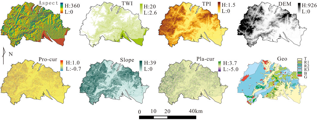
Using DEM data, environmental variables such as slope, aspect, plan curvature, and profile curvature can be calculated. Terrain Wetness Index (TWI) and Topographic Position Index (TPI) are important indicators in studies related to soil evolution and slope sedimentation (Ziadat, 2010; Shary et al., 2017; Sharififar et al., 2019). In this study, TWI and TPI were calculated using DEM data and utilized as significant environmental variables. By transforming the data formats, different layers in ArcGIS were uniformly created, and the spatial distribution characteristics of the main environmental variables are shown in Figure 2. Discrete data types in the environmental variables include geological rock classification (Geo) and slope, with seven categories for geological classification and division of aspect into eight directions based on 45° intervals, and these data are all represented in text format. Continuous variables mainly include DEM, slope, plane curvature (Pla-cur), profile curvature (Pro-cur), TWI, and TPI, as described in Table 1. In the environmental variable data, there is a phenomenon of missing values for TWI, mainly occurring in ridge and steep slope areas, possibly due to anomalies in calculating slope direction and gradient from the DEM data. Since TWI is a continuous numerical variable, its impact on calculating the importance of TWI in ridge and steep slope areas is also minimal. For the missing values, the main approach is to fill them with “0”.

Figure 2

Figure 2. Grid and vector diagrams of major environmental variables in Ninghai county.

Table 1

Table 1. Characteristics of continuous environment variables.

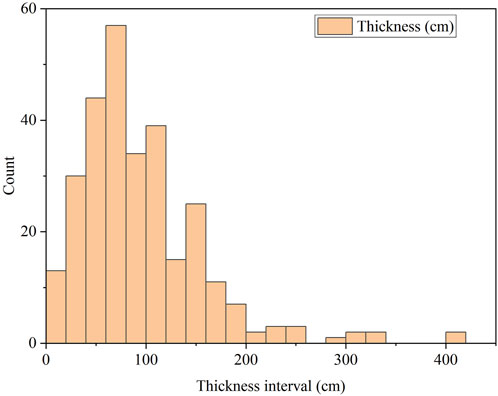
The sample data consists of 290 points of target variables and environmental variables. The environmental variable TWI also has missing values, which have been treated by filling them with “0”. The target variable (ground substrate thickness) has a range of 5–400 cm, with a mean value of 92.79 cm. Thickness is primarily distributed between 0 and 150 cm, ac-counting for 87.3% of the total data. The distribution of data across different thickness intervals is shown in Figure 3. The sample data is divided into a training set and a test set, using random sampling to select 80% as the training set and 20% as the test set. To ensure the reliability of the results, cross-validation is used for training and testing, with 10-fold cross-validation, thereby ensuring a sufficient amount of data to obtain more result data.

Figure 3

Figure 3. Statistical map of ground substrate thickness data.

2.3 Research methods

2.3.1 Machine learning models

2.3.1.1 Ensemble learning algorithms

Ensemble learning aims to improve overall prediction performance by combining the predictions of multiple base models. Common ensemble learning methods include Gradient Boosting Machine, Random Forest, and AdaBoost Regressor algorithms.

Gradient Boosting Machine (GB) is an ensemble learning method based on decision trees. It iteratively trains decision tree models to gradually improve the overall model performance (Friedman, 2002). It utilizes the loss function to compute the negative gradient of a randomly sampled subset for training a decision tree, known as the “pseudo-residual”. The pseudo-residual v_(π(i) at the tth iteration can be represented as:

${\mathit{v}}_{\mathit{\pi }\left(\mathit{i}\right)}={-\left[\frac{\partial \mathit{\Phi }\left({\mathit{y}}_{\mathit{\pi }\left(\mathit{i}\right)},\mathit{F}\left({\mathit{x}}_{\mathit{\pi }\left(\mathit{i}\right)}\right)\right)}{\partial \mathit{F}\left({\mathit{x}}_{\mathit{\pi }\left(\mathit{i}\right)}\right)}\right]}_{\mathit{F}\left(\mathit{x}\right)={\mathit{F}}_{\mathit{t}-\mathbf{1}}\left(\mathit{x}\right)}(1)$

In Equation 1, the loss function ∂Φ(y,F(x)) is differentiable; F(x) represents the current base learner; π(i) denotes a random sequence.

Random Forest (RF) is an ensemble learning method used for tasks such as classification and regression (Breiman, 2001). When developing an individual tree, a random subset of attributes is drawn, from which the best attribute for splitting is selected. The final model is based on a majority vote of the trees independently grown in the forest, and the final prediction result is obtained by averaging the results of all the trees, which can be expressed as:

$\mathit{F}\left(\mathit{x}\right)=\frac{\mathbf{1}}{\mathit{n}}{\displaystyle \sum _{\mathit{t}=\mathbf{1}}^{\mathit{n}}}{\mathit{h}}_{\mathit{t}}\left(\mathit{x}\right)(2)$

In Equation 2, F(x) represents the final prediction result of the Random Forest (RF), and h_t(x) denotes the regression prediction result of the tth decision tree.

AdaBoost Regressor (AB) algorithm is a method of iteratively training multiple weak regression models (Solomatine and Shrestha, 2004). It weights each model, and in each iteration, sample weights are adjusted to make the current model pay more attention to samples incorrectly predicted in the previous iteration. The final prediction result is the weighted average of all weak regression models.

2.3.1.2 Neural network algorithm

Neural Network (NN) utilizes the multilayer perceptron algorithm from sklearn, which can learn both nonlinear and linear models. Its structure consists of an input layer, one or more hidden layers, and an output layer (Wolpert, 1992). A single-layer perceptron has only input and output layers, so it can only learn linear functions, while a multi-layer perceptron has one or more hidden layers, allowing it to learn nonlinear func-tions as well.

2.3.1.3 Support vector machine (SVM) algorithm

Support Vector Machine (SVM) separates the attribute space using a hyperplane to maximize the margin between instances of different classes or different class values (Smola and Schölkopf, 2004). We utilize Support Vector Regression to minimize the total deviation of all sample points from the hyperplane.

$\left\{\begin{array}{l}\mathit{min}\frac{\mathbf{1}}{\mathbf{2}}{‖\mathit{w}‖}^{\mathbf{2}}\\ \mathit{s}.\mathit{t}.\left|{\mathit{y}}_{\mathit{i}}-\left(\mathit{w}{\mathit{x}}_{\mathit{i}}+\mathit{b}\right)\right|\le \mathit{\epsilon },\forall \mathit{i}\end{array}\right.(3)$

In Equation 3, w represents the normal vector of the hyperplane, b is the bias term, y_i is the target value of the ith sample, and x_i is the feature value of the ith sample.

2.3.1.4 K-Nearest Neighbors (kNN) algorithm

k-Nearest Neighbors (kNN) searches for the k nearest training samples in the feature space and uses their average as the prediction (Peterson, 2009). The kNN algorithm is based on distance metrics, determining the most similar k samples by computing distances between samples. In classification problems, the class of the sample is determined by a voting mechanism, while in regression problems, the output value of the sample is determined by averaging.

The primary parameters influencing model performance encompass the number of iterations (n_estimators) and learning rate (learning_rate) for GB, as well as the maximum depth of trees (max_depth); for RF, the count of decision trees (n_estimators) and the maximum tree depth (max_depth); for AB, the learning rate (learning_rate); for NN, the sizes and quantity of hidden layers (hidden_layer_sizes), along with the activation function (activation); for SVM, the choice of kernel function (kernel) and the regularization parameter (C); and for kNN, the number of neighbors (n_neighbors) and the exponent for distance calculation (p). These key parameters often directly affect the model’s complexity and generalization ability, potentially enhancing model performance but also possibly increasing model complexity and computational costs. The aforementioned algorithms are primarily implemented using the sklearn library on the Python platform.

2.3.2 Key parameter spaces

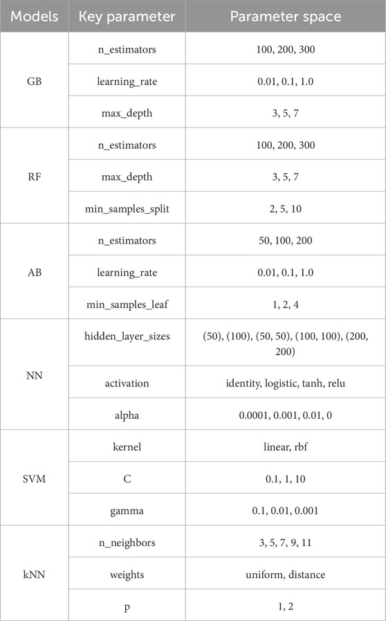
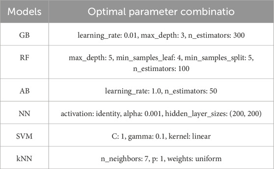
To optimize for the best model performance, methods such as grid search, random search, and Bayesian optimization are commonly used to fine-tune parameters. Random search has a relatively low cost but involves random selection, while Bayesian search is costly. This paper employs the grid search method to find the optimal parameter combination (Ottoy et al., 2017; Padarian et al., 2019a). Considering the impact of parameters on the model comprehensively,we set the parameter space for each machine learning model and use the grid search method to traverse the model performance under different parameters of each model. Table 2 lists the key parameters of different models, with values mainly considering common parameter ranges and computational efficiency (Padarian et al., 2019a). There are 27, 27, 27, 60, 18, and 20 parameter combinations for the six models respectively.

Table 2

Table 2. Lists of key parameters of each model.

2.3.3 Evaluation metrics

The prediction accuracy is primarily evaluated using four metrics: Mean Squared Error (MSE), Root Mean Squared Error (RMSE), Mean Absolute Error (MAE), and Coefficient of Determination (R²) (Minasny et al., 2018; Hamzehpour et al., 2019; Zeraatpisheh et al., 2019). RMSE is the square root of MSE, measuring the average error between the predicted values and the true values. MAE is the average of the absolute differences between the predicted values and the true values. R² is a metric used to measure the goodness of fit of the model to the data, indicating the proportion of variance explained by the model. The closer R² is to 1, the better the model fits the data. The formulas for evaluation metrics are as follows:

$\mathit{M}\mathit{S}\mathit{E}=\frac{\mathbf{1}}{\mathit{m}}{\displaystyle \sum _{\mathbf{i}=\mathbf{1}}^{\mathit{m}}}{\left({\mathit{y}}_{\mathit{i}}-\widehat{{\mathit{y}}_{\mathit{i}}}\right)}^{\mathbf{2}}(4)$

$\mathit{R}\mathit{M}\mathit{S}\mathit{E}=\sqrt{\mathit{M}\mathit{S}\mathit{E}}=\sqrt{\frac{\mathbf{1}}{\mathit{m}}{\displaystyle \sum _{\mathit{i}=\mathbf{1}}^{\mathit{m}}}{\left({\mathit{y}}_{\mathit{i}}-\widehat{{\mathit{y}}_{\mathit{i}}}\right)}^{\mathbf{2}}}(5)$

$\mathit{M}\mathit{A}\mathit{E}=\frac{\mathbf{1}}{\mathit{m}}\left|{\mathit{y}}_{\mathit{i}}-\widehat{{\mathit{y}}_{\mathit{i}}}\right|(6)$

${\mathit{R}}^{\mathbf{2}}=\mathbf{1}-\frac{{\sum }_{\mathit{i}}{\left(\widehat{{\mathit{y}}_{\mathit{i}}}-{\mathit{y}}_{\mathit{i}}\right)}^{\mathbf{2}}}{{\sum }_{\mathit{i}}{\left(\overline{\mathit{y}}-{\mathit{y}}_{\mathit{i}}\right)}^{\mathbf{2}}}(7)$

In the formulas (Equations 4–7), y_i represents the true value, $\widehat{{\mathit{y}}_{\mathit{i}}}$ represents the predicted value, and $\overline{\mathrm{y}}$ represents the sample mean.

3 Results

3.1 Parameter optimization

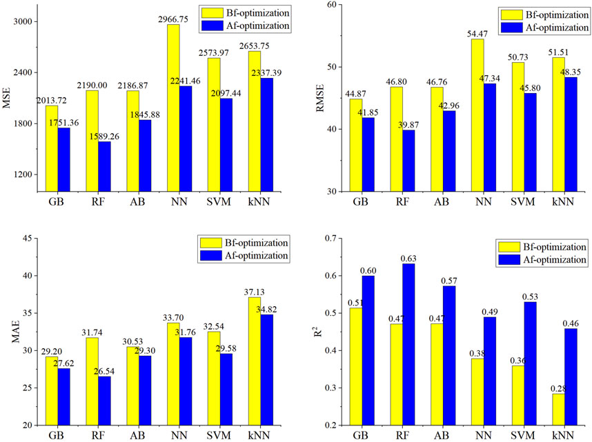
From the perspective of model evaluation metrics, before parameter optimization, using default parameters, the performance of ensemble learning models was moderate, while NN, SVM, and kNN models showed relatively poor performance. After param-eter optimization, the performance of all models improved significantly. MSE, RMSE, and MAE decreased noticeably, with reductions ranging from 262 to 725, 3.0 to 7.1, and 1.2 to 5.2, respectively. R² increased significantly, with increments ranging from 0.09 to 0.17. The models with the most significant decreases in MSE were mainly RF, NN, and SVM, with reductions of 600, 725, and 477, respectively. RF and NN showed the most substantial reductions in RMSE, decreasing by 6.9 and 7.1, respectively. RF exhibited the most substantial decrease in MAE, with a decrease of 5.2. The models with the most significant increases in R² were RF, SVM, and kNN, with improvements of 0.16, 0.17, and 0.17, respectively. Comparatively, RF showed the most significant improvement in performance, characterized by a significant decrease in various types of errors and an enhancement in linear fitting (Figure 4).

Figure 4

Figure 4. Changes of evaluation indexes after parameter optimization of each model.

Using the grid search method, the optimal parameter combinations for each model were selected, and the performance of each model varied significantly with different parameter selections (Table 3). With the optimal parameter combinations, the RF model exhibited the best performance, with the smallest errors and the highest co-efficient of determination. Specifically, MSE, RMSE, MAE, and R² were 1,589, 39.8, 26.5, and 0.63, respectively. The optimal parameters for the RF model were as follows: the number of decision trees was set to 100, the maximum depth of the decision trees was 5, the minimum number of samples required to split a node was 5, and the minimum number of samples required to be at a leaf node was 4.

Table 3

Table 3. Optimal parameter combination table of different models.

3.2 Model validation

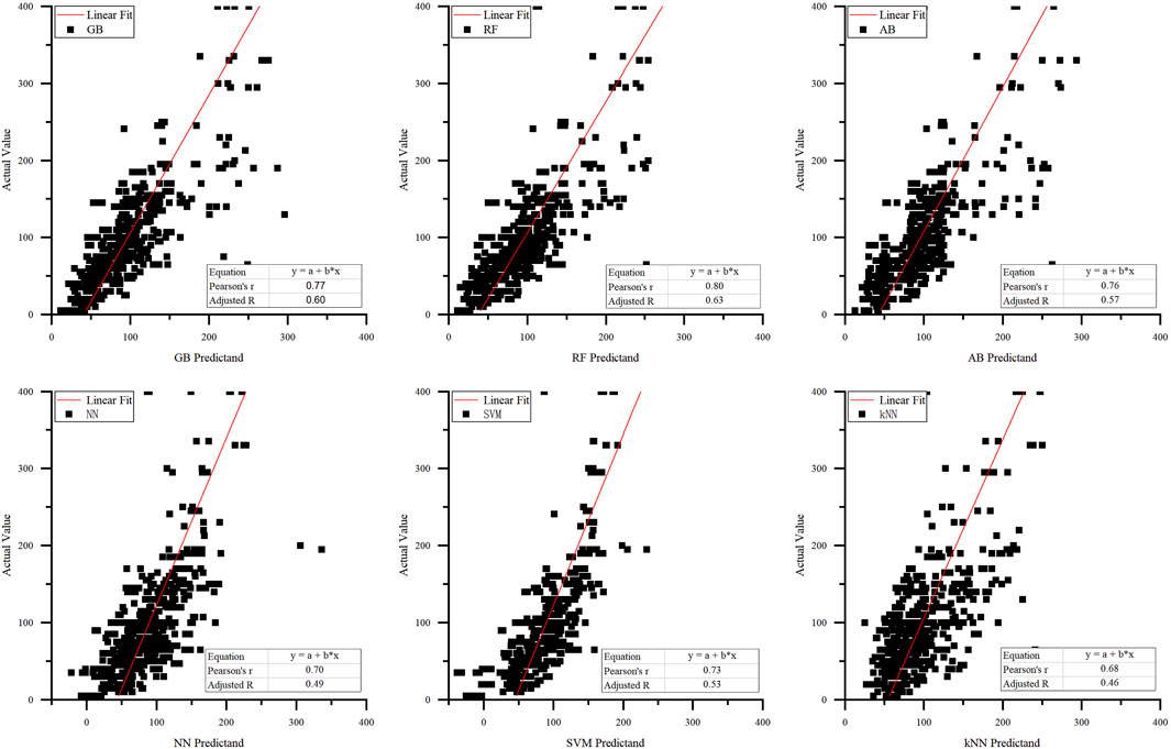
From the scatter plot in Figure 5, it can be observed that ensemble learning models (GB, RF, AB) exhibit relatively good fitting. Among them, RF demonstrates the best overall predictive fitting, with the highest pearson correlation coefficient of 0.80 and R² of 0.63. Both GB and AB show high dispersion in mid-range predictions. Conversely, NN and SVM predictions yield negative values, indicating an overall underestimation of thickness, while kNN predictions display higher dispersion and larger errors, with the lowest Pearson correlation coefficient of 0.68.

Figure 5

Figure 5. Scatter plot of test set prediction results.

3.3 Result mapping

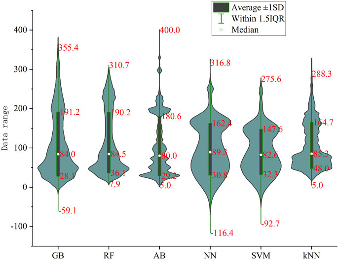
The predicted values of each model range from −116.4–400 cm. Among them, four models—GB, SVM, NN, and kNN—yield negative values. kNN and SVM gener-ally produce smaller predictions, while the AB model exhibits multiple peaks (Figure 6). The predictions of the RF and GB models are similar, closely resembling the distribu-tion of sample data. Both models peak around 50 and 200 cm, with an overall dis-tribution between 30 and 90 cm, and a median of approximately 84 cm. The pre-dictions of the AB model fluctuate significantly, showing multiple peaks. NN and SVM models produce notably negative values, resulting in overall underestimation of thickness, with distribution relatively even between 0 and 200 cm. The kNN pre-dictions exhibit two peaks overall, but the overall predicted values are lower.

Figure 6

Figure 6. Statistical map of ground substrate thickness prediction.

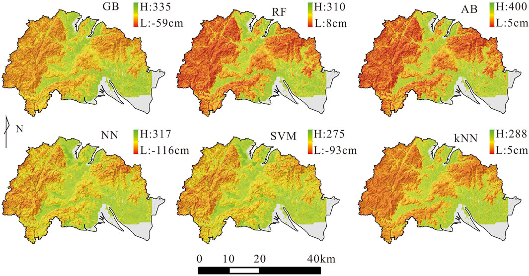
Based on the model predictions, grid values were assigned to generate a spatial map of ground substrate thickness (Figure 7). Overall, the spatial distribution of ground substrate thickness reveals that the 0–30 cm range is primarily located in steep mountain ridges and slopes. The 30–60 cm range predominates in the transitional areas from ridge to gentle slope. Areas with thickness ranging from 60 to 150 cm are mainly found on gentle hilltops and downhill slopes. Thicknesses ranging from 150 to 400 cm are mainly situated at the foot of slopes or on gently rolling hills. The pre-dicted thickness distribution aligns with field survey observations. Generally, thickness in mountainous regions ranges from 0 to 150 cm, while thickness is higher in low-gradient slope areas.

Figure 7

Figure 7. Predicted distribution of ground substrate thickness in Ninghai county.

4 Discussion

4.1 Parameter tuning method selection

The performance of a machine learning model is affected by its parameter values, and tuning the parameters can significantly improve model performance (Padarian et al., 2019b). Re-searchers generally optimize parameters for one or two models (Wu et al., 2016; Sergeev et al., 2019; Wadoux et al., 2019), Wadoux et al. (2020) found that nearly half of the literature in their sample statistics did not perform parameter tuning, and when comparing multiple models, default parameters are often used (Vermeulen and Van Niekerk, 2017; Minasny et al., 2018; Keskin et al., 2019). Through our study, it is evident that parameter tuning is necessary. We select the grid search method to traverse the parameter space, which still has certain limitations. When computational costs are permissible, Bayesian methods, genetic algorithms, particle swarm optimization, and other algorithms can be used for parameter optimization (Wu et al., 2016; Wadoux et al., 2019).

4.2 Comparative analysis of models

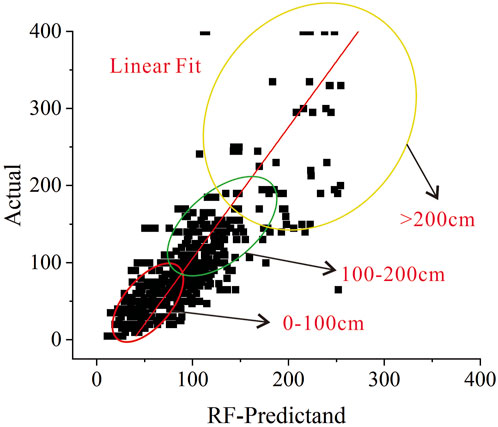
Wang Sheng. (2015) assessed the estimation of soil layer thickness using different methods, with R² values ranging from 0.39 to 0.66; whereas Kempen et al. (2011), when predicting organic carbon at different depths, had R² values from 0.09 to 0.75. Liu et al. (2013), within a small area, made high-precision spatial predictions of soil thickness based on geomorphology, with an R value of 0.74. Combining other relevant studies, we believe that R² values between 0.6 and 0.8 are considered to be relatively reliable (Ottoy et al., 2017; Minasny et al., 2018). By comparing the model training results, the RF model has good accuracy. From the perspective of various indicators, MSE, RMSE, and MAE are relatively small, re-flecting that the prediction results of the RF model have small errors, while R² is rela-tively large, indicating that the RF model has good stability and is generally consistent with the verification data. As shown in Figure 5, the prediction results of the RF model did not show negative values, and no excessive parameter adjustment is required. Secondly, from the model verification effect (Figure 8), the RF model showed good re-liability in the case of 0–100 and 100–200 cm thickness and more sample data; even if the thickness is greater than 200 cm and the sample data is less, it can maintain good ac-curacy and relatively low discreteness, indicating that the RF model has good robust-ness and wider applicability.

Figure 8

Figure 8. RF model test verification scatter plot.

4.3 The impact of other factors on the prediction results

In addition to the model, the quality of sample data and the selection of envi-ronmental variables are also important factors affecting the prediction of surface ma-trix thickness. Generally speaking, the larger the data volume and the higher the data quality, the more accurate the prediction results. During the field survey, due to the relatively thick coverage of the low and gentle slope areas, fewer field outcrops, and reduced sample size, the accuracy of each model decreased significantly. When the ground substrate thickness is small, all models perform well, but when the thickness is greater than 150 cm, the discreteness of the prediction increases significantly.

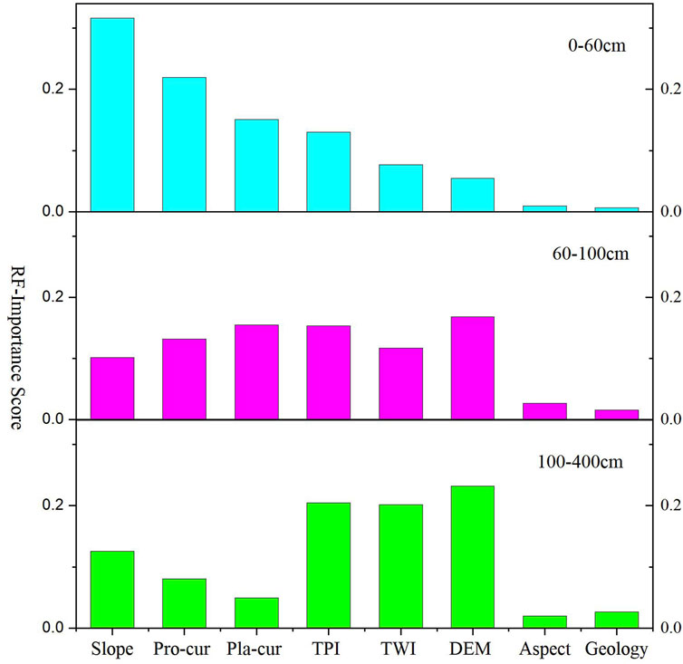
Because most ML models are complex in structure,. How to increase the interpretability of machine learning model predic-tions has always been an unresolved problem. Based on the data distribution charac-teristics, this paper divides the sample data into three groups according to thickness, namely, [0, 60] cm, [60, 100] cm, and [100, 300] cm, and then analyzes the importance of environmental variables at different thicknesses. The calculation results show (Figure 9) that there are obvious differences in the importance of each group of environmental variables, indicating that different variables have different effects on the evolution of the ground substrate. Therefore, future research should focus on the geological and ge-omorphological characteristics of the ground substrate and their mutual influence on the spatial distribution of the ground substrate thickness.

Figure 9

Figure 9. Importance scores of environmental variables at different thicknesses based on RF model.

5 Conclusion

In this study, surface material thickness data from 290 points were collected and used to construct models through different machine learning algorithms. By employing the grid search method, various parameter combinations were explored to find the optimal set. The performance of six models was compared and analyzed, and a spatial distribution map of surface material thickness in Ninghai County was generated. The discussion highlighted the necessity of parameter tuning and the strengths and weak-nesses of the models. It was also noted that the quality of sample data and the selection of covariates significantly affect the prediction results, warranting further attention in future research. The following conclusions were drawn from the study.

(1) Parameter tuning is essential for predicting surface material thickness using machine learning models. The performance of all six models improved significantly after parameter tuning. Using the grid search method for parameter tuning, the pre-diction errors of each model generally decreased, and the R² value significantly in-creased. Among the models, RF, NN, and SVM showed the most reduction in error, while RF, SVM, and kNN exhibited the most improvement in linear fit. This optimiza-tion provides the best parameter combinations, serving as a reference for subsequent practical predictions.

(2) Overall, ensemble learning models outperform other machine learning models in prediction accuracy. Among the ensemble models, RF demonstrated the highest accuracy and robustness. The ensemble models GB, AB, and RF all had relatively low prediction errors and high fitting degrees, with RF showing the best predictive per-formance: MSE, RMSE, MAE, and R² were 1,589, 39.8, 26.5, and 0.63, respectively, and the Pearson correlation coefficient was the highest at 0.80.

(3) Machine learning models can effectively predict surface material thickness in shallow mountainous areas, but further attention to sample data and environmental variables is necessary. The prediction results indicate that areas such as steep ridges generally have thinner surface materials, typically only a few dozen centimeters. In contrast, transitional zones such as gentle slopes tend to have thicker surface materials, reaching up to several hundred centimeters at the foot of slopes or in hilly areas, aligning with field survey observations. The predicted results for the entire Ninghai County also closely matched the distribution of sample data. Due to the study’s limi-tations, further research and analysis on sample data and environmental variables are needed through more investigative practices.

Data availability statement

The datasets presented in this article are not readily available because the data that support the findings of this study are not publicly available due to confidentiality agreements with participants and privacy concerns. However, the data can be made available by the corresponding authors upon reasonable request. Requests to access the datasets should be directed to zhuxiaosong@mail.cgs.gov.cn.

Author contributions

XZ: Conceptualization, Formal Analysis, Methodology, Project administration, Software, Validation, Visualization, Writing–original draft, Writing–review and editing. XP: Conceptualization, Writing–review and editing. SY: Conceptualization, Methodology, Software, Writing–review and editing. WW: Conceptualization, Methodology, Writing–review and editing. YD: Formal Analysis, Writing–review and editing. MF: Project administration, Writing–review and editing. WL: Project administration, Writing–review and editing. LJ: Methodology, Project administration, Writing–review and editing.

Funding

The author(s) declare that financial support was received for the research, authorship, and/or publication of this article. This research was funded by Science and Technology Innovation Foundation of Command Center of Integrated Natural Resources Survey Center, grant number KC20220010; Science and Tech-nology Innovation Foundation of Command Center of Integrated Natural Resources Survey Center, grant number KC20230018; China Geological Survey project, grant number ZD20220118; China Geological Survey project, grant numbers DD20242562 and DD20242768.

Acknowledgments

We thank the China Geological Survey for providing technical and financial support.

Conflict of interest

The authors declare that the research was conducted in the absence of any commercial or financial relationships that could be construed as a potential conflict of interest.

Publisher’s note

All claims expressed in this article are solely those of the authors and do not necessarily represent those of their affiliated organizations, or those of the publisher, the editors and the reviewers. Any product that may be evaluated in this article, or claim that may be made by its manufacturer, is not guaranteed or endorsed by the publisher.

Supplementary material

The Supplementary Material for this article can be found online at: https://www.frontiersin.org/articles/10.3389/feart.2024.1455124/full#supplementary-material

References

Breiman, L. (2001). Random forests. Mach. Learn. 45, 5–32. doi:10.1023/A:1010933404324

CrossRef Full Text | Google Scholar

Catani, F., Segoni, S., and Falorni, G. (2010). An empirical geomorphology-based approach to the spatial prediction of soil thickness at catchment scale. Water Resour. Res. 46 (5), W05508. doi:10.1029/2008WR007450

CrossRef Full Text | Google Scholar

Culling, W. (1963). Soil creep and the development of hillside slopes. J. Geol. 71 (2), 127–161. doi:10.1086/626891

CrossRef Full Text | Google Scholar

Dietrich, W. E., Reiss, R., Hsu, M. L., and Montgomery, D. R. (1995). A process-based model for colluvial soil depth and shallow landsliding using digital elevation data. Hydrol. Process. 9 (3-4), 383–400. doi:10.1002/HYP.3360090311

CrossRef Full Text | Google Scholar

Dong, T., Liu, X., Chang, M., Liyuan, X., and Ran, W. (2023). Analysis on the essential connotation and research direction of surface substrate. Northwest. Geol. 56 (4), 213–217. doi:10.12401/j.nwg.2023040

CrossRef Full Text | Google Scholar

Friedman, J. H. (2002). Stochastic gradient boosting. Comput. statistics and data analysis 38 (4), 367–378. doi:10.1016/S0167-9473(01)00065-2

CrossRef Full Text | Google Scholar

Hamzehpour, N., Shafizadeh-Moghadam, H., and Valavi, R. (2019). Exploring the driving forces and digital mapping of soil organic carbon using remote sensing and soil texture. Catena 182, 104141. doi:10.1016/j.catena.2019.104141

CrossRef Full Text | Google Scholar

Hou, H. X., Zhang, S. J., Lu, M., Zhang, Z. Y., Sun, X., and Qin, T. (2021). Technology and method of the ground substrate layer survey of natural resources: taking Baoding area as an example. Northwest. Geol. 54 (3), 277–288. doi:10.19751/j.cnki.61-1149/p.2021.03.026

CrossRef Full Text | Google Scholar

Huang, J. C., Ko, K. M., Shu, M. H., and Hsu, B. M. (2020). Application and comparison of several machine learning algorithms and their integration models in regression problems. Neural Comput. Appl. 32 (10), 5461–5469. doi:10.1007/s00521-019-04644-5

CrossRef Full Text | Google Scholar

Jia, L., Liu, H., OuYang, Y., Zhang, W., Dou, L., Liu, Z. N., et al. (2022). Division scheme of surface substrate mapping units of mountainous-hilly area in south China based on geological formations research: example from Xinhui-Taishan area in Pearl River Delta. Northwest. Geol. 55 (4), 140–157. doi:10.19751/j.cnki.61-1149/p.2022.04.013

CrossRef Full Text | Google Scholar

Jia, J., Mao, Y. M., Meng, X. J., Gao, B., Gao, M. X., and Wu, W. X. (2023). Comparison of landslide susceptibility evaluation by deep random forest and random forest model: a case study of Lueyang County, Hanzhong City. Northwest. Geol. 56 (3), 239–249. doi:10.12401/j.nwg.2023084

CrossRef Full Text | Google Scholar

Jin, Z., and Lv, J. S. (2022). Comparison of the accuracy of spatial prediction for heavy metals in regional soils based on machine learning models. Geogr. Res. 41 (6), 1731–1747. doi:10.11821/dlyj020210528

CrossRef Full Text | Google Scholar

Kempen, B., Brus, D. J., and Stoorvogel, J. J. (2011). Three-dimensional mapping of soil organic matter content using soil type–specific depth functions. Geoderma 162 (1-2), 107–123. doi:10.1016/j.geoderma.2011.01.010

CrossRef Full Text | Google Scholar

Keskin, H., Grunwald, S., and Harris, W. G. (2019). Digital mapping of soil carbon fractions with machine learning. Geoderma 339, 40–58. doi:10.1016/j.geoderma.2018.12.037

CrossRef Full Text | Google Scholar

Lan, X. C., and Cheng, L. (2017). Study on the regionalization of soil and water conservation in Ningbo City. SSWC 15 (1), 141–147. doi:10.16843/j.sswc.2017.01.018

CrossRef Full Text | Google Scholar

Li, X., Zhou, X., Xiang, Z., Ren, J., Bing, T., Dai, Z., et al. (2023). Simply discussion on the work of ground substrate survey: taking Hainan Island as an example. Geol. Bull. China 42 (1), 68–75. doi:10.12097/j.issn.1671-2552.2023.01.006

CrossRef Full Text | Google Scholar

Liu, J., Chen, X., Lin, H., Liu, H., and Song, H. (2013). A simple geomorphic-based analytical model for predicting the spatial distribution of soil thickness in headwater hillslopes and catchments. Water Resour. Res. 49 (11), 7733–7746. doi:10.1002/2013wr013834

CrossRef Full Text | Google Scholar

Liu, J., Han, X., Liu, J., Liang, Z., and He, R. (2019). Understanding of critical zone structures and hydrological connectivity: a review. Adv. Water Sci. 30 (1), 112–122. doi:10.14042/j.cnki.32.1309.2019.01.012

CrossRef Full Text | Google Scholar

Liu, J., Zhao, W., and Liu, Y. (2024). Modelling soil thickness evolution: advancements and challenges. Acta Pedol. Sin. 61 (2), 319–330. doi:10.11766/trxb202207070374

CrossRef Full Text | Google Scholar

Minasny, B., Setiawan, B. I., Saptomo, S. K., and McBratney, A. B. (2018). Open digital mapping as a cost-effective method for mapping peat thickness and assessing the carbon stock of tropical peatlands. Geoderma 313, 25–40. doi:10.1016/j.geoderma.2017.10.018

CrossRef Full Text | Google Scholar

Ottoy, S., De Vos, B., Sindayihebura, A., Hermy, M., and Van Orshoven, J. (2017). Assessing soil organic carbon stocks under current and potential forest cover using digital soil mapping and spatial generalisation. Ecol. Indic. 77, 139–150. doi:10.1016/j.ecolind.2017.02.010

CrossRef Full Text | Google Scholar

Padarian, J., Minasny, B., and McBratney, A. B. (2019a). Machine learning and soil sciences: a review aided by machine learning tools. Soil 6 (1), 35–52. doi:10.5194/soil-6-35-2020

CrossRef Full Text | Google Scholar

Padarian, J., Minasny, B., and McBratney, A. B. (2019b). Using deep learning for digital soil mapping. Soil 5 (1), 79–89. doi:10.5194/soil-5-79-2019

CrossRef Full Text | Google Scholar

Pelletier, J. D., and Rasmussen, C. (2009). Geomorphically based predictive mapping of soil thickness in upland watersheds. Water Resour. Res. 45 (9), W09417. doi:10.1029/2008WR007319

CrossRef Full Text | Google Scholar

Peterson, L. E. (2009). K-nearest neighbor. Scholarpedia 4 (2), 1883. doi:10.4249/scholarpedia.1883

CrossRef Full Text | Google Scholar

Qiu, W., Wu, B., Pan, X., and Tang, Y. (2020). Application of several cluster-optimization-based machine learning methods in evaluation of landslide susceptibility in Lingtai County. Northwest. Geol. 53 (1), 222–233. doi:10.19751/j.cnki.61-1149/p.2020.01.021

CrossRef Full Text | Google Scholar

Roering, J. J. (2008). How well can hillslope evolution models “explain” topography? Simulating soil transport and production with high-resolution topographic data. Geol. Soc. Am. Bull. 120 (9-10), 1248–1262. doi:10.1130/B26283.1

CrossRef Full Text | Google Scholar

Sergeev, A. P., Buevich, A. G., Baglaeva, E. M., and Shichkin, A. V. (2019). Combining spatial autocorrelation with machine learning increases prediction accuracy of soil heavy metals. CATENA 174, 425–435. doi:10.1016/j.catena.2018.11.037

CrossRef Full Text | Google Scholar

Shai, H., Yin, Z., Wang, Y., Xing, B., Peng, L., and Wang, R. (2022). Prediction methods of spatial distribution of aeolian sand in ruyi river basin of Bashang plateau, Hebei Province. Geol. Bull. China 41 (12), 2138–2145. doi:10.12097/j.issn.1671-2552.2022.12.006

CrossRef Full Text | Google Scholar

Sharififar, A., Sarmadian, F., Malone, B. P., and Minasny, B. (2019). Addressing the issue of digital mapping of soil classes with imbalanced class observations. Geoderma 350, 84–92. doi:10.1016/j.geoderma.2019.05.016

CrossRef Full Text | Google Scholar

Shary, P. A., Sharaya, L. S., and Mitusov, A. V. (2017). Predictive modeling of slope deposits and comparisons of two small areas in Northern Germany. Geomorphology 290, 222–235. doi:10.1016/j.geomorph.2017.04.018

CrossRef Full Text | Google Scholar

Shen, Z., Zhang, R.-L., Long, H.-Y., and Xu, A.-G. (2022). Research on spatial distribution of soil texture in southern Ningxia based on machine learning. Sci. Agric. Sin. 55, 2961–2972. doi:10.3864/j.issn.0578-1752.2022.15.008

CrossRef Full Text | Google Scholar

Smola, A. J., and Schölkopf, B. (2004). A tutorial on support vector regression. Statistics Comput. 14, 199–222. doi:10.1023/B:STCO.0000035301.49549.88

CrossRef Full Text | Google Scholar

Solomatine, D. P., and Shrestha, D. L. (2004). “AdaBoost. RT: a boosting algorithm for regression problems,” in 2004 IEEE international joint conference on neural networks (IEEE Cat. No. 04CH37541) (IEEE), 1163–1168.

Google Scholar

St. Clair, J., Moon, S., Holbrook, W. S., Perron, J. T., Riebe, C. S., Martel, S. J., et al. (2015). Geophysical imaging reveals topographic stress control of bedrock weathering. Science 350 (6260), 534–538. doi:10.1126/science.aab2210

PubMed Abstract | CrossRef Full Text | Google Scholar

Tao, M., Chen, X., Cheng, Q., and Binley, A. (2022). Evaluating the joint use of GPR and ERT on mapping shallow subsurface features of karst critical zone in southwest China. Vadose Zone J. 21 (1), e20172. doi:10.1002/vzj2.20172

CrossRef Full Text | Google Scholar

Vermeulen, D., and Van Niekerk, A. (2017). Machine learning performance for predicting soil salinity using different combinations of geomorphometric covariates. Geoderma 299, 1–12. doi:10.1016/j.geoderma.2017.03.013

CrossRef Full Text | Google Scholar

Wadoux, A.M.-C., Minasny, B., and McBratney, A. B. (2020). Machine learning for digital soil mapping: applications, challenges and suggested solutions. Earth-Science Rev. 210, 103359. doi:10.1016/j.earscirev.2020.103359

CrossRef Full Text | Google Scholar

Wadoux, A. M. J. C., Padarian, J., and Minasny, B. (2019). Multi-source data integration for soil mapping using deep learning. SOIL 5 (1), 107–119. doi:10.5194/soil-5-107-2019

CrossRef Full Text | Google Scholar

Wang, S., Chen, H. S., Fu, Z. Y., Nie, Y. P., and Wang, W. K. (2015). Estimation of thickness of soil layer on typical karst hillslopes using a ground penetrating radar.

Google Scholar

Willgoose, G., Bras, R., and Rodriguez-Iturbe, I. (1991). A coupled channel network growth and hillslope evolution model. Water Resour. Res. 27 (7), 1685–1696. doi:10.1029/91WR00935

CrossRef Full Text | Google Scholar

Wolpert, D. H. (1992). Stacked generalization. Neural Netw. 5 (2), 241–259. doi:10.1016/S0893-6080(05)80023-1

CrossRef Full Text | Google Scholar

Wu, J., Teng, Y., Chen, H., and Li, J. (2016). Machine-learning models for on-site estimation of background concentrations of arsenic in soils using soil formation factors. J. Soils Sediments 16 (6), 1787–1797. doi:10.1007/s11368-016-1374-9

CrossRef Full Text | Google Scholar

Yao, X. F., Yang, J. F., Zuo, L. Y., Zhang, T. T., Chen, J., and Zhang, C. G. (2022). Discussion on connotation and survey strategy of the ground substrate. Geol. Bull. China 41 (12), 2097–2105. doi:10.12097/j.issn.1671-2552.2022.12.002

CrossRef Full Text | Google Scholar

Yin, Z. Q., Qin, X. G., Zhang, S. J., Wei, X. F., Hou, H. X., He, Z. X., et al. (2020). Preliminary study on classification and investigation of surface substrate. Hydrogeology and Eng. Geol. 47 (6), 8–14. doi:10.16030/j.cnki.issn.1000-3665.202010065

CrossRef Full Text | Google Scholar

Yu, M. G., Hong, W. T., Yang, Z. L., Duang, Z., Chu, P. L., Chen, R., et al. (2021). Classification of Yanshanian volcanic cycle and the related mineralization in the coast area of southeastern China. Geol. Bull. China 40 (6), 845–863. doi:10.12097/j.issn.1671-2552.2021.06.003

CrossRef Full Text | Google Scholar

Yuan, G., Hou, H., Liu, J., Wang, Q., Guo, X., and Jia, Y. (2023). Introduction to the methods of ecology− geological survey for servicing ecological civilization: example from ecology− supporting sphere survey. Northwest. Geol. 56 (3), 30–38. doi:10.12401/j.nwg.2023065

CrossRef Full Text | Google Scholar

Zeraatpisheh, M., Ayoubi, S., Jafari, A., Tajik, S., and Finke, P. (2019). Digital mapping of soil properties using multiple machine learning in a semi-arid region, central Iran. Geoderma 338, 445–452. doi:10.1016/j.geoderma.2018.09.006

CrossRef Full Text | Google Scholar

Zhang, G., Shi, Z., Zhu, A., Wang, Q., Wu, K., Shi, Z., et al. (2020). Progress and perspective of studies on soils in space and time. Acta Pedol. Sin. 57 (5), 1060–1070. doi:10.11766/trxb202004270199

CrossRef Full Text | Google Scholar

Ziadat, F. M. (2010). Prediction of soil depth from digital terrain data by integrating statistical and visual approaches. Pedosphere 20 (3), 361–367. doi:10.1016/S1002-0160(10)60025-2

CrossRef Full Text | Google Scholar