SmoGSI: smoothed multiscale iterative geostatistical seismic inversion

Iterative geostatistical seismic inversion is a vital technique for estimating subsurface properties. However, a conventional single-scale strategy faces challenges in preserving large-scale geological features due to the limited restoration of the type of data template, and conventional multiscale strategies face the challenge in that it is easy to lose the large-scale structure that was previously preserved. This paper introduces a novel smoothed multiscale strategy aimed at overcoming these limitations, which comprises two components: Simulated annealing at the coarsest scale and smooth conversation between two scale grids. This approach offers a smoother way to simultaneously retain large-scale and small-scale structures, improving the overall accuracy of the subsurface property estimations. To validate the effectiveness of our approach, we apply it to both synthetic and real examples. The results show that the simulated annealing strategy at the coarsest scale grid explores the prior space and finds the best large structures to avoid the generated models trapping in the local minimal. Meanwhile, the smooth conversation strategy between two scale grids helps us avoid the damage of the coarser structure. It can be explained that a large weight is assigned to the coarse structure at the beginning of the conversation of two grid scale, reducing the likelihood of the replacing proposed local small-scale geological patterns, which prone to be accepted in the conventional multiscale strategies. The combination of the two strategies used in the proposed smoothed multiscale strategy displays a significant improvement in subsurface property estimation accuracy compared to traditional multiscale strategies. This innovation can have far-reaching implications, benefiting a wide range of geophysical applications and contributing to more accurate and informed decision-making in geological and hydrogeological assessments.

1 Introduction

The field of geophysics has long grappled with the challenging task of uncovering the hidden mysteries of Earth’s subsurface. The inverse problem, at the heart of this endeavor, involves the formidable quest to unveil the unknown parameters that govern subsurface properties, including the distribution of geological features such as mineral deposits and hydrocarbon reservoirs, as well as essential hydrogeological parameters like permeability from observed data or measurements like geophysical data and well logs.

Among the myriad techniques employed in the realm of geophysics, Bayesian linearized inversion and iterative geostatistical seismic inversion is a widely used technique to estimate various subsurface properties like rock properties and reservoir characteristics (Buland and Omre, 2003; Doyen, 2007; Azevedo and Soares, 2017; Shi et al., 2024; Yu et al., 2024). Bayesian linearized inversion can directly estimate the posterior probability density function of subsurface properties and assess their uncertainty with remarkable efficiency without requiring an iterative process (Shi et al., 2024; Yu et al., 2024). However, it assumes a parametric a priori distribution, which may limit its ability to exhaustively search the model parameter space. Iterative geostatistical seismic inversion combines geostatistical modelling (e.g., two-point geostatistics and multiple-point geostatistics), seismic modelling (e.g., acoustic wave propagation and elastic wave propagation), and iterative optimization methods (e.g., gradient-based approaches and probabilistic techniques like Bayesian inversion) to generate a more accurate representation of the subsurface.

Within the domain of iterative geostatistical seismic inversion, two overarching directions have emerged. Some strategies are proposed to accelerate the inversion process, such as sequential geostatistical resampling (SGR) (Mariethoz et al., 2010; Hansen et al., 2012), parallelization of computing resources (Mariethoz, 2010; Ferreirinha et al., 2015; Liu and Grana, 2019), and dimensionality reduction (Grana et al., 2019; Nunes et al., 2019; Azevedo, 2022). Simultaneously, other strategies are proposed to explore the best-fit model parameters, such as the multiscale strategy (Fu and Gómez-Hernández, 2008; Fu et al., 2011), self-updating of local probability distribution (Azevedo et al., 2021; Wang et al., 2022), self-updating of the local variogram models (Pereira et al., 2023), annealing process (Laloy et al., 2016; Liu et al., 2018). These strategies may overlap. For example, the coarsest scales at multiscale strategy only require exploring less parameter space, so it can also be regarded as a dimensionality reduction method to enhance computational efficiency. Meanwhile, these strategies can not only be employed individually but also in combination. For example, Hu et al. (2023) adopted the mean acceptance rate of suggested models to combine SGR, multiscale strategy, and annealing process and coordinate their corresponding key parameters (i.e., blocking window size, grid level, and temperature).

Iterative geostatistical seismic inversion usually focuses on a single spatial scale to exhibit distinct geological features or property variations (Grana et al., 2012; Azevedo et al., 2021). For most natural phenomena, geological patterns are complex and hardly modelled by a single scale. Moreover, the computer store memory faces limitations when predicting facies and elastic properties over large areas. For a kriging system, doubling the number of data necessitates an eight-fold increase in CPU time (Deutsch and Journel, 1992). For multiple-point simulation, data template can’t be so large due to the limited restoration of the type of data template. For example, the 3 × 3 template occupies only 9 grid cells but enables simulation across 36 grid cells. In contact, a 36 (i.e., 6 × 6) template is required at a single-scale grid, with a class of the data template 6.87 × 10¹¹, and significant storage requirements. Thus, in single-scale modelling, the number of condition points is often reduced to tradeoff computer performance and simulation effects, which will damage the simulation quality (Liu, 2006).

Multiscale strategy (or multiple-grid strategy or coarse strategy) is based on the idea that the coarse scale model provides a first-order approximation of subsurface properties, subsequently guiding the refinement of the fine-scale models. In the realm of geological modelling, the multiscale strategy has proven to be a powerful tool for subsurface characterization (Tran, 1994; Liu, 2006; Yang et al., 2016; Song et al., 2021). Tran (1994) proposed multiple-grid variogram model increases with the ratio of variogram range to field size, improving variogram reproduction significantly with minimal additional computer and memory cost; Liu (2006) applied multiscale multiple-point simulation methods to solve the limitation of the size of the template; Song et al. (2021) and Hu et al. (2024) applied progressively growing generative adversarial networks to train neural networks layer by layer in the progressive training process. Zhang et al. (2022) and Liu et al. (2023) simulated of complex geological architectures based on multistage generative adversarial networks. The multiscale strategy has also been used in iterative geostatistical inversion problems (González et al., 2008; Gardet et al., 2014) and even in McMC-based geostatistical inversion problems (Fu and Gómez-Hernández, 2008; Fu et al., 2011; Hu et al., 2023), where it aids in obtaining inverted models that better fit observed data.

The small-scale model is guided by the large-scale model in multiscale geostatistical seismic inversion modelling. However, how to obtain high-quality large-scale models and how to better inherit large-scale models during the iterative process are challenges. Thus, we design a smoothed multiscale strategy in multiscale iterative geostatistical seismic inversion, which mainly consists of two components: one is using a simulated annealing method to smoothly search high-quality coarsest model with big iteration numbers, and another is using the smoothed conversation method to inherit large-scale models when simulating finer models, with small iteration numbers to save inversion time. Simulated annealing (SA) methods are often used to search for best-fit models, avoiding the generated models trapping in the local minimal. It is only suitable for use on large scales when using multiscale strategy because it is easy to accept the proposed model at high temperatures to destroy the previously obtained large- or medium-scale structures. For the fusion between different scales, it is a better way to give a certain weight coefficient to models of different scales. For example, linear combinations of variogram models are used for two different scale structures, modelled by a weighted mean of 70% for the first structure and 30% for the second (Azevedo and Soares, 2017); Smoothly doubling method is used when the transition from low-resolution images (weight linearly decrease from 1 to 0) to high-resolution images (weight increase linearly from 0 to 1) (Karras et al., 2017). Thus, smoothed resolution conversation may help integrate structures of different scales.

The next section introduces the details of the proposed smoothed multiscale iterative geostatistical seismic inversion (SmoGSI) method. This is followed by the application of the method to synthetic and real case examples. Conclusions and results are then given.

2 Methodology

This section first introduces the seismic inversion problem, iterative process, multiscale strategy, and proposed smoothed multiscale strategy. The simulated annealing method at the coarsest grids and the smoothed conversation method between two scales in the proposed strategy is explained.

2.1 Seismic inversion

Seismic inversion is a geophysical process that convert seismic reflection data into subsurface properties, such as acoustic impedance, porosity, and rock properties, to quantitative descript rock-properties of subsurface reservoir. The primary objective of the seismic inversion task in this study is to estimate the spatial distribution of facies $m_F$ and acoustic impedance $m_{AI}$ using both full-stack seismic data $d_{obs}$ and well data. Equation 1 performed seismic forward modelling:

$d=F\left(m\right)+e(1)$

where $F$ is the forward operator calculated from the convolution reflection coefficients and a wavelet, $m$ is the inverted parameters (i.e., $m_F$ and $m_{AI}$), and $e$ is the noise.

The goal of seismic inversion is to find the model $m$ that best fits the observed data $d$ by minimizing an objective function that measures the difference between the observed and synthetic data. Equation 2 gave a common objective function is the least-squares misfit:

$O={‖d-F\left(m\right)‖}^2(2)$

2.2 Iterative process

This approach involves both point updates and block updates. The pixel-based geostatistical technique is a good pair with the point updates method, while the patch-based geostatistical technique is a good pair with the block updates method (Alcolea and Renard, 2010; Hansen et al., 2012; Laloy et al., 2016; Hu et al., 2023).

In this study, we illustrate the block updating resample iterative multiple-point geostatistical seismic inversion algorithm (Figure 1). The process begins with the random selection of block updating areas (the white dotted lines in Figure 1). The conditional data in block areas comprises available well data, accepted properties from the previous iteration, and accepted properties from the current iteration. Suggested facies pattern is generated using the conditional multiple-point simulation algorithm SIMPAT (Arpat, 2005), and suggested Ip pattern is sampled based on the corresponding conditional distribution $P\left(I_p,Facies\right)$, which can sometimes be assumed to follow a Gaussian distribution. Corresponding local synthetic seismic traces are obtained for both previous and suggested models. We can observe that the update of the local patterns will affect the corresponding changes in the entire seismic traces. Thus, the previous and suggested objected functions of corresponding seismic traces require computing to determine retaining or updating the previous model. The objected function, typically the root mean square error (RMSE) and correlation coefficient (CC), is employed to evaluate mismatch between the synthetic and actual seismic data.

Figure 1

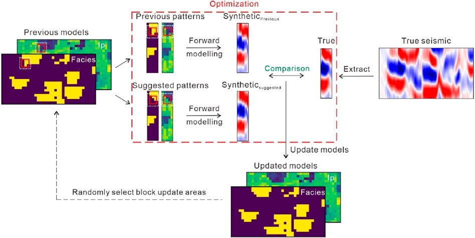
Figure 1. Block updating resample iterative geostatistical seismic inversion.

2.3 Multiscale strategy

A multiscale strategy categorizes the geological domain into various levels or scales, each representing distinct geological features that span from large-scale to small-scale heterogeneities. The suitability of the grid scale depends on the vertical and horizontal accuracy of the seismic data and specific developmental requirements. For instance, a coarse grid size may align with or surpass the accuracy of the seismic data. The level of grid refinement should be chosen based on the specific developmental requirements. The maximum number of conditioning data in data template is constant, while the size of these templates varies across these scales. The primary advantage of the multiscale approach lies in its ability to explore large-scale structures without restoring a large number of conditioning data points. For examples, Figure 2 shows the second scale grids, two facie types are simulated, and three facie patterns are scanned from the training image using a large re-scaled 3 × 3 template, generating associated 6 × 6 patterns (red, green, and blue boxes in Figure 2). In this example, we considered the multiscale strategy as a coarsening scheme, which employs evenly spaced grids rather than a cardinal one.

Figure 2

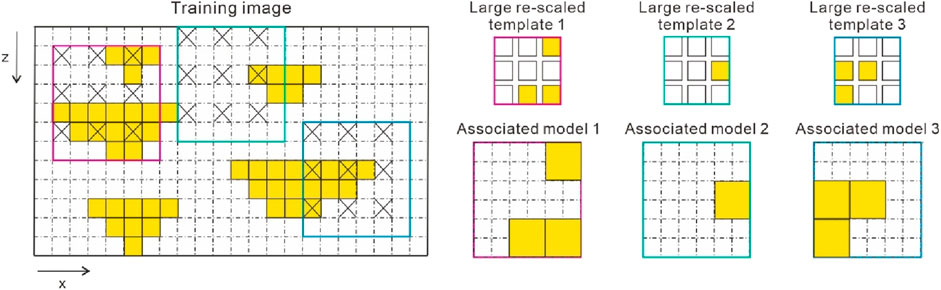
Figure 2. The skeletal of the multiscale strategy. Take the second scale grid, for example. Yellow and white grid cells represent sand and shale, respectively. The cells indicated with × in the training image are extracted patterns, forming the type of large re-scaled 3 × 3 data templates and associated models.

In the context of multiscale geostatistical seismic inversion, establishing a correspondence between time-domain seismic sampling points and depth-domain models is importance. On one hand, when the resolution of the simulated model exceeds that of the seismic data, we have the option to refine the simulation grid to align with the seismic sampling points (e.g., the third scale in Figure 3). Alternatively, we can reduce the sampling points of seismic wavelet and seismic records. On the other hand, geostatistical modelling can produce high-resolution models, primarily depending on the resolution of the training image and well-log data. However, the resolution of the inverted model, based on seismic inversion, is limited by the quality of seismic data (Figure 3). Thus, geostatistical modelling models at the small-scale grid, below the seismic resolution, necessitates either spaced sampling or coarsening for convolution with seismic wavelets to compute synthetic seismic records. These synthetic records are subsequently matched to observed low-resolution seismic data (e.g., first scale in Figure 3).

Figure 3

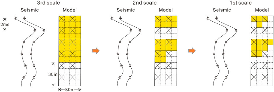
Figure 3. Correspondence between seismic sampling points and simulated cells at different-scale grids. The seismic sampling interval is 2 ms (around 15 m). The spacing between seismic traces is 15 m.

2.4 Proposed smoothed multiscale strategy

In the block updating process, the suggested patterns are suggested and then decide whether to replace it with the existing patterns (the red dotted lines in Figure 1). To achieve more comprehensive exploration of the prior space at the coarsest grid level and to enhance the likelihood of preserving previous models during the transition between two scale grids, this paper introduces a novel smoothed multiscale strategy for iterative geostatistical seismic inversion (SmoGSI). This strategy comprises two key components: a simulated annealing (SA) method for the smooth search the best coarsest model at the coarsest scale and a smooth transition (ST) method to convert a coarse model into a fine model (Figure 4). The detailed procedure of SmoGSI is descript in Algorithm 1.

Figure 4

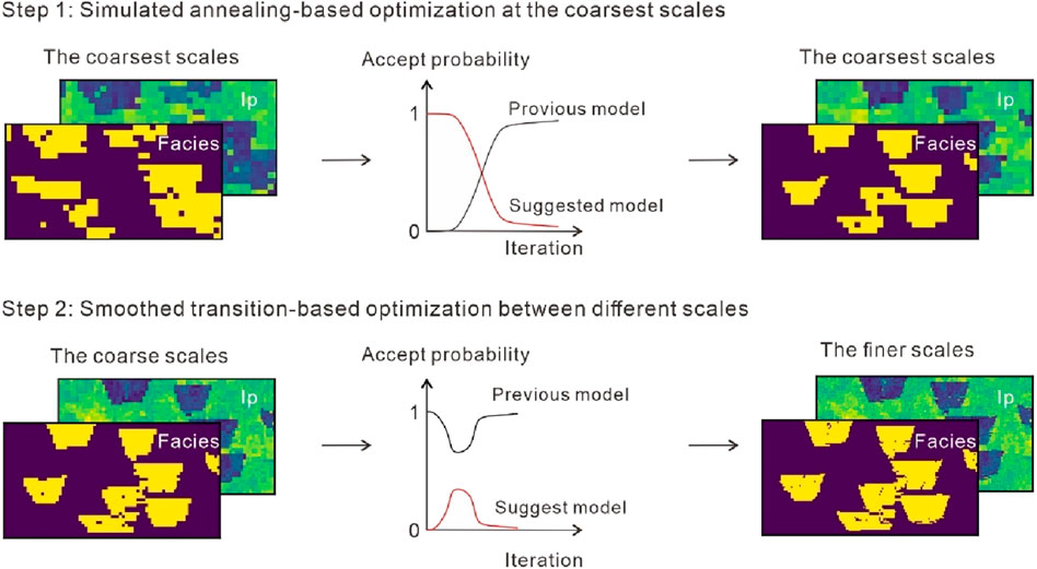
Figure 4. The smoothed multiscale strategy in the SmoGSI.

During the inversion of the coarsest-scale grids, the SA method is used to explore the prior space and find the most suitable large structures. This prevents the generated models from becoming trapping in local minimal. In this phase, we significantly reduce the number of model parameters. For example, in the third-scale grids, we only use one-sixteenth of the parameters. Equation 3 defined the acceptance rate for the suggested model:

$\alpha \left(m^k,m^{k+1}\right)=\min \left\{1,|\exp |\left(-\frac{L_{k+1}-L_k}{{\beta T}^k}\right)\right\}(3)$

where $T$ is the temperature in the current iteration, $\mathrm{\alpha }$ is the acceptance probability for the proposed model $m^{k+1}$ which replaces the previous model $m^k$, $L_k$ and $L_{k+1}$ are the likelihood functions obtained at the iteration $k$ and $k+1$. $T^{k+1}={\beta T}^k$, and $T^k$ is the annealing temperature at iteration $k$. As the temperature is sufficiently high, we will scan the prior solution space broadly; As the temperature decreases, the likelihood of accepting inferior suggested models diminishes; As the temperature approaches zero, only high-quality suggested models are accepted.

In the conversion from the coarse model to the fine model, using the SA temperature variation scheme may be not suitable for the fine grid models. High temperatures can disrupt the structure of “the best model” constructed at the coarsest grid level. Typically, the reduction in grid level leads to an increase in the mean accepted rate for the suggested models (AR) from Hu’s work (Hu et al., 2023). AR is defined as the ratio of accepted proposals to the total number of proposals made after a certain number of iterations (e.g., per 100 iterations). Inspired by linear combinations of variogram models (Azevedo and Soares, 2017) and the smooth transition methods (Karras et al., 2017), Here, we apply a similar method, the smoothed conversation method, to avoid the damage of the coarser structures in multiscale iterative geostatistical seismic inversion. Thus, rather than selecting the better model based on the comparison of the fitting of synthetic and observed seismic data, we enable the inverted models to transition smoothly from low-resolution models to high-resolution models. During this transition between different scales, Equation 4 defined the acceptance rate for the suggested model:

$\mathrm{\alpha }\left({\mathrm{m}}^{\mathrm{k}},{\mathrm{m}}^{\mathrm{k}+1}\right)=\left\{\begin{array}{c}1,\gamma L_{k+1}\le \left(1-\gamma \right)L_k\\ 0,\gamma L_{k+1}>\left(1-\gamma \right)L_k\end{array}\right.(4)$

where $\gamma$ is the smoothing factor, starting at 0 and incrementally increase (e.g., 0.1, 0.2, …, 0.4, up to 0.5). Thus, previous models are retained with high probability (i.e., close to 1) in situations where large structures are more likely to be retained and transition to normal probability (i.e., decided by the objected function) in cases where better patterns are more probable.

Algorithm 1.SmoGSI.

Input: Well data, observed seismic data, training image, wavelets

  1. Generate initial coarsest models

  for i = 1, …, 400 do

    2. Suggest facies and Ip patterns;

    3. Evaluate the objective function of the        suggested and previous models;

    if at the coarsest scales (e.g., i $\le$ 200)

      4. Use the acceptance rate in Equation 3 to          accept the suggested models;

      5. Cool the temperature

    else if (e.g., i $>$ 200)

      6. Use the acceptance rate in Equation 4 to          accept the suggested model;

      7. Increase the smoothing factors;

    end if

  end for

Output: Inverted facies and Ip models

3 Application examples

In this section, we evaluate SmoGSI, a novel iterative geostatistical seismic inversion method, using two datasets: a synthetic dataset from the Stanford Center for Reservoir Forecasting (SCRF) and a real dataset from the Dagang oilfield in China. We conduct a comparative analysis by pitting SmoGSI against a slightly modified version of González’s method (hereinafter referred to GSI), focusing on variation in SA and ST strategies.

3.1 Synthetic examples application

Figure 5 displays a reference section of sinuous channels from the Stanford VI-E reservoirs, which spans 80 m in thickness and 3,750 m in Common Depth Point (CDP) coordinate, comprising 150 × 80 grid cells. Specifically, Figures 5A–C show the reference facies, acoustic impedance (Ip), and noise-free full-stack seismic data, respectively, with well locations indicated at CDPs 40 and 120. The training image comprises four randomly selected sections from the Stanford VI-E reservoirs, twice the size of the simulated area (Figure 5D). Detailed input parameters for SmoGSI are provided in Table 1.

Figure 5

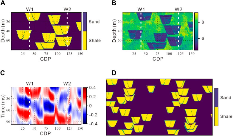
Figure 5. (A) Reference lithofacies. (B) $I_P$. (C) Seismic data. (D) The training image.

Table 1

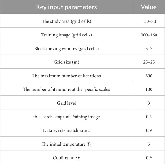
Table 1. The input parameters for SmoGSI.

GSI was employed for reference. The primary modification involves the multiscale strategy and the number of suggested patterns (facies and elastic parameters) samples per iteration. Unlike González’s original method, which performs multigrid operations at each iteration (from large-scale to small-scale), GSI progressively reduces grid levels throughout iterations. In other words, after simulating small-scale structures, large-scale structures are not simulated. Additionally, GSI considers only a single group of suggested patterns in each block update, as opposed to several groups in González’s original method. This alteration facilitates a more direct comparison with SmoGSI. To analyze the effects of SA and ST strategies during the iterative process, we integrate them separately with GSI, resulting in two methods: SA-GSI and ST-GSI. After extensive experimentation, we set the initial temperature for SA to 5 (a moderate value) to avoid prolonged high temperatures that will hinder convergence speed. The initial smoothing factor for ST is set to 0.45 to avoid prolonged low smoothing factors that could impede model updates.

Figure 6 shows the average curves from 20 runs of four methods: GSI, SA-GSI, ST-GSI, and SmoGSI. These methods progress through three stages: Third-scale grids (iteration <200), second-scale grids (200 < iteration < 300), and first-scale grids (iteration >300). The reduction in grid levels results in smaller residual errors between the model and seismic data, signifying that grid refinement enhances data fitting. Ultimately, all methods converge to low residuals (<300) with GSI exhibits the largest residuals. SA aids in the initial broad exploration of the prior parameter space (0.5 < AR < 1) in the coarsest scale grid, gradually favoring better-suggested models, leading to smaller residuals compared to the method without SA. Similarly, ST assists the inversion in capturing previous coarse structures initially, followed by gradually accepting suggested finer structures, leading to smaller residuals compared to the method without ST. Consequently, SmoGSI, combining SA and ST at different scales, exhibits smoother residual curves than GSI, resulting in a more effective fit with the seismic data.

Figure 6

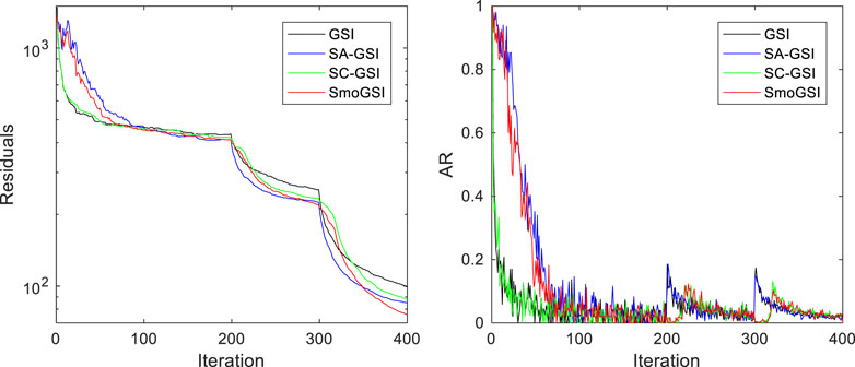
Figure 6. The residuals and AR of the GSI, SA-GSI, ST-GSI, and proposed SmoGSI.

Figures 7, 8 show inverted facies models and Multidimensional Scaling (MDS) plots for the four methods during the inversion process. Initially, the facies distribution is random in the first iteration, as realizations are generated without considering seismic data conditioning (Figure 7). Methods with SA (SA-GSI and SmoGSI) exhibit superior facies distribution by iteration 200 (Figure 7), with broader scatter distribution at the coarsest-scale grid (Figure 8A). In contrast, methods without SA become trapped in local minima at the coarsest-scale grid, resulting in unrealistic facies model (e.g., red circle in ST-GSI facies realizations in Figure 7). Methods lacking ST tends to lose large-scale structures (e.g., white circle in SA-GSI facies realizations in Figure 7). In Figure 8, Euclidean distance between the reference facies model and inverted facies models from the four methods are computed. The shorter the distance between two data, the higher the similarity between their facies models. We consider the first two dimensions of the MDS space, explaining approximately 70% of the data variance (Figure 8B). The scattered points, transitioning from light to dark colors, represent the optimization process of the inversion (i.e., the light color indicates the initial result, while the dark color represents the optimized result), with ST contributing to a smoother optimization process (indicated by red and green points in Figure 8A) compared to methods without ST (indicated by orange and blue points in Figure 8A). SmoGSI yields the best results since the distance between SmoGSI and the reference data is the shortest.

Figure 7

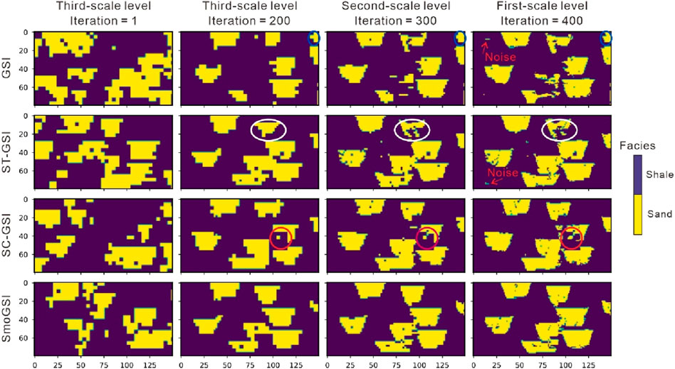
Figure 7. The inverted facie results of the four methods.

Figure 8

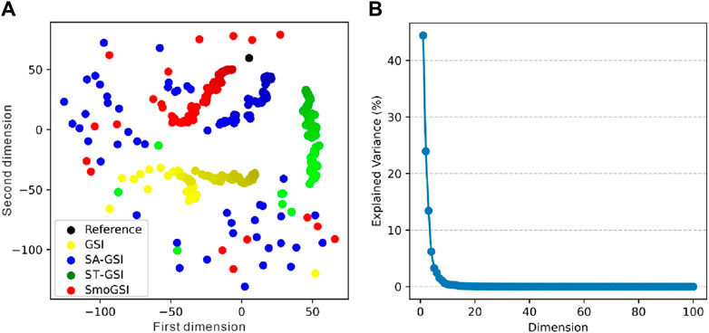
Figure 8. (A) The reference and inverted facie models in the MDS. (B) Explained variance by dimension.

Figure 9 displays the average Ip models resulting from 20 groups of realizations for each of the four methods. Each group of realizations represents the last optimal model after 400 iterations of iterative geostatistical seismic inversion. These models closely resemble the associated reference models, with SmoGSI exhibiting lower mean Ip model uncertainty compared to the other three methods. This result can be attributed to the superior facies models generated by SmoGSI, which constraint samples of elastic properties. Furthermore, when comparing the difference between the theoretical and simulated Ip models, GSI exhibits the largest difference, while SmoGSI shows the smallest difference. This same effect is observed in the best-fit realization of Ip obtained from the 20 groups of realizations (Figure 10). The curve results from SmoGSI closely match the reference models, indicating that SmoGSI’s outcomes better produce the probability distribution of Ip.

Figure 9

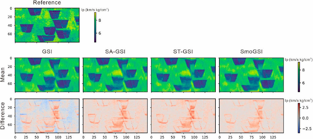
Figure 9. The difference in Ip of the GSI, SA-GSI, ST-GSI, and SmoGSI.

Figure 10

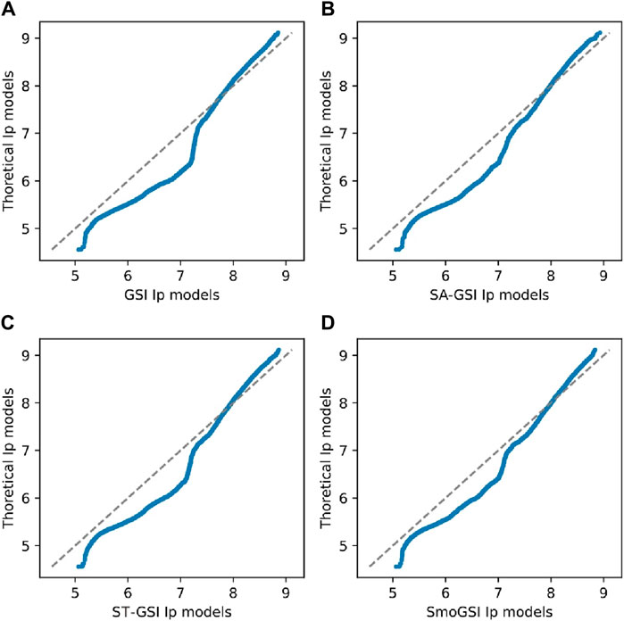
Figure 10. Q-Q plot of four methods: (A) GSI Ip models; (B) SA-GSI Ip models; (C) ST-GSI Ip models; (D) SmoGSI Ip models.

The synthetic records in Figure 11 are generated from the mean Ip models. All four sets of results closely resemble the reference seismic data. When comparing the average correlation coefficients between the reference and synthetic record traces, it is observed that the average correlation coefficient from GSI is approximately 0.95, while those from the other methods hover around 0.97. SmoGSI attains the highest correlation coefficient, underscoring its superior performance (Figure 12).

Figure 11

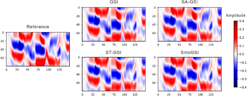
Figure 11. Seismic data from the mean Ip model of four methods.

Figure 12

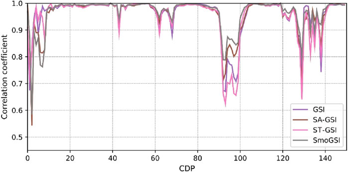
Figure 12. Trace-by-trace correlation from four methods.

3.2 Real examples application

We applied GSI and SmoGSI to real datasets obtained from the Dagang oilfield in China, where a meandering river sedimentary environment had developed. The inversion grid consists of 370 × 100 grid cells in the x- and z-directions, respectively, with a grid size of 20 m × 1.2 m. Figure 13 displays the location of two available vertical wells. Figure 14A shows the wavelet, while Figure 14B shows the Ip-well log obtained from two wells.

Figure 13

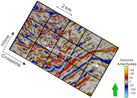
Figure 13. Seismic grid and location of well. The white line is the vertical well section which will be inverted.

Figure 14

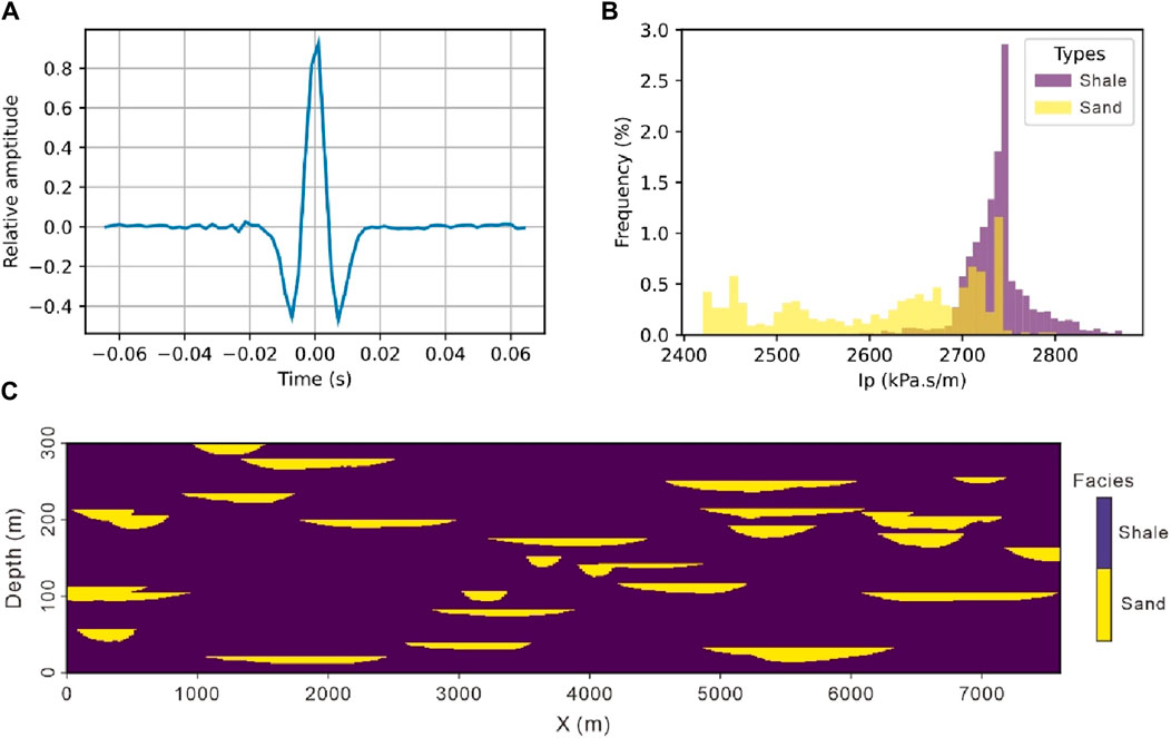
Figure 14. (A) Wavelet, (B) Ip-log data, and (C) The training image.

We utilized an objected-based method on the Petrel software to simulate a representative training image of the sand-shale channel system. The simulation referenced geometric parameters of the channels derived from both well (e.g., channel depth parameters) and seismic data (e.g., channel width parameters). The training images encompass a wide range of channel widths and depths, providing a broader prior space that includes the statistical range of channel parameters from well and seismic data. The channels in the training dataset have a length equivalent to that of the inverted section and a width twice its length, represented as 370 × 200 grid cells (Figure 14C).

We adopted the correlation coefficient as the objective function for this application. Seismic data were sampled at a rate of 2 ms, with 100 ms intervals for inversion. The vertical grid cell size was set to 1 ms (approximately 1.2 m), smaller than the vertical resolution of seismic data. We retained the horizontal grid cell size consistent with the horizontal resolution of the seismic data, which remained at 20 m.

The inversion process comprised a total of 400 iterations. A higher number of iterations (200 times) were allocated to the coarsest scale grids to rapidly generate preliminary channel distributions. In contract, at finer scale grids, we optimized the model with a reduced number of iterations (100 times in both the second and first scale grids) due to the increased time required for simulations with finer grids. After thorough experimentation, we fine-tuned the initial smoothing factor in ST to 0.49, a value very close to 0.5, with an incremental increase of 0.0002 per iteration. This adjustment aimed to prevent prolonged periods of low-smoothing factors from impeding model updates, especially considering the minor changes in the objective function during the update process.

Figures 15–17 display the best-fit facies, Ip, and synthetic records generated using both GSI and SmoGSI. Due to the substantial distance between well W1 and W2, we relied on facies pattern guidance from the training image and response characteristics from the seismic data to determine facies distributions between the two wells. The fidelity of large-scale and small-scale facies patterns reproduction served as a reflection of the modelling capabilities of different multiscale strategies. In comparison to the GSI facies results, SmoGSI exhibited superior noise suppression both between and within channels, with improved channel contours, including isolated channels and vertically stacked channels (red dotted lines in Figure 15). The distribution of Ip properties in both inversion methods was constrained by the facies distribution, taking into account the statistical relationship between facies and Ip. Areas with sand distribution displayed lower Ip value, while areas with mudstone distribution exhibited higher Ip value (Figure 16). Since SmoGSI benefited from its superior guidance of large-scale and small-scale facies patterns, the associated Ip properties by its inversion also have better channel contours and also consistent with the well-log data. For example, in the SmoGSI Ip model, the low Ip position of W1 corresponded to three channels (red dotted lines in Figure 16). Comparing actual and synthetic seismic data in terms of relative amplitude, Figure 17 that both synthetic records closely resembled actual seismic data.

Figure 15

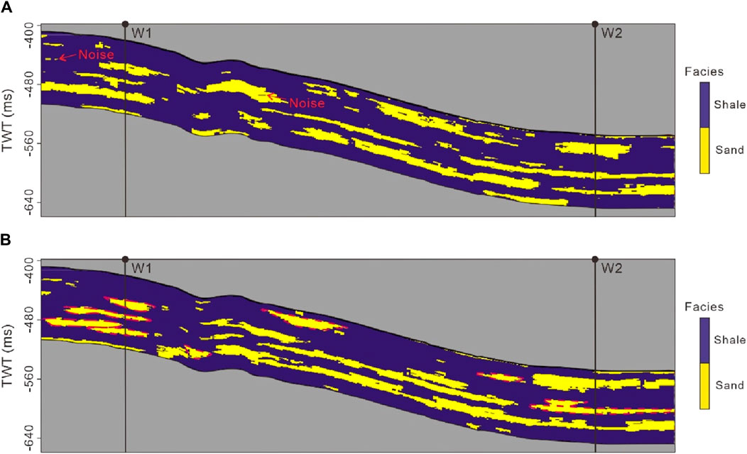
Figure 15. Facies models from (A) GSI and (B) SmoGSI.

Figure 16

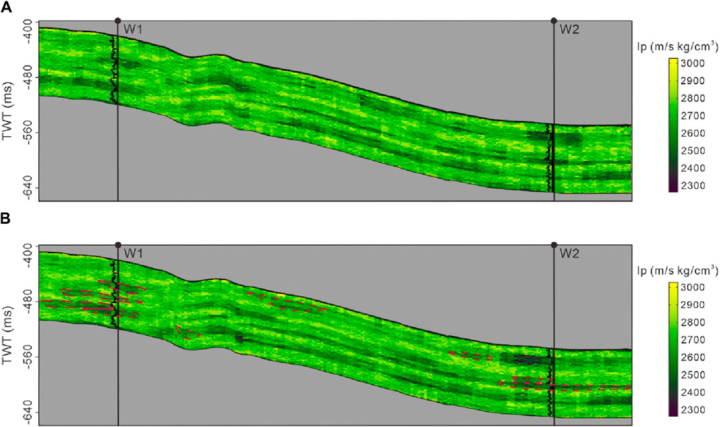
Figure 16. Ip models from (A) GSI and (B) SmoGSI.

Figure 17

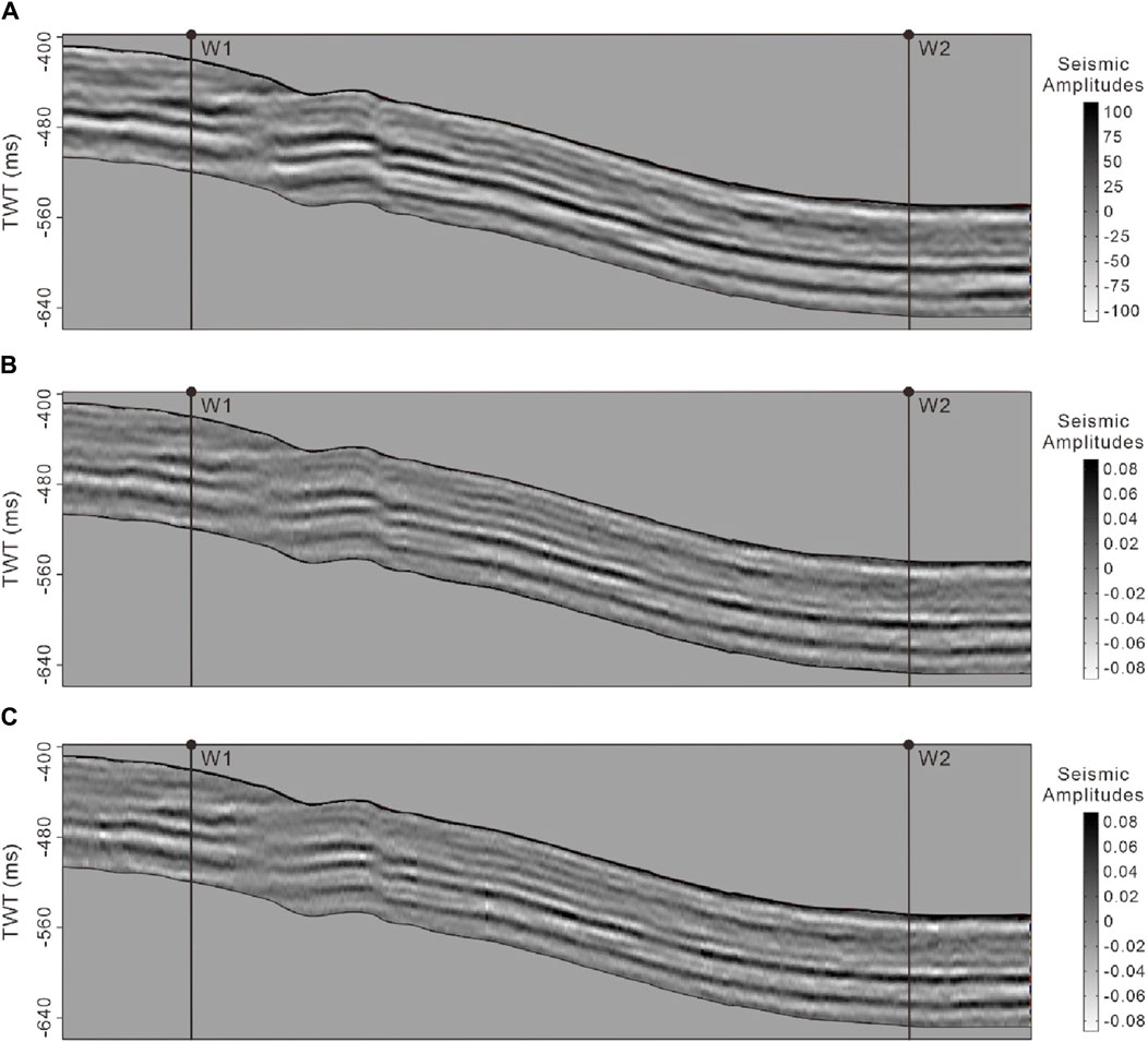
Figure 17. (A) Actual seismic data. (B) Synthetic seismic records from GSI. (C) Synthetic seismic records from SmoGSI.

Figure 18 presents the variation in correlation coefficient and AR resulting from the GSI and SmoGSI inversion methods. Notably, the SmoGSI outperformed GSI in terms of AR. In summary, these results demonstrate the effectiveness of SmoGSI when applied to real datasets, yielding good results.

Figure 18

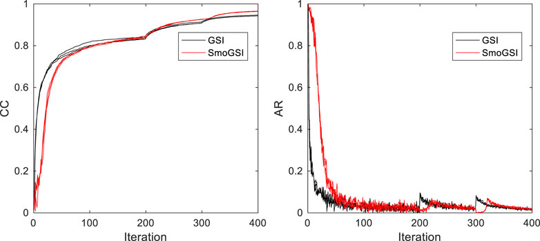
Figure 18. The correlation coefficient and AR from GSI and SmoGSI.

4 Discussion

The proposed method employs simulated annealing and smoothed transition techniques as the model perturbation methods at different scales within iterative geostatistical seismic inversion. Specifically, at coarsest-scales level, we favor accept perturbations to explore the inversion solution space, while at finer-scale level, the preference shifts toward rejecting perturbations to preserve existing large-scale structural features.

In the SA strategy, two key parameters come into play: the initial temperature and cooling factor. The time cost of large-scale grid iteration is relatively small compared to small-scale grid iteration. Although setting a very high temperature (e.g., 10⁵) and a high cooling factor (e.g., 0.999) can improve the search for the global optimum in inversion results, such parameters tend to slow down the optimization process. Similarly, in the ST strategy, two key parameters are involved: the smoothing factor and its increment. Opting for a very low smoothing factor (e.g., 0) and a low factor increment (e.g., 10^−-5) can help the inversion maintain the existing large-scale structures, but it is also results in a slower optimization process. Consequently, the challenge lies in finding a balance between time cost and achieve the optimal solution when selecting appropriate parameters for SA and ST. Additionally, SA is relatively simple to implement and can be easily adapted to various types of optimization problems due to its flexibility in dealing with different types of objective functions. Other global optimization algorithms, such as the genetic algorithm and quantum annealing algorithm, which are suitable for finding optimal patterns can be potential substitutes for SA.

We focus on a new smoothed multiscale strategy to improve the overall accuracy of the subsurface property estimations, and thus, we discuss modelling time less extensively. For the computational efficiency in geological modelling, alternative algorithm such as DS (Mariethoz et al., 2010) can speed up the modelling process compared to SIMPAT (Arpat, 2005). It worth noting that the pixel-based geostatistical technique (e.g., DS) pairs well with point updates iterative process, while the patch-based geostatistical technique (e.g., SIMPAT) is compatible with block updates iterative process. Furthermore, implementing the MPS algorithm with parallel computation would also benefit our approach by reducing time costs.

The proposed method relies on post-stack data and P-wave impedance for lithology recognition. However, when the impedances of sand and mudstone overlap significantly, as in tight sandstone formations, distinguishing between these lithologies using P-wave impedance alone can be challenging. To address this issue, additional techniques and data can be integrated to improve lithology differentiation. For instance, combining P-wave impedance with other geophysical measurements, such as S-wave impedance or other seismic attributes, can enhance the discrimination between sand and mudstone.

The introduction of the smoothed multiscale strategy present exciting opportunities in the field of geostatistical seismic inversion. By improving the transition between scales and optimizing models, this approach has the potential to provide more accurate estimations of subsurface properties while simultaneously reducing noise in simulated areas. Future research may explore the application of this strategy across various geological and geophysical contexts.

5 Conclusion

This paper introduces the smoothed multiscale iterative geostatistical seismic inversion (SmoGSI) method, which offer a robust solution for enhancing the precision and reliability of subsurface property estimations through seamlessly transitions between coarse and fine-scale models. The comprehensive assessment of SmoGSI using synthetic and real case studies, demonstrates its superior performance. SmoGSI consistently outperforms existing multiscale iterative geostatistical seismic inversion methods in terms of convergence speed, facies modelling, and correlation coefficients with reference seismic data.

Data availability statement

The original contributions presented in the study are included in the article/supplementary material, further inquiries can be directed to the corresponding authors.

Author contributions

QK: Methodology, Writing–original draft, Writing–review and editing. JH: Conceptualization, Funding acquisition, Supervision, Writing–review and editing. XH: Methodology, Validation, Writing–review and editing. YL: Supervision, Writing–review and editing. QR: Validation, Writing–review and editing. MH: Writing–review and editing. YY: Supervision, Writing–review and editing.

Funding

The authors declare that financial support was received for the research, authorship, and/or publication of this article. This work was supported by the National Natural Science Foundation of China (No. 42072146).

Acknowledgments

We gratefully acknowledge the support of Leonardo Azevedo at CERENA, Instituto Superior Ténico, Universidade de Lisboa.

Conflict of interest

Author QR was employed by SINOPEC Geophysical Research Institute Co., Ltd. Author MH was employed by Research Institute of Petroleum Exploration and Development (PetroChina).

The remaining authors declare that the research was conducted in the absence of any commercial or financial relationships that could be construed as a potential conflict of interest.

Publisher’s note

All claims expressed in this article are solely those of the authors and do not necessarily represent those of their affiliated organizations, or those of the publisher, the editors and the reviewers. Any product that may be evaluated in this article, or claim that may be made by its manufacturer, is not guaranteed or endorsed by the publisher.

References

Alcolea, A., and Renard, P. (2010). Blocking moving window algorithm: conditioning multiple-point simulations to hydrogeological data. Water Resour. Res. 46, W08511. doi:10.1029/2009WR007943

CrossRef Full Text | Google Scholar

Arpat, G. B. (2005). Sequential simulation with patterns. Ph.D. dissertation. Stanford: Stanford University.

Google Scholar

Azevedo, L. (2022). Model reduction in geostatistical seismic inversion with functional data analysis. Geophysics 87, M1–M11. doi:10.1190/geo2021-0096.1

CrossRef Full Text | Google Scholar

Azevedo, L., Narciso, J., Nunes, R., and Soares, A. (2021). Geostatistical seismic inversion with self-updating of local probability distributions. Math. Geosci. 53, 1073–1093. doi:10.1007/s11004-020-09896-9

CrossRef Full Text | Google Scholar

Azevedo, L., and Soares, A. (2017). Geostatistical methods for reservoir geophysics. Berlin: Springer International Publishing. doi:10.1007/978-3-319-53201-1

CrossRef Full Text | Google Scholar

Buland, A., and Omre, H. (2003). Bayesian linearized AVO inversion. Geophysics 68, 185–198. doi:10.1190/1.1543206

CrossRef Full Text | Google Scholar

Deutsch, C. V., and Journel, A. G. (1992). GSLIB: geostatistical software library and user's guide. Oxford: Oxford University Press.

Google Scholar

Doyen, P. (2007). Seismic reservoir characterization: an earth modelling perspective. EAGE. doi:10.3997/9789073781771

CrossRef Full Text | Google Scholar

Ferreirinha, T., Nunes, R., Azevedo, L., Soares, A., Pratas, F., Tomás, P., et al. (2015). Acceleration of stochastic seismic inversion in OpenCL-based heterogeneous platforms. Comput. Geosci. 78, 26–36. doi:10.1016/j.cageo.2015.02.005

CrossRef Full Text | Google Scholar

Fu, J., Caers, J., and Tchelepi, H. A. (2011). A multiscale method for subsurface inverse modeling: single-phase transient flow. Adv. Water Resour. 34, 967–979. doi:10.1016/j.advwatres.2011.05.001

CrossRef Full Text | Google Scholar

Fu, J., and Gómez-Hernández, J. J. (2008). A blocking Markov chain Monte Carlo method for inverse stochastic hydrogeological modeling. Math. Geosci. 41, 105–128. doi:10.1007/s11004-008-9206-0

CrossRef Full Text | Google Scholar

Gardet, C., Le Ravalec, M., and Gloaguen, E. (2014). Multiscale parameterization of petrophysical properties for efficient history-matching. Math. Geosci. 46, 315–336. doi:10.1007/s11004-013-9480-3

CrossRef Full Text | Google Scholar

González, E. F., Mukerji, T., and Mavko, G. (2008). Seismic inversion combining rock physics and multiple-point geostatistics. Geophysics 73, R11–R21. doi:10.1190/1.2803748

CrossRef Full Text | Google Scholar

Grana, D., de Figueiredo, L. P., and Azevedo, L. (2019). Uncertainty quantification in Bayesian inverse problems with model and data dimension reduction. Geophysics 84, 1–59. doi:10.1190/geo2019-0222.1

CrossRef Full Text | Google Scholar

Grana, D., Mukerji, T., Dvorkin, J., and Mavko, G. (2012). Stochastic inversion of facies from seismic data based on sequential simulations and probability perturbation method. Geophysics 77, 53–M72. doi:10.1190/geo2011-0417.1

CrossRef Full Text | Google Scholar

Hansen, T. M., Cordua, K. S., and Mosegaard, K. (2012). Inverse problems with non-trivial priors: efficient solution through sequential Gibbs sampling. Comput. Geosci. 16, 593–611. doi:10.1007/s10596-011-9271-1

CrossRef Full Text | Google Scholar

Hu, X., Hou, J., Yin, Y., Liu, Y., Wang, L., Kang, Q., et al. (2023). A multi-scale blocking moving window algorithm for geostatistical seismic inversion. Comput. Geosci. 173, 105313. doi:10.1016/j.cageo.2023.105313

CrossRef Full Text | Google Scholar

Hu, X., Song, S., Hou, J., Yin, Y., Hou, M., and Azevedo, L. (2024). Stochastic modeling of thin mud drapes inside point bar reservoirs with ALLUVSIM-GANSim. Water Resour. Res. 60, e2023WR035989. doi:10.1029/2023WR035989

CrossRef Full Text | Google Scholar

Karras, T., Aila, T., Laine, S., and Lehtinen, J. (2017). Progressive growing of GANs for improved quality, stability, and variation. ArXiv Prepr. arXiv: 1710.10196. doi:10.48550/arXiv.1710.10196

CrossRef Full Text | Google Scholar

Laloy, E., Linde, N., Jacques, D., and Mariethoz, G. (2016). Merging parallel tempering with sequential geostatistical resampling for improved posterior exploration of high-dimensional subsurface categorical fields. Adv. Water Resour. 90, 57–69. doi:10.1016/j.advwatres.2016.02.008

CrossRef Full Text | Google Scholar

Liu, M., and Grana, D. (2019). Accelerating geostatistical seismic inversion using TensorFlow: a heterogeneous distributed deep learning framework. Comput. Geosciences 124, 37–45. doi:10.1016/j.cageo.2018.12.007

CrossRef Full Text | Google Scholar

Liu, X., Chen, X., Cheng, J., Zhou, L., Chen, L., Li, C., et al. (2023). Simulation of complex geological architectures based on multistage generative adversarial networks integrating with attention mechanism and spectral normalization. IEEE Trans. Geoscience Remote Sens. 61, 1–15. doi:10.1109/TGRS.2023.3294493

CrossRef Full Text | Google Scholar

Liu, X., Li, J., Chen, X., Guo, K., Li, C., Zhou, L., et al. (2018). Stochastic inversion of facies and reservoir properties based on multi-point geostatistics. J. Geophys. Eng. 15, 2455–2468. doi:10.1088/1742-2140/aac694

CrossRef Full Text | Google Scholar

Liu, Y. (2006). Using the Snesim program for multiple-point statistical simulation. Comput. Geosciences 32, 1544–1563. doi:10.1016/j.cageo.2006.02.008

CrossRef Full Text | Google Scholar

Mariethoz, G. (2010). A general parallelization strategy for random path based geostatistical simulation methods. Comput. Geosciences 36, 953–958. doi:10.1016/j.cageo.2009.11.001

CrossRef Full Text | Google Scholar

Mariethoz, G., Renard, P., and Caere, J. (2010a). Bayesian inverse problem and optimization with iterative spatial resampling. Water Resour. Res. 46, 2387–2392. doi:10.1029/2010WR009274

CrossRef Full Text | Google Scholar

Mariethoz, G., Renard, P., and Straubhaar, J. (2010b). The Direct Sampling method to perform multiple-point geostatistical simulations. Water Resour. Res. 46. doi:10.1029/2008WR007621

CrossRef Full Text | Google Scholar

Nunes, R., Azevedo, L., and Soares, A. (2019). Fast geostatistical seismic inversion coupling machine learning and Fourier decomposition. Comput. Geosci. 23, 1161–1172. doi:10.1007/s10596-019-09877-w

CrossRef Full Text | Google Scholar

Pereira, Â., Azevedo, L., and Soares, A. (2023). Updating local anisotropies with template matching during geostatistical seismic inversion. Math. Geosci. 55, 497–519. doi:10.1007/s11004-023-10051-3

CrossRef Full Text | Google Scholar

Shi, Y., Yu, B., Zhou, H., Cao, Y., Wang, W., and Wang, N. (2024). FMG_INV, a fast multi-Gaussian inversion method integrating well-log and seismic data. IEEE Trans. Geoscience Remote Sens. 62, 1–12. doi:10.1109/TGRS.2024.3351207

CrossRef Full Text | Google Scholar

Song, S., Mukerji, T., and Hou, J. (2021). Geological facies modeling based on progressive growing of Generative Adversarial Networks (GANs). Comput. Geosci. 25, 1251–1273. doi:10.1007/s10596-021-10059-w

CrossRef Full Text | Google Scholar

Tran, T. T. (1994). Improving variogram reproduction on dense simulation grids. Comput. Geosciences 20, 1161–1168. doi:10.1016/0098-3004(94)90069-8

CrossRef Full Text | Google Scholar

Wang, Z., Chen, T., Hu, X., Wang, L., and Yin, Y. (2022). A multi-point geostatistical seismic inversion method based on local probability updating of lithofacies. Energies 15, 299. doi:10.3390/en15010299

CrossRef Full Text | Google Scholar

Yang, L., Hou, W., Cui, C., and Cui, J. (2016). GOSIM: a multi-scale iterative multiple-point statistics algorithm with global optimization. Comput. Geosciences 89, 57–70. doi:10.1016/j.cageo.2015.12.020

CrossRef Full Text | Google Scholar

Yu, B., Shi, Y., Zhou, H., Cao, Y., Wang, N., and Ji, X. (2024). Fast Bayesian linearized inversion with an efficient dimension reduction strategy. IEEE Trans. Geoscience Remote Sens. 62, 1–10. doi:10.1109/TGRS.2024.3360031

CrossRef Full Text | Google Scholar

Zhang, T., Yang, Z., and Sun, C. (2022). Stochastic simulation of fan deltas using parallel multi-stage generative adversarial networks. J. Petroleum Sci. Eng. 208, 109442. doi:10.1016/j.petrol.2021.109442

CrossRef Full Text | Google Scholar