Slope deformation prediction based on noise reduction and deep learning: a point prediction and probability analysis method

Slope deformation, a key factor affecting slope stability, has complexity and uncertainty. It is crucial for early warning of slope instability disasters to master the future development law of slope deformation. In this paper, a model for point prediction and probability analysis of slope deformation based on DeepAR deep learning algorithm is proposed. In addition, considering the noise problem of slope measurement data, a Gaussian-filter (GF) algorithm is used to reduce the noise of the data, and the final prediction model is the hybrid GF-DeepAR model. Firstly, the noise reduction effect of the GF algorithm is analyzed relying on two actual slope engineering cases, and the DeepAR point prediction based on the original data is also compared with the GF-DeepAR prediction based on the noise reduction data. Secondly, to verify the point prediction performance of the proposed model, it is compared with three typical point prediction models, namely, GF-LSTM, GF-XGBoost, and GF-SVR. Finally, a probability analysis framework for slope deformation is proposed based on the DeepAR algorithm characteristics, and the probability prediction performance of the GF-DeepAR model is compared with that of the GF-GPR and GF-LSTMQR models to further validate the superiority of the GF-DeepAR model. The results of the study show that: 1) The best noise reduction is achieved at the C1 and D2 sites with a standard deviation σ of 0.5. The corresponding SNR and MSE values are 34.91 (0.030) and 35.62 (0.674), respectively. 2) A comparison before and after noise reduction reveals that the R² values for the C1 and D2 measurement points increased by 0.081 and 0.070, respectively. Additionally, the MAE decreased from 0.079 to 0.639, and the MAPE decreased from 0.737% to 0.912%. 3) The prediction intervals constructed by the GF-DeepAR model can effectively envelop the actual slope deformation curves, and the PICP in both C1 and D1 is 100%. 4) Whether it is point prediction or probability prediction, the GF-DeepAR model excels at extracting feature information from slope deformation sequences characterized by randomness and complexity. It conducts predictions with high accuracy and reliability, indicating superior performance compared to other models. The results of the study can provide a reference for the theory of slope deformation prediction, and can also provide a reference for similar projects.

1 Introduction

The stability of slopes is crucial for engineering safety (Peng et al., 2019; Qiu et al., 2024). Influenced by a variety of environments, the originally stable slopes are prone to lose their original equilibrium under the action of external or internal stresses, which may lead to disasters such as landslides and collapses. For example, in September 2008, landslides occurred in Jintou Mountain in the southern part of the Taipei Basin, which greatly impacted the safety of the residential community in the downslope location (Nguyen et al., 2022). On 17 September 2011, a landslide occurred in Baqiao District, Shaanxi, China, which causing severe casualties in terms of people and property (Lin et al., 2017), and on 28 June 2016, a landslide occurred in Xinlu Village, Shuicheng, Chongqing (Zuo et al., 2022). Currently, advance identification and trend prediction of disasters is one of the most important means to avoid losses and casualties caused by slope disasters. Slope deformation, as a key factor affecting its stability, has complexity and uncertainty, and mastering its future development pattern is crucial for early warning of slope instability disasters.

In recent years, many intelligent prediction algorithms have been applied to slope deformation prediction (Deng et al., 2021). Initially, more applications are static models such as the Support Vector Machine Regression (SVR) algorithm (Xu et al., 2022), the Autoregressive Moving Average (ARMA) algorithm (Shen et al., 2018), and the Backpropagation (BP) algorithm (Zhang et al., 2023). Since 2006, Deep Learning has achieved great success in the field of machine learning (Lasantha et al., 2023). Deep learning-based recurrent neural network (RNN) models with deeper network structures and more powerful representation learning capabilities are particularly favored by researchers (Cao et al., 2023). Currently, RNN models have achieved more research results in the field of slope deformation prediction (Xie et al., 2019). Long Short-Term Memory (LSTM) is a kind of RNN, Xi et al. (2023) established an LSTM slope deformation model based on the time-series deformation data from seven on-site monitoring points of Huanglianshu landslide and found that the prediction accuracy was better. Wang et al. (2024) used the LSTM algorithm to predict and analyze the deformation data of complex road graben slopes and compared it with other kinds of prediction models, and found that the LSTM slope deformation prediction model proposed in this paper is more accurate. Zhang et al. (2024) proposed a slope deformation prediction method based on LSTM for the stability of loosely stacked body slopes and demonstrated that the method can be used as an effective measure to mitigate landslide losses. The above studies demonstrate the applicability of deep learning models in slope deformation prediction and promote the progress of research work in this field, but there are still several problems need to be optimized. Firstly, although the LSTM model is capable of capturing the long-term dependence of slope deformation, it is relatively weak in handling mutations or outliers (Zhu et al., 2024), leading to limitations in its prediction accuracy (Chen et al., 2019). Secondly, the monitoring data used to train the prediction model is easily affected by conditions such as monitoring equipment and field environment, leading to the problem of data noise (Dong et al., 2023). This in turn affects the quality of the dataset and leads to unsatisfactory prediction results. Thirdly, the prediction results obtained from the existing studies are all point prediction results, resulting in low credibility of the results, which in turn limits the value of popularization and application.

DeepAR algorithm is an improved algorithm based on RNN and LSTM (Salinas et al., 2020). The algorithm was first proposed by Salina et al., in 2017 (Schaduangrat et al., 2023). The DeepAR algorithm contains a recurrent neural network structure inside, which has the same memory and parameter sharing as LSTM (Singh et al., 2024). In addition, DeepAR can adjust the probability distribution by probability modeling, which allowing it to learn the inherent laws and patterns of the slope deformation sequence data, rather than just simple linear relationships or trends. Hence, the DeepAR algorithm is able to capture this change and flexibly adjust according to the previously learned patterns, thus provide more robust predictions (Chang and Jia, 2023), when there is a sudden change in the original data. Currently, the DeepAR algorithm has been successfully applied in the fields of healthcare (Schaduangrat et al., 2023), finance (Soliman et al., 2023), and environmental protection (Jiang et al., 2021), and can also provide an effective means for accurate and reliable prediction of slope deformation. In addition, the current slope engineering measurement data are susceptible to noise problems due to a variety of conditions, limiting the accuracy of slope deformation prediction (Ma et al., 2021). Including deep learning algorithms such as RNN, LSTM, DeepAR, etc., the above-mentioned algorithms are single prediction algorithms and cannot pre-process for the dataset before doing prediction analyses. Therefore, it is of great significance to propose a hybrid algorithm that guarantees the quality of prediction input data and provides prediction analyses based on established high-precision prediction algorithms.

To address the above issues, a model for prediction and probability analysis of slope deformation points based on GF and DeepAR algorithms is proposed. The structure of the paper is organized as follows: Section 2 provides a detailed introduction to the newly proposed method, which consists of three parts: filtering and noise reduction processing based on the GF algorithm, slope deformation prediction based on DeepAR, and point prediction performance assessment and comparison analysis. Section 3 shows the noise reduction results, prediction results, and comparison analysis results of the GF-DeepAR model on two real slope engineering cases. Section 4 proposes a probability analysis framework for slope deformation based on the GF-DeepAR model and compares the performance of other probability analysis models to further validate the superiority of the GF-DeepAR model. Section 5 concludes this work. Section 6 compares the study in this paper with existing similar studies, and also compares the prediction accuracy at different time steps, and finally discusses the future research outlook.

2 Hybrid GF-DeepAR prediction approach

2.1 DeepAR algorithm

DeepAR is a time series prediction method based on deep learning, which has a significant advantage in predicting the nonlinear features of the series and can well perform point prediction and probability prediction (Cao et al., 2023). The structure of the DeepAR model is shown in Figure 1. Define the value of the ith slope deformation sequence at the moment t as Z_i,t. The goal of the prediction model is to obtain the joint probability distribution $P\left(z_{i,t:T}\left|z_{i,t-1},\right.z_{i,1:T}\right)$ of the unknown sequence Z_i,t:T through the known slope deformation data Z_i,1:t-1 and covariates x_i,1:T. Assume that the distribution of the unknown slope deformation sequence is $Q_{\mathrm{\Theta }}\left(z_{i,t:T}\left|z_{i,t-1},\right.x_{i,1:T}\right)$, and its probability distribution as shown in Eq. 1:

$Q_{\mathrm{\Theta }}\left(z_{i,t:T}\left|z_{i,t-1},\right.x_{i,1:T}\right)={\displaystyle \prod _{t=t_0}^T}{Q}_{\mathrm{\Theta }}\left(z_{i,t}\left|z_{i,1:t-1},\right.x_{i,1:T}\right)(1)$

Figure 1

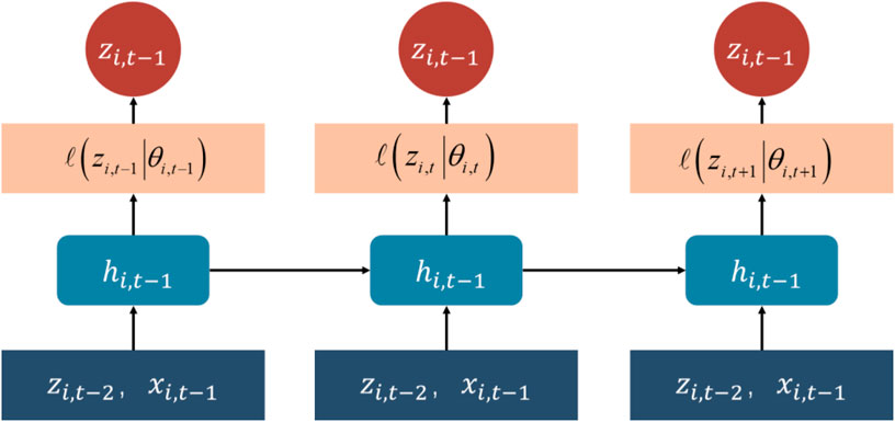
Figure 1. DeepAR network architecture.

And represent this distribution by a parametric likelihood function with, as shown in Eqs 2, 3:

${\displaystyle \prod _{t=t_0}^T}{Q}_{\mathrm{\Theta }}\left(z_{i,t}\left|z_{i,1:t-1},\right.x_{i,1:T}\right)={\displaystyle \prod _{t=t_0}^T}\mathcal{l}\left(z_{i,t}\left|\theta \left(h_{i,t},\mathrm{\Theta }\right)\right.\right)(2)$

$h_{i,t}=h\left(h_{i,t-1},z_{i,t-1},x_{i,t},\mathrm{\Theta }\right)(3)$

Where h is the implied state function of the RNN neural network, $\theta$ is the output state function, and $\mathrm{\Theta }$ is the network structure parameters.

It is worth noting that the model $\mathcal{l}\left(z\left|\theta \right.\right)$ should choose the likelihood function that best matches the statistical properties of the data, such as the Gaussian distribution likelihood function, the Bernoulli distribution likelihood function, and the negative binomial distribution likelihood function. Considering the characteristics of the data used in the study, Gaussian distribution is used as the likelihood model for slope deformation probability prediction, with the likelihood parameters $\theta =\left\{u,\sigma \right\}$, u as the expectation and $\sigma$ as the standard deviation. Each likelihood function has its corresponding activation function, in which to ensure that $\sigma$ is positive, the activation function of the output layer must be set as an exponential function (exponential activation function, softplus activation function), in this paper, we use the softplus as its activation function, as shown in Eq. 4:

$\mathcal{l}\left(z\left|u,\sigma \right.\right)=\frac{1}{\sqrt{2\pi {\sigma }^2}}\exp \left[\frac{-{\left(z-u\right)}^2}{2{\sigma }^2}\right](4)$

Where $\exp \left[\right]$ is a power function with e as the base.

2.2 GF algorithm

Gaussian-filter is a linear filtering technique with a probability density function obeying a normal distribution, which can be used to attenuate Gaussian noise interference in pit deformation data (Selva et al., 2020). The core idea of the Gaussian-filter algorithm is to iteratively convolve the original signal through the Gaussian kernel function, and use the weighted average of the neighborhood of a data point instead of that data point to obtain the filtered and noise-reduced signal.

Considering that the slope deformation data is a one-dimensional sequence, it is processed using a one-dimensional Gaussian function, as shown in Eq. 5:

$g\left(t,\sigma \right)=\frac{1}{\sqrt{2\pi }\sigma }\exp \left(-\frac{{\left(t-t_0\right)}^2}{2{\sigma }^2}\right)(5)$

Where: t is the sampling point for pit deformation monitoring, and t₀ is the mean value of t. Since the calculation takes the current sampling point as the origin, t₀ =0. Its first-order derivative $g^{\left(1\right)}\left(t,\sigma \right)$ is calculated as shown in Eq. 6:

$g^{\left(1\right)}\left(t,\sigma \right)=\frac{-t}{\sqrt{2\pi }{\sigma }^3}\exp \left(-\frac{t^2}{2{\sigma }^2}\right)(6)$

Where: $g^{\left(1\right)}\left(t,\sigma \right)$ is a Gaussian filter, and the slope deformation sequence function $f\left(t\right)$ is noise-reduced by $g^{\left(1\right)}\left(t,\sigma \right)$, further, S(t,σ) can be calculated as shown in Eq. 7:

$S\left(t,\sigma \right)=f\left(t\right)*g^{\left(1\right)}\left(t,\sigma \right)(7)$

Where: $\prime *\prime$ is the convolution operator; $\sigma$ is the standard variance of the Gaussian function; the smoothing effect of the Gaussian filter is characterized by $\sigma$. The larger $\sigma$ is, the larger the local influence range of the Gaussian kernel function is, and the better the smoothing degree of the signal is, and the smaller $\sigma$ is, the more the mutation information of the data is amplified.

2.3 GF-DeepAR hybrid model

Figure 2 shows the problems with the LSTM model and the advantages of the GF-DeepAR model. In view of the problems in previous studies, a model for point prediction and probabilistic analysis of slope deformation based on DeepAR deep learning algorithm (GF-DeepAR) is proposed. Firstly, the model can be used to reduce the noise of the monitoring data through the GF algorithm, which can improve the quality of the data on the one hand, and improve the prediction accuracy on the other hand. Secondly, the model is centered on DeepAR algorithm for slope deformation prediction, which can not only solve the problem of data mutation but also provide probability prediction results. Among them, the details about probability prediction will be elaborated in Section 4, and Sections 2 and 3 mainly elaborate point prediction related contents.

Figure 2

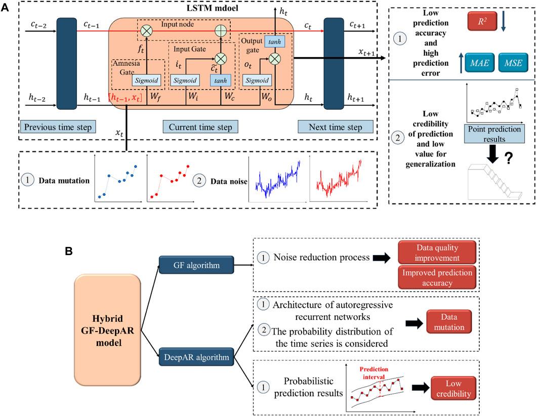
Figure 2. Problems with the LSTM model and advantages of the GF-DeepAR model (A) Problems with the LSTM model; (B) Advantages of the GF-DeepAR model.

The GF-DeepAR hybrid model-building process is shown in Figure 3. It mainly includes three parts: filtering and noise reduction processing based on the GF algorithm, slope deformation prediction based on DeepAR, and point prediction performance evaluation and comparative analysis.

Figure 3

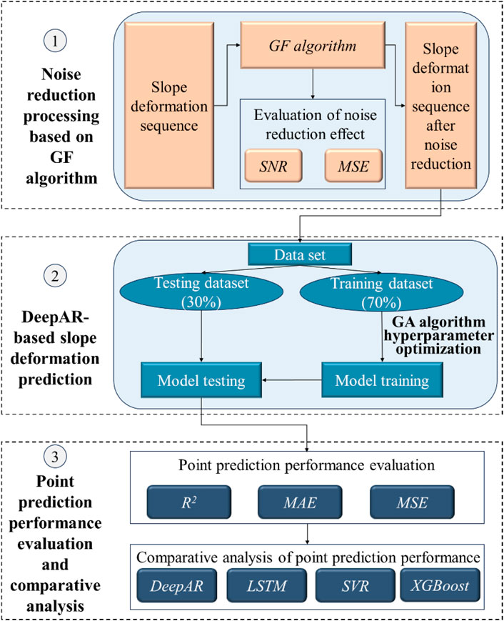
Figure 3. GF-DeepAR hybrid model.

2.3.1 Filtering and noise reduction process based on GF algorithm

The core of the GF algorithm for noise reduction lies in determining the weight matrix of the Gaussian kernel function $w_k\left(x+i,\sigma \right)$. Firstly, the filter window length (2L+1), the number of iterations K, and the standard variance $\sigma$ of the slope deformation sequence function $f\left(x\right)$ are defined. Calculate the weight matrix centered on the sampling point with Gaussian kernel function influence radius L. Normalise the weight matrix so that the sum of the weights is equal to 1 to get the final weight matrix, multiply the weight matrix with the corresponding points of the original data and then accumulate them to calculate the filtered output value $f_{k+1}\left(x\right)$ of the slope deformation sequence function $f\left(x\right)$, as shown in Eq. 8:

$f_{k+1}\left(x\right)={\displaystyle \sum _{-L}^L}{\mathrm{f}}_k\left(x+i\right)w_k\left(x+i,\sigma \right)(8)$

Repeat the above steps until the number of iterations k=K to get the slope deformation sequence after noise reduction by the GF algorithm. The signal-to-noise ratio SNR and mean square error MSE are used as noise reduction performance evaluation metrics to select the optimal noise reduction data (Chicco et al., 2021; Kononchuk et al., 2022). Where SNR and MSE are defined, as shown in Eqs 9, 10:

$\text{SNR}=10*\lg \left[{\displaystyle \sum _{i=1}^N}{x}_i^2/{\displaystyle \sum _{i=1}^N}{\left(d_i-x_i\right)}^2\right](9)$

$\text{MSE}=\frac{1}{N}{\displaystyle \sum _{i=1}^N}{\left(d_i-x_i\right)}^2(10)$

Where: x is the initial slope deformation sequence, $d_i$ is the slope deformation sequence after noise reduction, and N is the length of the slope deformation sequence. If the corresponding SNR and MSE of the noise reduction data are larger and smaller, it indicates that the noise reduction effect is better, and the data with the optimal noise reduction effect is selected for the next processing.

2.3.2 DeepAR-based slope deformation prediction

The noise-reduced slope deformation sequences are input into the DeepAR model and the data set is constructed based on the input sequences. In the specific construction process, the sliding window method is used to construct the input features and output features for slope deformation prediction. The input features $S_1,S_2,S_3......S_{t-1}$ of the data set consist of historical slope deformation values, and the time step of historical slope deformation is set to 8 with reference to the established research (Muneeb, 2022; Liu et al., 2024). The output features $S_t$ consist of slope deformation values at time t. Further, the data set is divided on the basis of the constructed data set using the Holdout method (Mao et al., 2019), which divides the data set into training and testing sets in the ratio of 7:3 according to the chronological order.

The training set is input into the model to perform the training of the prediction model. It is worth noting that the DeepAR model has many hyperparameters, such as the number of network layers (num_layers), the number of cells (num_cells), the dropout rate (dropout_rate), the learning rate (learning_rate), and the number of training rounds (epochs). In this paper for more efficient implementation of hyperparameter setting, genetic algorithm (GA) (Cai et al., 2020) is introduced for hyperparameter optimization. After completing the DeepAR model training, the optimal hyperparameters and test set are sent to the model to perform test predictions of the model. In addition, the computing environment is configured in Windows 11 using python 3.10, Core i9-14900KF, RTX4090D, 64 GB DDR5. Computational libraries such as tensorflow, pandas, etc. are used during the computation.

2.3.3 Evaluation and comparative analysis of point prediction performance

The goodness of fit (R²), mean absolute error (MAE), and mean absolute percentage error (MAPE) are selected to assess the point prediction performance of the model, which are defined as shown in Eqs 11–13:

$R^2=1-\frac{{\displaystyle \sum _{i=1}^N}{\left(y_t-{\hat{y}}_t\right)}^2}{{\displaystyle \sum _{i=1}^N}{\left(y_t-\overline{y}\right)}^2}(11)$

$MAE=\frac{1}{N}{\displaystyle \sum _{t=1}^N}\left|y_t-{\hat{y}}_t\right|(12)$

$MAPE=\frac{100\%}{N}{\displaystyle \sum _{t=1}^N}\left|\frac{y_t-{\hat{y}}_t}{y_t}\right|(13)$

Where: the larger the value of R², the higher accuracy of the prediction model. MAE and MAPE are the error metrics, the smaller its value, the smaller the prediction error. N is the number of predicted samples, $y_t$ is the measured slope deformation value, ${\hat{y}}_t$ is the predicted slope deformation value, and $\overline{y}$ is the average of the measured slope deformation value.

To further validate the prediction performance of the DeepAR model, the prediction performance of three typical prediction algorithms, LSTM, XGBoost (Asselman et al., 2023), and SVR, was compared based on the above three metrics.

3 Case studies

3.1 Case 1

3.1.1 Overview of works

To verify the effectiveness of the proposed hybrid GF-DeepAR slope deformation prediction model, a cut slope is selected as an example of a work point. As shown in Figure 4A, the slope is a secondary slope with an overall height of 8–10 m, with a wide platform of about 1.5 m in the middle. The slope is composed of vegetative fill, pebble soil, and gravel soil in order from top to bottom. The slope is protected by a slurry masonry schist retaining wall, but under the influence of the external environment, there are localized outgrowths and damages of the schist on the slope surface, which seriously affects the overall stability of the slope and the retaining wall. Therefore, two surface deformation gauges of model JMYC-623000AD, C1 and C2, are deployed at the top of the primary and secondary slopes, to monitor the deformation values of the slopes. The monitoring cycle is 200d in total, the monitoring frequency is 4h/time, the monitoring frequency can be appropriately strengthen according to the development of slope deformation, and the daily monitoring value is taken as the average of all the monitoring values of the day. The technical parameters of the surface deformation gauges and their specific placement can be found in Figure 4B.

Figure 4

Figure 4. Slope engineering and deformation measurement point layout map-Case 1 (A) Actual site view; (B) Placement of deformation measurement points.

The change rule of C1 and C2 measurement points is plotted as shown in Figure 5. The deformation of the secondary slope (measurement point C2) is larger than that of the primary slope (measurement point C1) in the figure, and this rule agrees with the established studies (Liu et al., 2024; Ye et al., 2024). Among them, the deformation of the C2 measurement point is gradually stabilized with the accumulation of time, but the fluctuation of the value before 100 days is larger, which is mainly considered to be caused by the freezing and expansion due to the environmental conditions of the site. Since then, the deformation of the C2 measurement point has gradually leveled off, but there is also a small fluctuation phenomenon, mainly considering the effect of noise (Ali et al., 2020; Duan et al., 2024). Similar to the C2 measurement point, the deformation of the C1 measurement point also tends to stabilize with time, and the cumulative deformation of the whole process is within 15 mm, but there are fluctuations in the value of the change process.

Figure 5

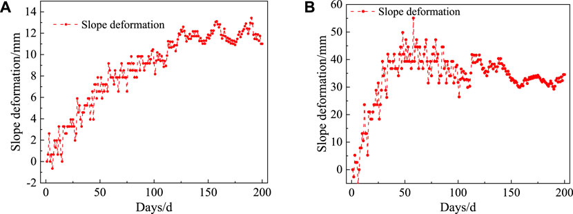
Figure 5. Change rule of slope cumulative deformation-Case 1 (A) C1 measurement point; (B) C2 measurement point.

3.1.2 Results of noise reduction analysis

The GF-DeepAR hybrid model is used to firstly reduce the noise of the original monitoring data sets Data_set_C1 and Data_set_C2 of C1 and C2 measurement points respectively (the standard deviation $\sigma$ is set to be divided into 2.0, 1.0, and 0.5), and then the relationship between the noise-reduced slope deformation series and the original noise-containing slope deformation series is shown in Figure 6.

Figure 6

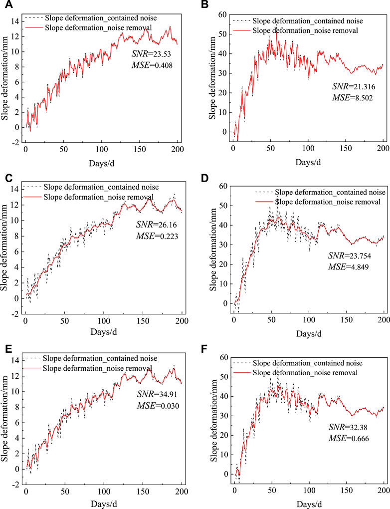
Figure 6. Noise reduction results of GF algorithm for slope deformation-Case 1 (A) C1 measurement point -σ2.0; (B) C2 measurement point -σ2.0; (C) C1 measurement point -σ1.0; (D) C2 measurement point -σ1.0; (E) C1 measurement point -σ0.5; (F) C2 measurement point -σ0.5.

As shown in Figure 6, the noise-reducing deformation series retains the characteristics of the deformation trend of the original series, and at the same time, the noise-reducing deformation series has a better smoothness than the original series, and the noise-reducing effect is better. At the C1 measurement point, SNR and MSE are 23.53(0.408), 26.16(0.223), and 34.91 (0.030) for the three different standardized variances, respectively. As the standard variance σ decreases, SNR gradually increases from 23.53 to 34.91, and MSE gradually decreases from 0.408 to 0.030, indicating that the noise reduction effect gradually becomes better, considering that the noise reduction effect obtained by continuing to reduce the standard variance σ is gradually stable, the noise reduction data under the condition that the standard variance σ is 0.5 can be selected as the data for the subsequent prediction and analysis of the C1 measurement points. At the C2 measurement point, SNR and MSE are 21.316(8.502), 23.754(4.849), and 32.38 (0.666) for the three different standardized variances, respectively. As the standard variance σ decreases, SNR gradually increases from 21.316 to 32.38, and SNR gradually decreases from 8.502 to 0.666, indicating that the effect of noise reduction gradually becomes better. Hence, the noise reduction data under the condition of standard variance σ of 0.5 is selected as the data for the subsequent prediction and analysis.

In summary, the data preprocessing part of the GF-DeepAR hybrid model can pre-filter the original monitoring data set, which retains the characteristics of the deformation trend containing the original series. At the same time, it can better eliminate the noise information hidden in it, which ensures the quality of the data for the subsequent deformation prediction and analysis of slope engineering.

3.1.3 Results of slope deformation prediction

The optimization results of the GA algorithm on the C1 and C2 measurement points are shown in Figure 7. The analysis shows that the fitness value (MAE) decays rapidly as the number of optimizations increases and stabilizes after 25 generations, indicating that the prediction error of the DeepAR model can be reduced by the GA algorithm. At the end of the optimization, the optimal hyperparameters on the C1 measurement point are obtained as num_layers=2, num_cells=120, dropout_rate=0.2, learning_rate=0.00136, and epochs=500, and the optimal hyperparameters on the C2 measurement point are obtained as num_layers=3, num_cells=200, dropout_rate=0.2, learning_rate=0.0008, epochs=500.

Figure 7

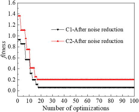
Figure 7. Optimization results of GA algorithm on C1 and C2 measurement points.

After obtaining the optimal hyperparameters, they are input into the DeepAR model. The $D_{test\_C1}$ and $D_{test\_C2}$ of C1 and C2 measurement points after the noise reduction process are input into the trained DeepAR prediction model respectively, and the corresponding slope deformation prediction results are calculated. To visualize the prediction ability of the GF-DeepAR model, the predicted results of the model at the C1 and C2 measurement points are plotted as shown in Figures 8A, B, with the horizontal axis representing the slope deformation obtained from the actual monitoring, and the vertical axis representing the slope deformation obtained from the prediction. Generally, a larger $R^2$ indicates a better nonlinear mapping ability of the model, and the noise-reduced values of C1 and C2 measurement points are 0.956 and 0.929, respectively, which are greater than 0.9, indicating a high prediction accuracy. Meanwhile, at the C1 and C2 measurement points, most of the data points are around the 45° median axis, indicating that the GF-DeepAR model has a strong ability to fit the nonlinearities against the slope deformation.

Figure 8

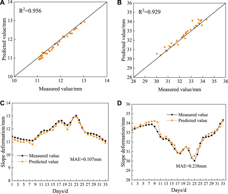
Figure 8. GF-DeepAR model slope deformation prediction results-Case 1 (A) C1 Measurement point- Scatter comparison of measured and predicted values; (B) C2 Measurement point- Scatter comparison of measured and predicted values; (C) C1 Measurement point- Comparison of measured and projected value trends; (D) C2 Measurement point- Comparison of measured and projected value trends.

Further, the comparison of the predicted and measured values of slope deformation at the C1 and C2 measurement points are shown in Figures 8C, D. The analysis shows that the GF-DeepAR prediction model can well reflect the upward and downward fluctuations of slope deformation, and the predicted values match the overall trend of the measured values with high correlation. Meanwhile, the residuals at the C1 and C2 measurement points are overall controlled within a small range, with a small mean absolute error MAE of 0.107 and 0.238, respectively.

In summary, the GF-DeepAR prediction model effectively solves the problem of accuracy improvement caused by poor data quality in slope engineering. The GF-DeepAR model shows high generalization ability on the two slope deformation measurement points, high overall prediction accuracy and small prediction error, which can well support the prediction of slope deformation.

3.1.4 Comparative analysis of slope deformation prediction before and after noise reduction

The results of the slope deformation prediction accuracy assessment before and after noise reduction at the C1 and C2 measurement points are shown in Figures 9A, B. The R², MAE, and MAPE obtained from the C1 measurement point before noise reduction are 0.875, 0.186, and 1.552%, respectively, and the R², MAE, and MAPE obtained after noise reduction are 0.956, 0.107, and 0.913%, respectively, with an increase of 0.081 in R², which indicates that the prediction accuracy of the C1 measurement point has been improved after the noise reduction treatment, while the MAE and MAPE have decreased by 0.079% and 0.639%, respectively. indicating that the prediction error of the C1 measurement point was controlled after noise reduction treatment. Similarly, after the noise reduction treatment, the C2 measurement point R² increased by 0.089, while MAE and MAPE decreased by 0.184% and 0.581%, respectively, indicating that the prediction accuracy and prediction error of the C2 measurement point were also improved after the noise reduction treatment.

Figure 9

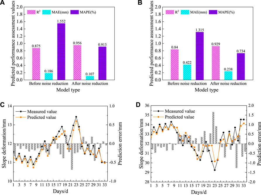
Figure 9. Comparison of slope deformation prediction results before and after noise reduction- Case 1 (A) C1 Measurement points - accuracy assessment of slope deformation prediction results before and after noise reduction; (B) C2 Measurement points - accuracy assessment of slope deformation prediction results before and after noise reduction; (C) C1 Measurement points - before and after noise reduction; (D) C2 Measurement points - before and after noise reduction.

This is mainly due to three advantages of combining GF algorithms with machine learning algorithms. Firstly, the noise in the slope deformation data can be removed by GF algorithm, making the slope deformation closer to the real situation (Innes et al., 2021; Richardson et al., 2022). Secondly, the GF algorithm not only reduces noise but also helps to highlight the intrinsic characteristics of the data (Noguer et al., 2022; Guan et al., 2024). During the filtering process, the algorithm is able to retain the main trends in the data while weakening random fluctuations. This makes it easier for machine learning algorithms to capture key information about the data during subsequent predictions, thereby improving prediction accuracy (Demšar and Zupan, 2021; Peng and Lee, 2021). Finally, with the GF algorithm, the risk of overfitting of machine learning predictive models can be reduced, and the generalization ability of the model can be improved so that it can maintain a high prediction accuracy in the face of new data.

The comparison between the predicted and measured values of slope deformation at C1 and C2 measurement points before noise reduction is shown in Figures 9C, D. The analysis shows that although the prediction results and the measured values are more closely matched as a whole, there are fluctuations at more positions, i.e., the residuals of the data are larger, while the prediction results after noise reduction have a very high correlation between the predicted values and the measured values as a whole, and the prediction effect is better. In addition, the C1 and C2 measurement points experienced relatively large mutation phenomena in the interval segment from the 17th day to the 25th day, which is mainly considered to be the influence of the monitoring equipment, external environment (Yu et al., 2021; Yang et al., 2023). The GF-DeepAR prediction model can well control the unfavorable effects of the mutation data, and the prediction results still fit closely with the measured results. On the contrary, the single DeepAR prediction model without a noise reduction process has a large prediction error in this interval, limiting the overall prediction accuracy.

In summary, the GF-DeepAR prediction model can perform noise reduction for the original dataset, which guarantees the quality of the input dataset, and the resulting prediction accuracy is higher than that of the single DeepAR prediction model, and the prediction error is lower than that of the single DeepAR prediction model.

3.1.5 Comparative analysis of the results of slope deformation prediction

To verify the superiority of the DeepAR model over the classical LSTM, XGBoost, and SVR prediction models, the same GF algorithm is used to optimize the LSTM, XGBoost, and SVR. A comparison analysis is performed with the GF-DeepAR hybrid model, and the results are shown in Figure 10. Taking the C1 measurement point as an example, the model with the smallest prediction error MAE and MAPE is the GF-DeepAR model, with MAE and MAPE of 0.107% and 0.913%, respectively, followed by the GF-LSTM model (0.151, 1.287%), then the GF-XGBoost model (0.164, 1.413%), and finally the GF-SVR model (0.891, 1.601%). Meanwhile, the prediction accuracy metric R² of each model is compared and it is found that the highest prediction accuracy is also achieved by the GF-DeepAR model. Hence, it can be obtained that the GF-DeepAR model has a better advantage in slope deformation point prediction than the classical LSTM, XGBoost and SVR models.

Figure 10

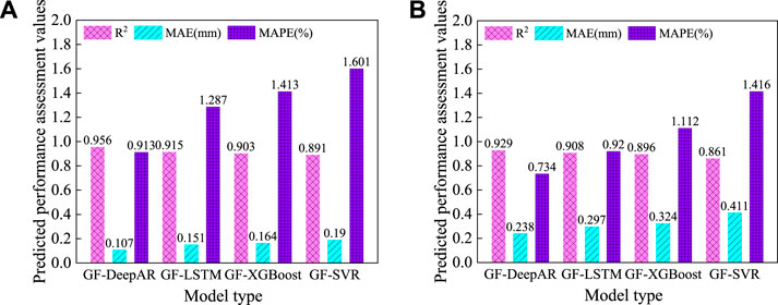
Figure 10. Comparison of prediction performance between different point prediction models (A) C1 measurement point; (B) C2 measurement point.

3.2 Case 2

3.2.1 Overview of works

Similarly, to verify the effectiveness of the proposed hybrid GF-DeepAR model, a high slope in a mountainous area is selected as an engineering example as shown in Figures 11A, B. The slope is a naturally high steep slope, the steepest part of the slope is as high as 76 m, according to the engineering geological conditions and the height of the slope to adopt step-type slope, the slope rate is set at 1:0.75 and 1:0.5. After operating for some time, there are large cracks appeared on the slope steps, and the whole slope is extruded and deformed at the foot of the slope after lateral shift, with poor slope stability. The slope is relatively high and steep, with a high-risk factor, and the consequences would be very serious in case of a landslide. To ensure the normal operation of the line, deformation monitoring is carried out for this slope.

Figure 11

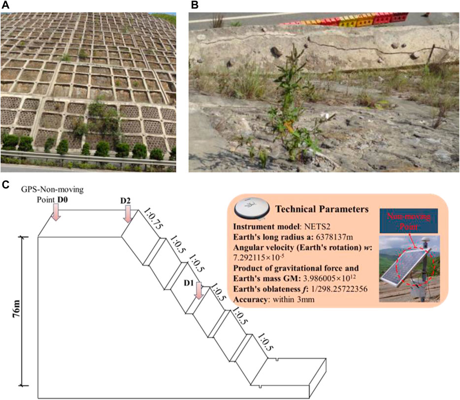
Figure 11. Slope engineering and deformation measurement point layout - Case 2 (A) High Steep Slope Site View; (B) Slope step cracks; (C) Deformation measurement point layout.

Two GPS points, D1 and D2, are placed at the middle and top of the high slope to monitor the deformation value of the slope, where the GPS receiver is modeled as NETS2. The monitoring cycle is 195 d. The monitoring frequency is set to 6 h/time, influenced by the solution cycle, and the daily monitoring values are averaged over all the monitoring values for the day. The technical parameters of the surface deformation gauges and their specific placement can be found in Figure 11C.

The change rule of D1 and D2 measurement points is plotted as shown in Figure 12. In the figure, the deformation at the top of the slope (measurement point D2) is larger than the deformation in the middle of the slope (measurement point D1), and this pattern is consistent with measurement points C1 and C2. The deformations at both D1 and D2 measurement points are cumulative over time, and there are certain fluctuations, so D1 and D2 measurement points can be used as typical measurement points to verify whether the proposed GF-DeepAR model can accurately and reliably predict the development trend of cumulative deformation of slopes.

Figure 12

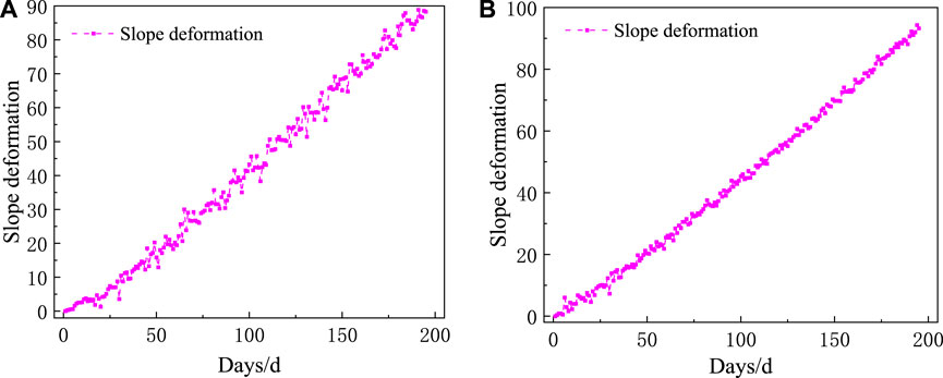
Figure 12. Change rule of slope cumulative deformation-Case 2 (A) D1 measurement point; (B) D2 measurement point.

3.2.2 Results of noise reduction analysis

The GF-DeepAR hybrid model is used to first reduce the noise of the original monitoring data sets Data_set_D1 and Data_set_D2 at D1 and D2 respectively (the standard deviation σ is set to 2.0, 1.0, and 0.5), and the relationship between the noise-reduced slope deformation series and the original noise-containing slope deformation series is shown in Figure 13.

Figure 13

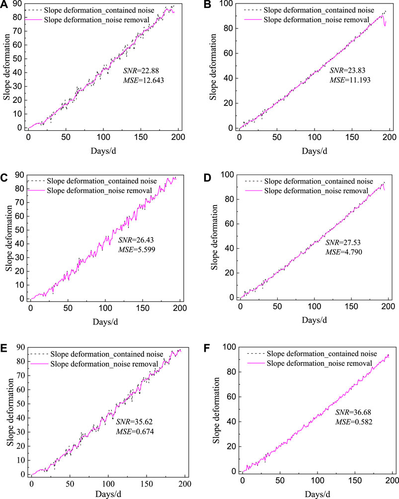
Figure 13. Noise reduction results of GF algorithm for slope deformation - Case 2 (A) D1 Measurement points -σ2.0; (B) D2 Measurement points -σ2.0; (C) D1 Measurement points -σ1.0; (D) D2 Measurement points -σ1.0; (E) D1 Measurement points -σ0.5; (F) D2 Measurement points -σ0.5.

As shown in Figure 13, the noise-reduced slope deformation series retains the characteristics of the changing trend of the original series while better removing the noise information hidden in it as in Case 1. Taking the D1 measurement point as an example, under three different standard variances, SNR and MSE are 22.88(12.643), 26.43(5.599), and 35.62 (0.674) for the three different standardized variances, respectively. SNR gradually increases from 22.88 to 35.62, and MSE gradually decreases from 12.643 to 0.674 as the standard variance $\sigma$ decreases, which indicates that the effect of noise reduction becomes better. Similarly, the results of the noise reduction performance of D2 and D1 are consistent. Considering that the noise reduction effect obtained by continuing to reduce the standard variance σ is gradually stable, the noise reduction data under the condition that the standard variance σ is 0.5 can be selected as the data for the subsequent prediction analysis of the D1 measurement point and D2.

3.2.3 Results of slope deformation prediction

Similarly, the optimization results of GA algorithm on D1 and D2 monitoring points are obtained as shown in Figure 14. Similar to the results for the C1 and C2 measurement points, the fitness value (MAE) decays rapidly as the number of optimizations increases and stabilizes after 25 generations. At the end of the optimization, the optimal hyperparameters on the D1 measurement point are obtained as num_layers=3, num_cells=67, dropout_rate=0.2, learning_rate=0.00230, and epochs=300, and the optimal hyperparameters on the D2 measurement point are obtained as num_layers=2, num_ cells=156, dropout_rate=0.2, learning_rate=0.0050, epochs=600.

Figure 14

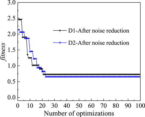
Figure 14. Optimization results of GA algorithm on D1 and D2 measurement points.

Similarly, the sequences of D1 and D2 measurement points after the noise reduction process are input into the trained DeepAR prediction model respectively, and the corresponding slope deformation prediction results are calculated and plotted as shown in Figure 15A, B. The R² after noise reduction at the D1 and D2 measurement points are 0.968 and 0.974, respectively, which are greater than 0.95, indicating a high prediction accuracy. Further, the comparison of the predicted and measured values of slope deformation at the D1 and D2 measurement points are shown in Figures 15C, D. The analysis shows tat the GF-DeepAR prediction model can well reflect the upward and downward fluctuations of slope deformation, and the predicted values match the overall trend of the measured values with high correlation. Meanwhile, the residuals at the D1 and D2 measurement points are overall controlled within a small range, with a small mean absolute error MAE of 0.811 and 0.760, respectively.

Figure 15

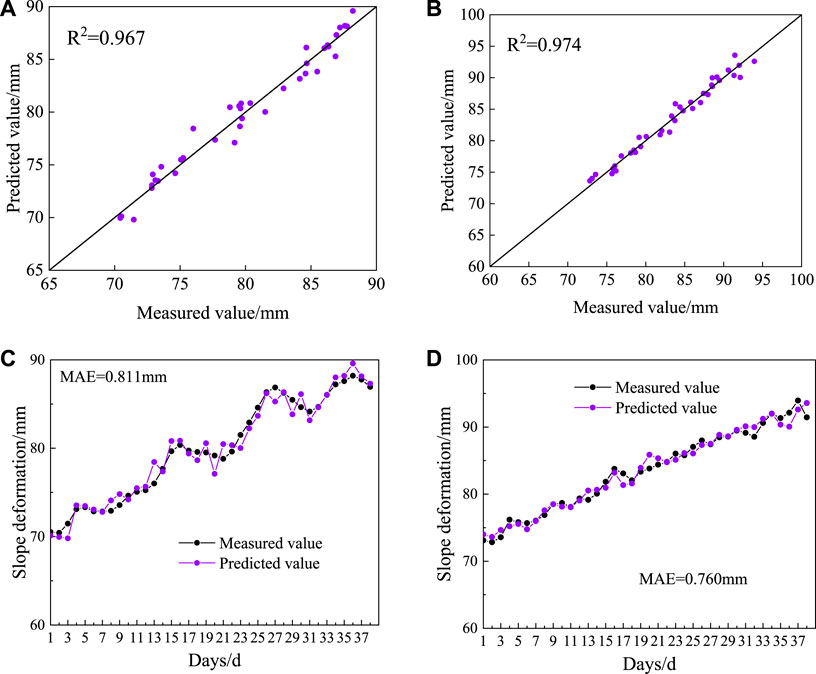
Figure 15. GF-DeepAR model slope deformation prediction results - Case 2 (A) D1 Measurement Points - Scatter Comparison of Measured and Predicted Values; (B) D2 Measurement Points - Scatter Comparison of Measured and Predicted Values; (C) D1 Measured points - comparison of measured and predicted trends; (D) D2 Measured points - comparison of measured and predicted trends.

In summary, the GF-DeepAR prediction model also effectively solves the problem of accuracy improvement due to data quality issues and the shortcomings of overfitting or underfitting of the prediction model in the high slope project in this mountainous area.

3.2.4 Comparative analysis of slope deformation prediction before and after noise reduction

The results of slope deformation prediction accuracy assessment before and after noise reduction at D1 and D2 measurement points are shown in Figure 16A, B. Taking the D1 measurement point as an example, the R², MAE and MAPE obtained before noise reduction are 0.897, 1.548, and 1.929%, respectively, and the R², MAE and MAPE obtained after noise reduction are 0.967, 0.811, and 1.017%. The increase of R² by 0.070 indicates that the prediction accuracy of the D1 measurement point is improved after the noise reduction treatment, whereas the decrease of MAE and MAPE by 0.737% and 0.912%, respectively, indicates that the prediction error of the D1 measurement point is controlled after the noise reduction treatment. The same as Case 1, the prediction accuracy of GF-DeepAR model can be effectively improved because of the three advantages of reducing noise interference, highlighting data features and improving model generalization ability.

Figure 16

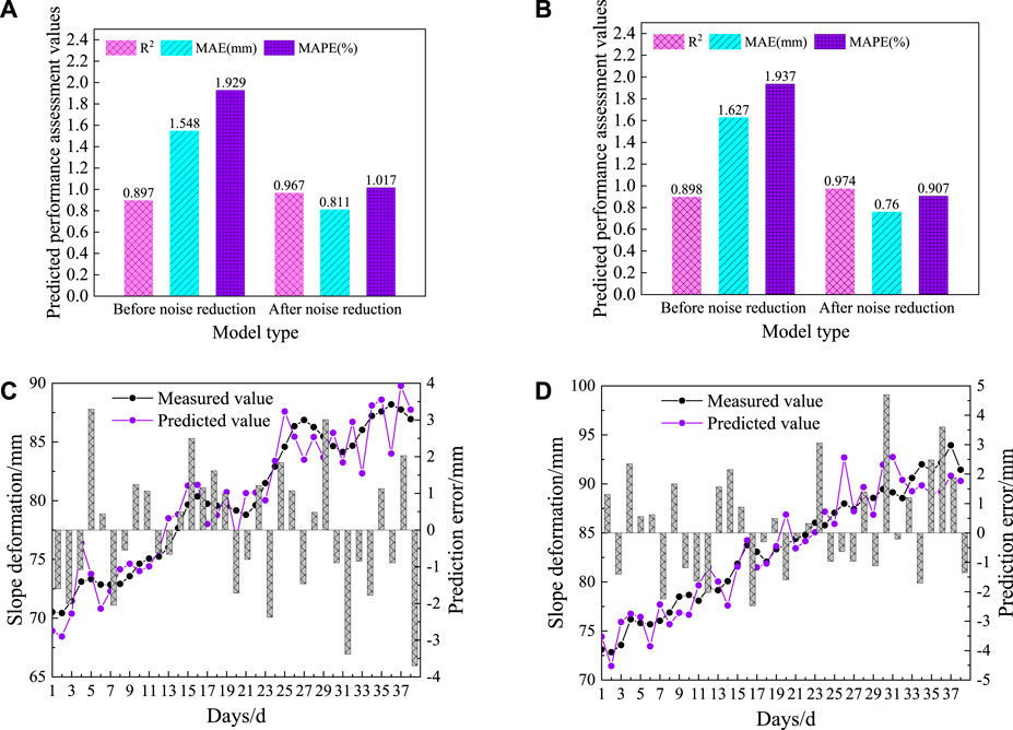
Figure 16. Comparison of slope deformation prediction results before and after noise reduction-Case 2 (A) D1 Measurement points - accuracy assessment of slope deformation prediction results before and after noise reduction; (B) D2 Measurement points - accuracy assessment of slope deformation prediction results before and after noise reduction; (C) D1 Measurement points - before and after noise reduction; (D) D2 Measurement points - before and after noise reduction.

A comparison of the predicted and measured values of slope deformation at the D1 and D2 measurement points before noise reduction is shown in Figure 16C, D. Taking the D1 measurement point as an example, the analysis shows that the fluctuation between the prediction result and the measured value exists at more positions, and the R² is lower than 0.9, which mainly considers the influence of the data noise and restricts the fit between the prediction result and the measured value; while the overall correlation between the predicted value and the measured value after the noise reduction is extremely high, and the prediction result is better. In addition, D1 and D2 measurement points experienced relatively large mutations in the interval segment from the 16th day to the 27th day. As with the results obtained in Case 1, the GF-DeepAR prediction model can well control the unfavorable effects of the mutation data, while the single DeepAR prediction model without a noise reduction process has a large prediction error in this interval.

3.2.5 Comparative analysis of the results of slope deformation prediction

Similarly, to verify the superiority of the DeepAR model over the classical LSTM, XGBoost, and SVR models, the performance assessment results of each model are calculated as shown in Figure 17. Taking the D1 measurement point as an example, the model with the smallest prediction error MAE and MAPE is the GF-DeepAR model, with MAE and MAPE of 0.811% and 1.017%, followed by the GF-LSTM model (0.951, 1.197%), then the GF-XGBoost model (1.234, 1.501%), and finally the GF-SVR model (1.340, 1.723%). Similarly, the prediction accuracy metric R² of each model is compared and it is found that the highest prediction accuracy is also achieved by the GF-DeepAR model. Hence, it can be obtained that the GF-DeepAR model has a better advantage over the classical LSTM, XGBoost, and SVR models in the prediction of slope deformation points.

Figure 17

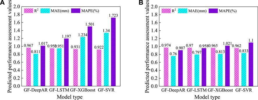
Figure 17. Comparison of prediction performance between different point prediction models (A) D1 measurement point; (B) D2 measurement point.

4 Framework for probability analysis of slope deformation based on the GF-DeepAR model

Compared with GF-LSTM, GF-XGBoost, and GF-SVR models, the GF-DeepAR model has better prediction performance. Moreover, the GF-DeepAR model can take into account the uncertainty of slope deformation prediction and provide the probability distribution of the slope deformation prediction results, which is more conducive to making safety precautionary decisions (Deng et al., 2023).

The probability analysis framework of the GF-DeepAR model is shown in Figure 18. In this paper, we use historically measured slope deformation data to predict the slope deformation sequence probabilistically based on the GF-DeepAR model, and assess the prediction performance by using three metrics, namely, the prediction interval coverage (PICP), the normalized average width of the prediction interval (PINAW), and the coverage width criterion (CWC) (Shi et al., 2022; Schmidinger and Heuvelink, 2023). The specific calculations are as shown in Eqs 14–18:

$PICP=\frac{1}{N}{\displaystyle \sum _{k=1}^N}{R}_k(14)$

$R_k=\left\{\begin{array}{l}1,Y\left(k\right)\in \left[Y_{low},Y_{high}\right]\\ 0,Y\left(k\right)\notin \left[Y_{low},Y_{high}\right]\end{array}\right.(15)$

$PINAW=\frac{1}{N\left(Y_{\max }-Y_{\min }\right)}{\displaystyle \sum _{k=1}^N}\left(Y_{high}-Y_{low}\right)(16)$

$CWC=PINAW\left[1+I\left(PICP\right)e^{-p\left(PICP-\nu \right)}\right](17)$

$I\left(PICP\right)=\left\{\begin{array}{l}1,PICP<\nu \\ 0,Others\end{array}\right.(18)$

Figure 18

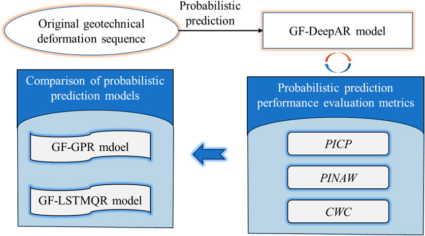
Figure 18. Framework for probabilistic analysis of the GF-DeepAR model.

Where: $Y_{high}$, $Y_{low}$ are the maximum and minimum values of a sample prediction interval in the slope deformation sequence $Y_{\max }$, $Y_{\min }$ are the maximum and minimum values of all predicted samples. $\nu$ is set as the nominal confidence level, $p$ is the penalty parameter for the probability of failure intervals, which ranges from 50 to 100, and is taken as 50 here. A larger PICP indicates that there are more true values in the prediction interval, and a smaller PINAW has a smaller range of the prediction interval, which is more favorable for decision making. PICP and PINAW can be combined through CWC, and the smaller the value of CWC, the better.

The probability prediction analysis is carried out on the C1 and the D1 measurement point in Case 1 and Case 2, based on the GF-DeepAR model. The probability prediction results under the condition of 95% confidence are obtained as shown in Figure 19. The prediction intervals constructed in Figure 19, indicate that the PICP in both C1 and D1 measurement points are 100%, which is far from meeting the requirement of a 95% confidence level, implying that the prediction intervals constructed by the GF-DeepAR model can effectively envelope the actual slope deformation curves, and the PINAW are low, which are 0.330% and 0.256% respectively. It indicates that the upper and lower boundaries of the interval can be used as optimistic and conservative estimation quantities for slope deformation prediction. Taking the C1 measurement point shown in Figure 19A as an example, when the boundary value of the interval is lower than the corresponding engineering deformation warning index, it means that the actual deformation has a corresponding probability of being in the safe range. Hence, the probabilistic prediction provides an effective method for quantitatively evaluating the safety risk of slopes.

Figure 19

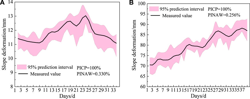
Figure 19. Probabilistic prediction results for C1 and D1 measurement points (A) C1 probability prediction results; (B) D1 probability prediction results.

As shown in Figure 18, to verify the superiority of GF-DeepAR model in probability prediction, GF-GPR and GF-LSTMQR models are used for the comparation analysis of slope deformation probability prediction. The results of the comparison of prediction performance between different probability prediction models are obtained as shown in Figure 20. The PICP of the GF-DeepAR and GF-GPR models can reach 100% at both C1 and D1 measurement points, followed by the GF-LSTMQR model (C1: 96.97%, D1: 94.73%). Meanwhile, it can be found that the width of the GF-LSTMQR model is much larger than that of the remaining two types of models by PINAW values, which suggests that the GF-LSTMQR model has a larger degree of uncertainty. From the comparison analysis of the reliability and uncertainty of the intervals, the CWC values of the GF-DeepAR model proposed in this paper are 0.330% and 0.256% in the two measurement points of C1 and D1, respectively. They are smaller than the rest of the two types of models, indicating that the method in this paper not only meets the requirement of the reliability of the confidence level but also constructs intervals with the smallest uncertainty.

Figure 20

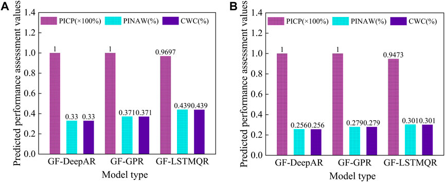
Figure 20. Comparison of prediction performance between different probabilistic prediction models (A) C1 measurement point; (B) D1 measurement point.

In summary, it indicates that the GF-DeepAR model is superior in probability prediction and better compared to the GF-GPR and GF-LSTMQR models. In addition, the GF-DeepAR probability prediction model also provides managers with an effective tool to quantify the uncertainty of the model output results, which can be used to analyze the main factors that cause uncertainty in the results on time according to the probability of interval coverage and the width of the intervals, to carry out timely regulation and reduce the risk of decision-making.

5 Discussions

In order to better highlight the research innovation of this paper, it is discussed and analyzed in three parts: comparison with similar studies, the processing of the input data comparison of prediction accuracy at different time steps and future outlook.

5.1 Comparison with similar studies

As shown in Table 1, a comparison of the established studies and the study in this paper is organized. The established studies include ACO-SVM model, SVM model, WD-IPSO-LSTM model, Transformer model and BiLSTM model, and in this paper, we study the GF-DeepAR model. By organizing the point prediction assessment results of each model, it is found that the R², MAE, and MAPE of the GF-DeepAR model are optimal, indicating that the GF-DeepAR model can achieve better prediction accuracy and lower prediction error. Meanwhile, another advantage of the GF-DeepAR model over established studies is the probability prediction, and the GF-DeepAR model can provide highly reliable and clear probability prediction results with a PICP of 100%.

Table 1

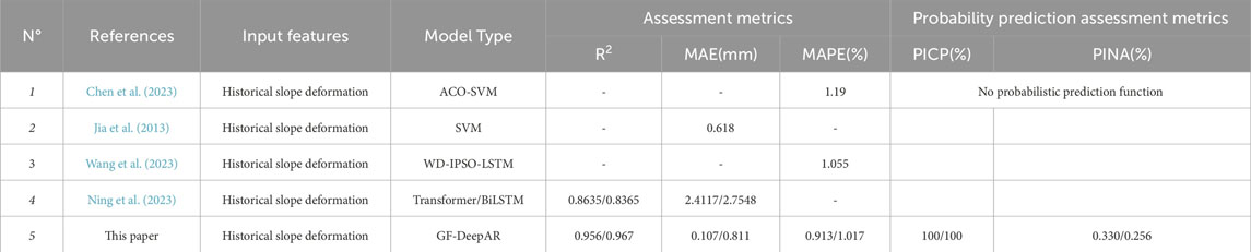
Table 1. Accuracy assessment of slope deformation prediction results before and after noise reduction-Case 2.

5.2 The processing of the input data comparison of prediction accuracy at different time steps

In order to analysis the prediction performance of the GF-DeepAR model with different input parameters, the R² of the prediction results is calculated from the setup of different slope deformation time steps (3–13). Obtained different slope deformation time step under the R² change rule as shown in Figure 21, the analysis shows that when the time step between 3 and 8, R² fluctuates up and down, and reached the best when the time step is 8. Then, as the time step increases, R² gradually decreases, mainly considering that the longer and farther away from the predicted target time the slope deformation has less influence on the predicted target (Liu et al., 2020).

Figure 21

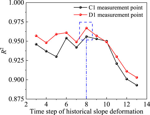
Figure 21. Different slope deformation time step under the R² change rule.

5.3 Future outlook

In this paper, a slope deformation prediction method based on the GF-DeepAR hybrid model is proposed, which can be used for noise reduction of slope noise data and provide highly accurate and reliable prediction results. However, the monitoring data of the underlying project only includes slope deformation data and the core point of this paper focuses on the noise reduction algorithm and prediction analysis, the input features of the GF-DeepAR hybrid model are only slope deformation, and the influencing factors of slope deformation are not considered. In general, water has a great influence on soft rock slopes, loose accumulation slopes, and landslide slopes, etc. (Zhang et al., 2022; Yu et al., 2023). In addition, the deformation of slopes is susceptible to rainfall, water level, water content, and other factors related to water, which can lead to sudden changes or anomalies in deformation (Lo et al., 2023), which in turn affects the performance of slope deformation prediction models. It is worth noting that rainfall characteristics may contain multiple metrics such as rainfall intensity, rainfall on the same day, rainfall over multiple days, etc., and water level characteristics may also contain multiple metrics such as the amount of change in water level and the cumulative amount of water level. To represent the influence of the main control features of slope deformation more accurately, it is necessary to screen for numerous influencing factors (Mali et al., 2021; Zhuang et al., 2023) Hence, the sensitivity analysis method can be introduced based on the existing methods to optimize the best input features for slope deformation prediction, and then carry out the subsequent point prediction and probability prediction analysis, as shown in Figure 22.

Figure 22

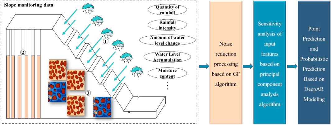
Figure 22. Future outlook.

6 Conclusion

It is important for early warning of slope instability risk to understand future patterns of slope deformation. Currently, the susceptibility of slope monitoring data to noise problems limits the accuracy and reliability of slope deformation prediction. In this paper, a slope deformation point prediction and probability analysis model based on the GF-DeepAR algorithm is proposed and validated relying on two real slope engineering cases. Some conclusions are as follows:

1) The best noise reduction is achieved at the C1 and D2 sites with a standard deviation σ of 0.5. The corresponding SNR and MSE values are 34.91 (0.030) and 35.62 (0.674).

2) A comparison before and after noise reduction reveals that the R² values for the C1 and D2 measurement points increased by 0.081 and 0.070, respectively. Additionnally, the MAE decreases from 0.079 to 0.639, and the MAPE decreases from 0.737% to 0.912%, which indicates that the accuracy of point prediction and prediction error of each measurement point is improved after noise reduction treatment.

3) The prediction intervals constructed by the GF-DeepAR model can effectively envelop the actual slope deformation curves, and the PICP in both C1 and D1 are 100%, which is far enough to meet the requirement of 95% confidence level. The PINAW is low, measuring 0.330% and 0.256% for C1 and D1, respectively.

4) Whether it is point prediction or probability prediction, the GF-DeepAR model excels at extracting feature information from slope deformation sequences characterized by randomness and complexity. It conducts predictions with high accuracy and reliability, indicating superior performance compared to other models.

Data availability statement

The original contributions presented in the study are included in the article/supplementary material, further inquiries can be directed to the corresponding author.

Author contributions

MS: Conceptualization, Formal Analysis, Methodology, Software, Validation, Visualization, Writing–original draft. FL: Data curation, Funding acquisition, Investigation, Project administration, Resources, Supervision, Writing–review and editing.

Funding

The author(s) declare that financial support was received for the research, authorship, and/or publication of this article. This research was funded by the National Natural Science Foundation of China (No. 52378439).

Conflict of interest

Author MS was employed by Hunan Provincial Communications Planning, Survey and Design Institute Co., Ltd. Author FL was employed by Hunan Water Planning and Design Institute Co., Ltd.

Publisher’s note

All claims expressed in this article are solely those of the authors and do not necessarily represent those of their affiliated organizations, or those of the publisher, the editors and the reviewers. Any product that may be evaluated in this article, or claim that may be made by its manufacturer, is not guaranteed or endorsed by the publisher.

References

Ali, Y., Irfan, M., and Hussain, E. (2020). The impact of data noise on permanent deformation behaviour of asphalt concrete mixtures. Int. J. Pavement Eng. 21 (12), 1470–1481. doi:10.1080/10298436.2018.1549324

CrossRef Full Text | Google Scholar

Asselman, A., Khaldi, M., and Aammou, S. (2023). Enhancing the prediction of student performance based on the machine learning XGBoost algorithm. Environ 31 (6), 3360–3379. doi:10.1080/10494820.2021.1928235

CrossRef Full Text | Google Scholar

Cai, L., Wu, Y., Zhu, S., Tan, Z., and Yi, W. (2020). Bi-level programming enabled design of an intelligent maritime search and rescue system. Adv. Eng. Inf. 46, 101194. doi:10.1016/j.aei.2020.101194

CrossRef Full Text | Google Scholar

Cao, R., Zeng, Q., Ni, W., Duan, H., Liu, C., Lu, F., et al. (2023). Business process remaining time prediction using explainable reachability graph from gated RNNs. Appl. Intell. 53 (11), 13178–13191. doi:10.1007/s10489-022-04192-x

CrossRef Full Text | Google Scholar

Cao, S., Yang, M., Hu, J., and Chen, J. (2023). Advanced perception and control method of harmful gas during construction period of coal tunnel based on DeepAR. Front. Earth Sci. 11, 1225287. doi:10.3389/feart.2023.1225287

CrossRef Full Text | Google Scholar

Chang, X., and Jia, X. (2023). A DeepAR based hybrid probabilistic prediction model for production bottleneck of flexible shop-floor in Industry 4.0. Comput. Ind. Eng. 185, 109644. doi:10.1016/j.cie.2023.109644

CrossRef Full Text | Google Scholar

Chen, J., Wei, Y., Ma, X., and Mei, G. (2023). Machine learning approaches for slope deformation prediction based on monitored time-series displacement data: a comparative investigation. Appl. Sci. 13 (8), 4677. doi:10.3390/app13084677

CrossRef Full Text | Google Scholar

Chen, M. R., Zeng, G. Q., Lu, K. D., and Weng, J. (2019). A two-layer nonlinear combination method for short-term wind speed prediction based on ELM, ENN, and LSTM. IEEE Internet Things J. 6 (4), 6997–7010. doi:10.1109/JIOT.2019.2913176

CrossRef Full Text | Google Scholar

Chicco, D., Warrens, M., and Jurman, G. (2021). The coefficient of determination R-squared is more informative than SMAPE, MAE, MAPE, MSE and RMSE in regression analysis evaluation. PeerJ Comput. Sci. 7, e623. doi:10.7717/peerj-cs.623

PubMed Abstract | CrossRef Full Text | Google Scholar

Demšar, J., and Zupan, B. (2021). Hands-on training about overfitting. Plos Comput. Biol. 17 (3), e1008671. doi:10.1371/journal.pcbi.1008671

PubMed Abstract | CrossRef Full Text | Google Scholar

Deng, L., Li, W., and Zhang, W. (2023). Intelligent prediction of rolling bearing remaining useful life based on probabilistic DeepAR-Transformer model. Meas. Sci. Technol. 35 (1), 015107. doi:10.1088/1361-6501/acf874

CrossRef Full Text | Google Scholar

Deng, L., Smith, A., Dixon, N., and Yuan, H. (2021). Automatic classification of landslide kinematics using acoustic emission measurements and machine learning. Landslides 18, 2959–2974. doi:10.1007/s10346-021-01676-8

CrossRef Full Text | Google Scholar

Dong, J., Liao, J., Huan, X., and Cooper, D. (2023). Expert elicitation and data noise learning for material flow analysis using Bayesian inference. J. Ind. Ecol. 27 (4), 1105–1122. doi:10.1111/jiec.13399

CrossRef Full Text | Google Scholar

Duan, Q., Hua, X., and Huang, Y. (2024). Noise reduction analysis of deformation data based on CEEMD-PE-SVD modeling. J. Phys. 2724, 012033. doi:10.1088/1742-6596/2724/1/012033

CrossRef Full Text | Google Scholar

Guan, S., Wang, Y., Liu, L., Gao, J., Xu, Z., and Kan, S. (2024). Ultra-short-term wind power prediction method based on FTI-VACA-XGB model. Expert. Syst. Appl. 235, 121185. doi:10.1016/j.eswa.2023.121185

CrossRef Full Text | Google Scholar

Innes, G. K., Bhondoekhan, F., Lau, B., Gross, A. L., Ng, D. K., and Abraham, A. G. (2021). The measurement error elephant in the room: challenges and solutions to measurement error in epidemiology. Epidemiol. Rev. 43 (1), 94–105. doi:10.1093/epirev/mxab011

CrossRef Full Text | Google Scholar

Jia, L., Li, Y., and Xie, Y. (2013). Slope deformation prediction based on support vector machine. J. Eng. Sci. Technol. Rev. 6 (1), 115–118. doi:10.25103/jestr.061.23

CrossRef Full Text | Google Scholar

Jiang, F., Han, X., Zhang, W., and Chen, W. (2021). Atmospheric pm2. 5 prediction using Deepar optimized by sparrow search algorithm with opposition-based and fitness-based learning. Atmosphere 12 (7), 894. doi:10.3390/atmos12070894

CrossRef Full Text | Google Scholar

Kononchuk, R., Cai, J., Ellis, F., Thevamaran, R., and Kottos, T. (2022). Exceptional-point-based accelerometers with enhanced signal-to-noise ratio. Nature 607 (7920), 697–702. doi:10.1038/s41586-022-04904-w

PubMed Abstract | CrossRef Full Text | Google Scholar

Lasantha, D., Vidanagamachchi, S., and Nallaperuma, S. (2023). Deep learning and ensemble deep learning for circRNA-RBP interaction prediction in the last decade: a review. Eng. Appl. Artif. Intell. 123, 106352. doi:10.1016/j.engappai.2023.106352

CrossRef Full Text | Google Scholar

Lin, Q., Wang, Y., Liu, T., Zhu, Y., and Sui, Q. (2017). The vulnerability of people to landslides: a case study on the relationship between the casualties and volume of landslides in China. Int. J. Environ. Res. Public Health 14, 212. doi:10.3390/ijerph14020212

PubMed Abstract | CrossRef Full Text | Google Scholar

Liu, X., Zhang, H., Kong, X., and Lee, K. Y. (2020). Wind speed forecasting using deep neural network with feature selection. Neurocomputing 397, 393–403. doi:10.1016/j.neucom.2019.08.108

CrossRef Full Text | Google Scholar

Liu, Y., Qiu, H., Kamp, U., Wang, N., Wang, J., Huang, C., et al. (2024). Higher temperature sensitivity of retrogressive thaw slump activity in the Arctic compared to the Third Pole. Sci. Total Environ. 914, 170007. doi:10.1016/j.scitotenv.2024.170007

PubMed Abstract | CrossRef Full Text | Google Scholar

Lo, C., Lai, Y., and Chu, C. H. (2023). Investigation of rainfall-induced failure processes and characteristics of wedge slopes using physical models. Water 15 (6), 1108. doi:10.3390/w15061108

CrossRef Full Text | Google Scholar

Ma, Z., Mei, G., Prezioso, E., Zhang, Z., and Xu, N. (2021). A deep learning approach using graph convolutional networks for slope deformation prediction based on time-series displacement data. Neural. comput. Appl. 33 (21), 14441–14457. doi:10.1007/s00521-021-06084-6

CrossRef Full Text | Google Scholar

Mali, N., Dutt, V., and Uday, K. V. (2021). Determining the geotechnical slope failure factors via ensemble and individual machine learning techniques: a case study in Mandi, India. Front. Earth Sci. 9, 701837. doi:10.3389/feart.2021.701837

CrossRef Full Text | Google Scholar

Mao, F., Zhou, X., and Song, Y. (2019). Environmental and human data-driven model based on machine learning for prediction of human comfort. IEEE Access 7, 132909–132922. doi:10.1109/access.2019.2940910

CrossRef Full Text | Google Scholar

Muneeb, M. (2022). LSTM input timestep optimization using simulated annealing for wind power predictions. Plos one 17 (10), e0275649. doi:10.1371/journal.pone.0275649

PubMed Abstract | CrossRef Full Text | Google Scholar

Nguyen, T. S., Yang, K. H., Wu, Y. K., Teng, F. C., Chao, W. A., and Lee, W. L. (2022). Post-failure process and kinematic behavior of two landslides: case study and material point analyses. Comput. Geotech. 148, 104797. doi:10.1016/j.compgeo.2022.104797

CrossRef Full Text | Google Scholar

Ning, X., Yang, Q., Sun, Y., and Mei, G. (2023). Machine learning approaches for slope deformation prediction based on monitored time-series displacement data: a comparative investigation. Appl. Sci. 13 (8), 4677. doi:10.3390/app13084677

CrossRef Full Text | Google Scholar

Noguer, J., Contreras, I., Mujahid, O., Beneyto, A., and Vehi, J. (2022). Generation of individualized synthetic data for augmentation of the type 1 diabetes data sets using deep learning models. Sensors 22 (13), 4944. doi:10.3390/s22134944

PubMed Abstract | CrossRef Full Text | Google Scholar

Peng, W., Song, S., Yu, C., Bao, Y., Sui, J., and Hu, Y. (2019). Forecasting landslides via three-dimensional discrete element modeling: helong landslide case study. Appl. Sci. 9, 5242. doi:10.3390/app9235242

CrossRef Full Text | Google Scholar

Peng, Y. L., and Lee, W. P. (2021). Data selection to avoid overfitting for foreign exchange intraday trading with machine learning. Appl. Soft Comput. 108, 107461. doi:10.1016/j.asoc.2021.107461

CrossRef Full Text | Google Scholar

Qiu, H., Su, L., Tang, B., Yang, D., Ullah, M., Zhu, Y., et al. (2024). The effect of location andgeometric properties of landslides caused by rainstorms andearthquakes. Earth Surf. Proc. Land., 1–13. doi:10.1002/esp.5816

CrossRef Full Text | Google Scholar

Richardson, D. B., Keil, A. P., and Cole, S. R. (2022). Amplification of bias due to exposure measurement error. Am. J. Epidemiol. 191 (1), 182–187. doi:10.1093/aje/kwab228

PubMed Abstract | CrossRef Full Text | Google Scholar

Salinas, D., Flunkert, V., Gasthaus, J., and Januschowski, T. (2020). DeepAR: probabilistic forecasting with autoregressive recurrent networks. Int. J. Forecast. 36 (3), 1181–1191. doi:10.1016/j.ijforecast.2019.07.001

CrossRef Full Text | Google Scholar

Schaduangrat, N., Anuwongcharoen, N., Charoenkwan, P., and Shoombuatong, W. (2023). DeepAR: a novel deep learning-based hybrid framework for the interpretable prediction of androgen receptor antagonists. J. Cheminformatics 15 (1), 50. doi:10.1186/s13321-023-00721-z

CrossRef Full Text | Google Scholar

Schmidinger, J., and Heuvelink, G. (2023). Validation of uncertainty predictions in digital soil mapping. Geoderma 437, 116585. doi:10.1016/j.geoderma.2023.116585

CrossRef Full Text | Google Scholar

Selva, N. S., Sindhuja, R., and Selva, K. R. (2020). Double stage Gaussian filter for better underwater image enhancement. Wireless Pers. Commun 114, 2909–2921. doi:10.1007/s11277-020-07509-6

CrossRef Full Text | Google Scholar

Shen, Y., Guo, J., Liu, X., Kong, Q., Guo, L., and Li, W. (2018). Long-term prediction of polar motion using a combined SSA and ARMA model. J. Geod. 92, 333–343. doi:10.1007/s00190-017-1065-3

CrossRef Full Text | Google Scholar

Shi, B., Yuan, Y., Zhuang, T., Xu, X., Schmidhalter, U., Ata-Ui-Karim, S., et al. (2022). Improving water status prediction of winter wheat using multi-source data with machine learning. Eur. J. Agron. 139, 126548. doi:10.1016/j.eja.2022.126548

CrossRef Full Text | Google Scholar

Singh, R., Patra, K., Pradhan, B., and Samantra, A. (2024). HDTO-DeepAR: a novel hybrid approach to forecast surface water quality indicators. J. Environ. Manage. 352, 120091. doi:10.1016/j.jenvman.2024.120091

PubMed Abstract | CrossRef Full Text | Google Scholar

Soliman, W., Zhiyuan, C., Johnson, C., and Sabrina, W. (2023). ETF markets’ prediction &amp; assets management platform using probabilistic autoregressive recurrent networks. Eurasia pro. Sci. Technol. Eng. Math. 23, 485–494. doi:10.55549/epstem.1372067

CrossRef Full Text | Google Scholar

Wang, S., Lyu, T., Luo, N., and Chang, P. (2024). Deformation prediction of rock cut slope based on long short-term memory neural network. Int. J. Mach. Learn. Cyber. 15, 795–805. doi:10.1007/s13042-023-01939-x

CrossRef Full Text | Google Scholar

Xi, N., Yang, Q., Sun, Y., and Mei, G. (2023). Machine learning approaches for slope deformation prediction based on monitored time-series displacement data: a comparative investigation. Appl. Sci. 13, 4677. doi:10.3390/app13084677

CrossRef Full Text | Google Scholar

Xie, P., Zhou, A., and Chai, B. (2019). The application of long short-term memory (LSTM) method on displacement prediction of multifactor-induced landslides. IEEE Access 7, 54305–54311. doi:10.1109/ACCESS.2019.2912419

CrossRef Full Text | Google Scholar

Xu, J., Jiang, Y., and Yang, C. (2022). Landslide displacement prediction during the sliding process using XGBoost, SVR and RNNs. Appl. Sci. 12, 6056. doi:10.3390/app12126056

CrossRef Full Text | Google Scholar

Yang, D., Qiu, H., Ye, B., Liu, Y., Zhang, J., and Zhu, Y. (2023). Distribution and recurrence of warming-induced retrogressive thaw slumps on the central qinghai-tibet plateau. J. Geophys. Res-earth. 128, e2022JF007047. doi:10.1029/2022JF007047

CrossRef Full Text | Google Scholar

Ye, B., Qiu, H., Tang, B., Liu, Y., Liu, Z., Jiang, X., et al. (2024). Creep deformation monitoring of landslides in a reservoir area. J. Hydrol. 632, 130905. doi:10.1016/j.jhydrol.2024.130905

CrossRef Full Text | Google Scholar

Yu, H., Tang, H., Zhou, J., Li, C., Zhang, H., and Zhu, W. (2023). An analytical model for assessing dynamic stability of bedding rock slope with soil interlayer under different rain patterns. Rock. Mech. Rock Eng., 1–20. doi:10.1007/s00603-023-03595-7

CrossRef Full Text | Google Scholar

Yu, X., Gong, B., and Tang, C. (2021). Study of the slope deformation characteristics and landslide mechanisms under alternating excavation and rainfall disturbance. Bull. Eng. Geol. Environ. 80, 7171–7191. doi:10.1007/s10064-021-02371-7

CrossRef Full Text | Google Scholar

Zhang, B., Zhang, M., Liu, H., Sun, P., Feng, L., Li, T., et al. (2022). Water flow characteristics controlled by slope morphology under different rainfall capacities and its implications for slope failure patterns. Water 14 (8), 1271. doi:10.3390/w14081271

CrossRef Full Text | Google Scholar

Zhang, L., Zhang, J., Ren, P., Ding, L., Hao, W., An, C., et al. (2023). Analysis of energy consumption prediction for office buildings based on GA-BP and BP algorithm. Case Stud. Therm. Eng. 50, 103445. doi:10.1016/j.csite.2023.103445

CrossRef Full Text | Google Scholar

Zhang, S., Jia, H., Wang, C., Wang, X., He, S., and Jiang, P. (2024). Deep-learning-based landslide early warning method for loose deposits slope coupled with groundwater and rainfall monitoring. Comput. Geotech. 165, 105924. doi:10.1016/j.compgeo.2023.105924

CrossRef Full Text | Google Scholar

Zhu, A., Zhao, Q., Yang, T., Zhou, L., and Zeng, B. (2024). Wind speed prediction and reconstruction based on improved grey wolf optimization algorithm and deep learning networks. Comput. Electr. Eng. 114, 109074. doi:10.1016/j.compeleceng.2024.109074

CrossRef Full Text | Google Scholar

Zhuang, W., Liu, Y., Zhang, R., Hou, S., and Qiang, Y. (2023). Study on deformation mechanism and parameter inversion of a reservoir bank slope during initial impoundment. Acta Geotech. 18, 4353–4374. doi:10.1007/s11440-023-01839-y

CrossRef Full Text | Google Scholar

Zuo, S., Zhao, L., Deng, D., Han, Z., Zhao, B., and Zhao, Z. (2022). Back analysis of shear strength parameters for progressive landslides: case study of the Caifengyan landslide, China. Bull. Eng. Geol. Environ. 81, 19. doi:10.1007/s10064-021-02507-9

CrossRef Full Text | Google Scholar