An efficient method for modeling and evaluating the bench terrain of open-pit mines

In order to quantitatively analyze the roughness of the bench floor during open-pit mine blasting, this study proposes a real-time measuring method for the three-dimensional terrain of the bench floor during the excavation process. Real-time monitoring is conducted at the boundary and discrete internal points of the workbench floor during electric shovel operation, utilizing real-time kinematic global navigation satellite system (RTK-GNSS) positioning technology. An improved convex hull algorithm is introduced to automatically extract the optimal boundary of discrete point clouds based on their spatial distribution characteristics. This study establishes a digital elevation model (DEM) using five interpolation algorithms for 3D terrain visualization simulation. Through cross-validation, a comparative analysis of the DEM accuracy, the simulation results of the ordinary kriging interpolation algorithm were found to be optimized. The optimized interpolation algorithm is applied to simulate the 3D terrain in the Dexing open-pit copper mine, and the relevant terrain parameters were calculated. This dataset can serve as a precise foundation for the real-time path planning of elevation blasting design and ground leveling operations.

1 Introduction

The effectiveness of blasting techniques in open-pit mining significantly influences economic outcomes and project timelines (Wei et al., 2022). For example, an unavoidable rock bank after a blast can affect the efficiency of shoveling and transportation and the location and depth of subsequent precise drilling. Mining technicians depend on their experience to survey the terrain of the bench surface after blasting and determine the reference height and smooth operation path; this leads to low operational efficiency and difficulty in providing digital support for subsequent bench blasting designs. Consequently, a rapid measurement technology for open pit bench floor terrain is here studied. In recent years, the global navigation satellite system (GNSS) has been widely used in the terrain measurement of open-pit mines for terrain mapping, mining area deformation monitoring, control measurement, and laying out drilling holes (Duan et al., 2015; Fang, 2019; Wang, 2020; Zhang et al., 2022a). A digital elevation model (DEM) for the bench floor is established here by collecting GNSS data. Digital information on the bench floor DEM is used for subsequent leveling operations and blasting design.

The measurement technology for bench terrain is mainly divided into vehicle carrying and unmanned aerial vehicle carrying methods. The latter requires data acquisition after excavation of the rocks that cover the surface of the bench by electric shovel. Due to limitations in battery life, unmanned aerial vehicles are unable to continuously conduct real-time measurements. Therefore, many research institutions have developed vehicle carrying GNSS rapid terrain survey methods. For example, Hokkaido University in Japan developed a laser range finder and GNSS to measure a 3D terrain map by autonomous vehicles (Yokota et al., 2004; Huang et al., 2017). Meng developed an airborne 3D terrain survey system based on real-time kinematic (RTK)-GNSS, verifying that the system had higher measurement accuracy when the vehicle runs at low speed (Meng et al., 2009). Li H.P. developed a GNSS rapid terrain measurement system for farmland to obtain static elevation measurement accuracy of less than 1 cm (Li et al., 2014). Fan et al. (2019) and Jing et al. (2019) adopted a terrain survey method based on the combination of a GNSS double antenna, an attitude heading reference system, and the RTK positioning algorithm with double antenna configuration; this effectively reduced measurement error by 10% compared to single antenna measurement. RTK technology can be employed to further improve GNSS positioning accuracy with reasonable environmental adaptability and stability (Wang et al., 2023).

The original positioning data obtained by airborne GNSS have the problems of voids, non-uniformity, and high degree of dispersion, which need to undergo filtering, classification, and interpolation to obtain high-precision DEM. The accuracy of DEM is directly affected by the interpolation algorithm, which makes the application of airborne GNSS in the study of terrain process difficult. Ordinary kriging (OK), radial basis function (RBF), inverse distance weighting (IDW), irregular network triangulated mesh (TIN), and natural neighbor (NN) interpolation algorithms can be used to simulate DEM and address the problems of voids (Bater and Coops, 2009; Erdogan, 2009; Guo et al., 2010; Shen et al., 2012; Chu et al., 2014; Lv et al., 2015; Montealegre et al., 2015; Montealegre et al., 2015; Viswanathan et al., 2015; Chen et al., 2018; Hekmatnejad et al., 2019; Gao et al., 2021). Previous studies have shown that DEM accuracy is significantly affected by factors such as interpolation methods, sampling density, spatial resolution, and terrain changes. Anderson discussed the influence of data density simplification on DEM accuracy (Anderson et al., 2006). Aguilar compared the effects of different interpolation methods and resolutions on DEM accuracy (Aguilar et al., 2003; Aguilar et al., 2005; Huang et al., 2020). However, few studies have applied different interpolation algorithms to airborne GNSS point clouds and explored the errors of the DEM obtained.

It is a challenge to simulate the whole flat and local roughness of the bench floor in an open-pit mine. The unknown accuracy error of DEM is one of the main reasons limiting the application of airborne GNSS in the 3D terrain research of bench floors.

In this paper, the real-time acquisition of coordinate data is based on the RTK-GNSS positioning acquisition system installed with an electric shovel. Five interpolation algorithms were used to simulate the bench floor DEM. The influencing factors and errors of DEM accuracy are compared and analyzed A three-dimensional terrain model of the bench floor is developed by Python. The model allows further analysis of the terrain parameters related to the bench floor and provides an assessment of the flatness of the bench floor during the electric shovel’s digging process after blasting. The critical analysis enables mining engineers a timely understanding of the changes in bench floor height, ensuring efficient and safer operations.

2 Data acquisition and research methods

2.1 Data acquisition

During the loading operation of the electric shovel, real-time measurement of the bench floor terrain is achieved by tracking the coordinates of the moving point of the shovel. As Figure 1 shows, the shovel is equipped with a RTK-GNSS positioning device as the research platform of terrain real-time measurement, and the vehicle body coordinate system is established with the ground projection of the positioning antenna phase center as the origin. The 3D surface coordinates of the walking path of the electric shovel were accurately measured according to the fixed elevation difference between the GNSS antenna and the ground. The Trimble BD982 GNSS dual antenna satellite board was chosen as the positioning system, offering an RTK positioning accuracy of approximately 0.015 m and 0.008 m vertically and horizontally.

Figure 1

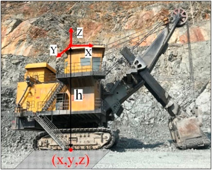
Figure 1. Position measurement during movement of the electric shovel.

As shown in Figure 2, the data acquisition system was installed on an electric shovel in an open-pit mine to monitor the coordinate data of the bench floor, including four feature vectors: longitude (X), dimension (Y), elevation (Z), and time (T). In order to quantitatively evaluate the terrain of the bench floor, it was difficult to construct the global bench floor DEM at the one time. In this study, according to the continuity and spatial distribution characteristics of data acquisition over time, six groups of representative regions with varying terrains were selected for research during the operational period of the electric shovel. Table 1 presents the statistical information of the data, including the number of points, elevation range and standard deviation, and the average distance between the discrete points.

Figure 2

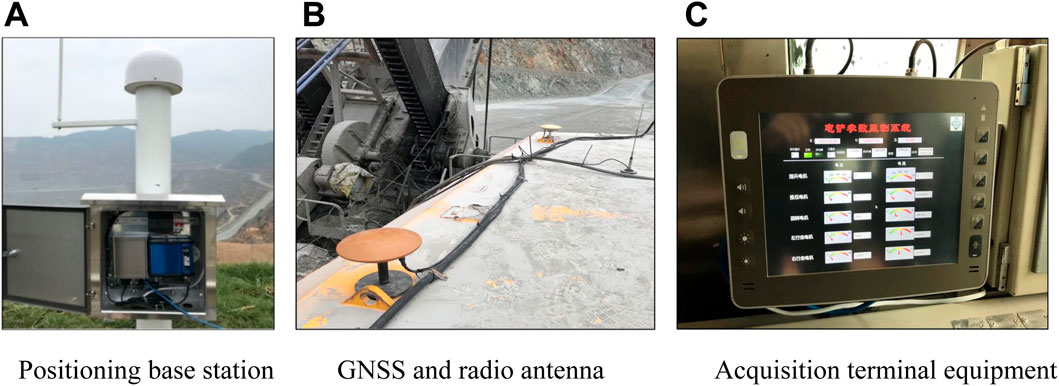
Figure 2. Data acquisition system based on RTK-GNSS positioning. (A) Positioning base station. (B) GNSS and radio antenna. (C) Acquisition terminal equipment.

Table 1

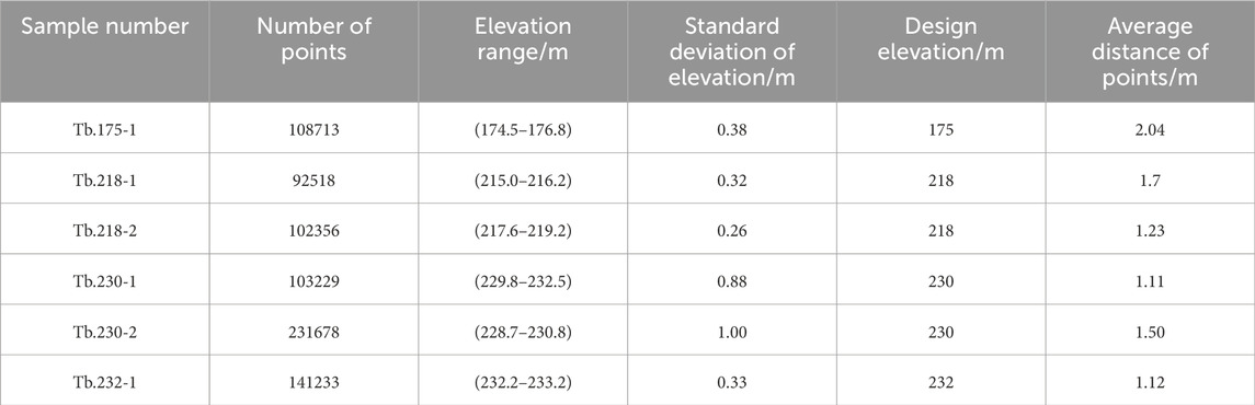
Table 1. Collection information on the datasets.

2.2 Materials and methods

The Python programming language was utilized for analysis of the monitoring data, incorporating algorithms such as discrete points boundary identification, interpolation, and terrain factor calculation. Figure 3 shows the DEM modeling analysis process of the bench floor. First, the discrete points identification boundary algorithm is introduced to delineate the research area of the bench floor. Second, the discrete points in the effective region are randomly divided into two parts: 80% training sets and 20% test sets. Third, various algorithms are employed to interpolate the training sets within the study area, leading to a discussion on the errors in the DEM generated by different algorithms. Furthermore, an analysis is conducted on the impact of interpolation parameters, data density, the terrain characteristics of the interpolation methods, ultimately culminating in the selection of the optimal interpolation algorithm. Finally, the relevant parameters and indices of describing the bench floor are calculated based on DEM model.

Figure 3

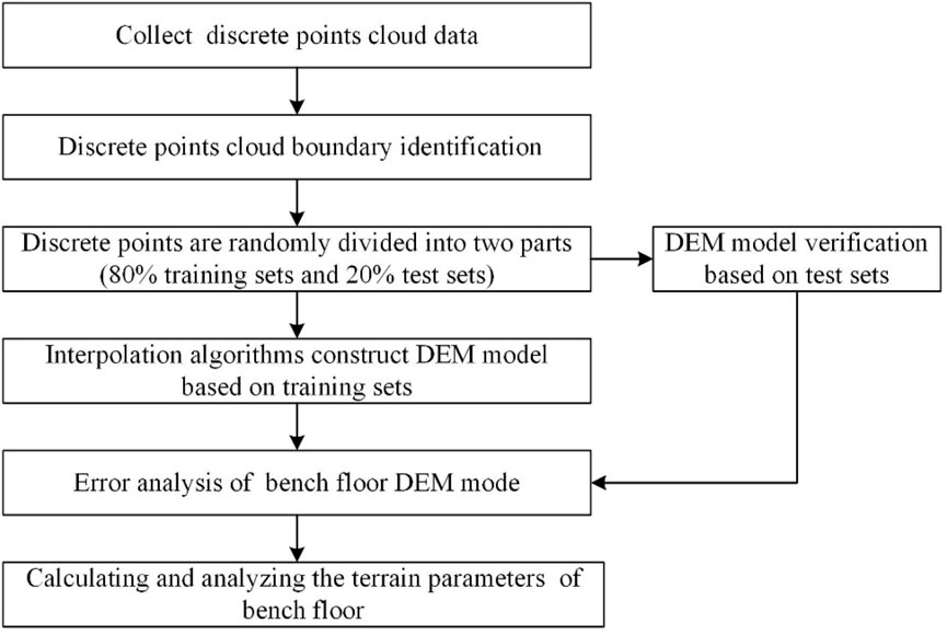
Figure 3. DEM modeling analysis process of the bench floor.

2.2.1 Discrete point boundary extraction algorithm

This study proposes an improved algorithm that can automatically extract the optimal boundary of an arbitrary point distribution based on the convex hull model algorithm (Qian and Liu, 2007; Liu et al., 2011; Yang, 2021). In the improved algorithm, the α-shape algorithm which automatically adjusts the 2α value is used to extract the boundary in the two-dimensional mesh. Figure 4 shows the process of extracting the boundary.

Figure 4

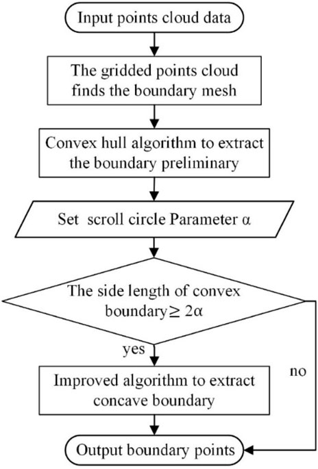
Figure 4. Flowchart of the point cloud boundary extraction algorithm.

Coordinate points are projected onto a two-dimensional plane along the Z-axis, maintaining the X and Y values. The neighborhood grid point detection method determines the internal and boundary grids. Hengl demonstrated that the optimal DEM grid resolution should be half the average point distance (Heng, 2006). Therefore, the size of the grid should be set to half the average distance of the points.

The vertical lines of the x and y-axes were drawn according to the boundary grid points to generate rectangular bounding boxes. The discrete points in the non-boundary grid were excluded by triangular meshing in the inner point cloud of the rectangular region, and the discrete points in the boundary grid were identified using the convex hull algorithm (He et al., 2023). Figure 5A shows an example of a minimum convex algorithm. The minimum rectangular bounding box (A-B-C-D) is first determined; subsequently, the uppermost point $y_{\mathit{max}}$ and the lowest point $y_{\mathit{min}}$ are connected. The rectangular bounding box is divided into left and right parts. On the left side of the data, the top, bottom, and leftmost points are connected to each line segment; points a and b are furthest from the outside of the line segment and connect a to $y_{\mathit{max}}$, a to $x_{\mathit{min}}$, b to $y_{\mathit{min}}$, and b to $x_{\mathit{min}}$, respectively. The same method was applied to the four lines formed by points a and b, and all boundary points of the left half were found in turn. The right half of the data is processed according to the same method. The algorithm is capable of effectively extracting the minimum convex deformation boundary; however, it cannot concave the boundary.

Figure 5

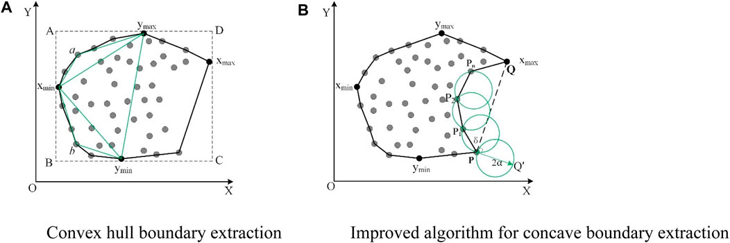
Figure 5. Simulated point cloud and its boundary extraction. (A) Convex hull boundary extraction. (B) Improved algorithm for concave boundary extraction.

The proposed improved algorithm was used to extract the point cloud concave boundary. It sets 2α based on the convex boundary segment lengths. Shorter lengths indicate adjacent points, while longer lengths suggest non-adjacent points. Therefore, the quartile of each length value of the convex boundary line is counted. The value of 2α is determined as the highest quartile. Subsequently, the concave boundary points are extracted. Concave boundaries are then found where convex boundary lengths exceed 2α, using the α-shape algorithm.

As shown in Figure 5B, First, the α-shape algorithm is used when line segment $\mathrm{P}\mathrm{Q}>2\mathrm{\alpha }$. A circle with ${\text{PQ}}^{\prime }$ as its diameter is rolled counterclockwise from P to Q ($\left|{\mathrm{P}\mathrm{Q}}^{\prime }\right|=2\mathrm{\alpha }$, ${\mathrm{P}\mathrm{Q}}^{\prime }\perp PQ$). When the first point is P₁ in the 2α neighborhood, calculate the modulus of P₁Q. If ${\mathrm{P}}_1\mathrm{Q}>2\mathrm{\alpha }$ is still true, the next point P₂ is found according to the above method. Repeat the process until Pn is found where ${\mathrm{P}}_n\mathrm{Q}\le 2\mathrm{\alpha }$ at which point the process stops. Finally, the optimal boundary is found by connecting all the boundary points in turn.

2.2.2 Interpolation method

Spatial interpolation transforms spatially continuous points into continuous data surfaces (Mao, 2007; Tang, 2014; Huang et al., 2023). Five interpolation methods (IDW, RBF, TIN, NN, and OK) were selected for DEM construction, with a comparative analysis conducted to evaluate accuracy and factors affecting interpolation errors.

(1) Interpolation method

The IDW calculated the weighted average using the distance between the sampling point and the interpolation point as the weight. The IDW interpolation is expressed as Eq. 1 (Achilleos, 2008):

$\mathit{f}\left(\mathit{x},\mathit{y}\right)=\frac{{\displaystyle {\sum }_{\mathit{i}=\mathbf{1}}^{\mathit{n}}}\frac{{\mathit{z}}_{\mathit{i}}}{{\mathit{d}}_{\mathit{i}}^{\mathit{p}}}}{{\displaystyle {\sum }_{\mathit{i}=\mathbf{1}}^{\mathit{n}}}\frac{\mathbf{1}}{{\mathit{d}}_{\mathit{i}}^{\mathit{p}}}},(1)$

where $f\left(x,y\right)$ is the elevation value of the point to be measured, $n$ is the number of sample points, $z_i$ is the elevation value of the $ith$ sample point, $d_i$ is the Euclidean distance from the measured to the sample point, and $p$ is a power with a value in the range of 1–3.

The RBF is more appropriate for computing homologous spatial interpolations. RBF established in Eq. 2:

$\mathit{f}\left(\mathit{x},\mathit{y}\right)={\displaystyle {\sum }_{\mathit{i}=\mathbf{1}}^{\mathit{n}}}{\mathit{\alpha }}_{\mathit{i}}\mathit{\phi }\left({‖\mathit{x}-{\mathit{x}}_{\mathit{i}}‖}_{\mathbf{2}}\right),(2)$

where $\phi \left({‖x-x_i‖}_2\right)$ is the radial basis function, ${‖x-x_i‖}_2$ is the Euclidean distance from the point to be interpolated to the sampling point, ${\alpha }_i$ is the interpolation coefficient, and n neighborhood points are searched by reference to a kd-tree (Zhou et al., 2008).

The TIN builds triangles using a sequence of points (Cao et al., 2014). However, it has the disadvantage that there may be sudden changes in the edge gradient (Li and Heap, 2014).

The NN is based on the mesh division within the sample region, and attribute values of the mesh vertices and interior are obtained using the linear interpolation method (Mao, 2007).

The OK is a geostatistical method that uses the variance function as weights to unbiased optimal estimation. The OK interpolation method uses the variation function to express the spatial variation (Anderson et al., 2006; Viswanathan et al., 2015; Hekmatnejad et al., 2019), according to Eq. 3:

$\mathit{f}\left(\mathit{x},\mathit{y}\right)={\displaystyle {\sum }_{\mathit{i}=\mathbf{1}}^{\mathit{n}}}{\mathit{\lambda }}_{\mathit{i}}{\mathit{z}}_{\mathit{i}},(3)$

where ${\lambda }_i$ is the weight coefficient. The weight coefficients can be obtained by the theoretical variogram model. The variogram model and its related parameters (nugget value, variation range, and partial base value) are key factors that affect the interpolation accuracy (Zhang, 2014). Variogram function models include spherical, Gaussian, and exponential model (Zhang et al., 2022b). It is crucial to select a reasonable theoretical variogram function model and parameters for simulation accuracy. First, semi-variance values for different lag distances are calculated using the sample data, leading to the construction of an experimental variogram. The chart illustrates the spatial correlation of the sample data as distance varies. Second, the best model describing the spatial structure of data is selected based on the experimental value. Third, the nugget, range, and sill of the theoretical variogram model are estimated using the nonlinear least squares fitting method. It is necessary to evaluate the degree of fit by observing the residual, calculating the fitting coefficient, or comparing graphs.

(2)Data density

Due to the presence of duplicate and null values in the original data, the study area is divided into grids of equal spacing. Duplicate data points within each grid were filtered to retain the mean value. The maximum sampling rate is defined as the ratio of the number of original samples to the total number of grids.

The error of DEM is constructed by different density point clouds. The training data is set down to the grid resolution under densities of 70%, 60%, 50%, 40%, 30%, 20%, and 10%. The amount of extracted data is shown in Table 2.

(3) Error evaluation

Table 2

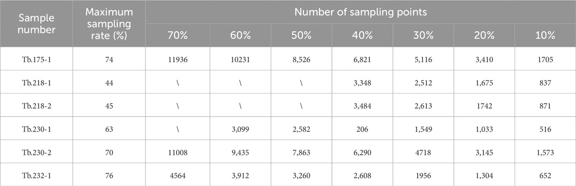
Table 2. Number of sample points after data reduction.

Some test data are used to verify DEM accuracy. Grid elevation values from the DEM are extracted at verification point locations. Based on the extracted grid elevation values and the corresponding verification point’s elevation values, the error index is calculated, and the error of the interpolation algorithm is evaluated.

The root mean square error (RMSE), calculated as Eq. 4, and goodness of fit (R²), calculated as Eq. 5, methods are selected as error evaluation indices. When the RMSE value is smaller or R² is closer to 1, the error of the DEM simulation is optimal.

$\mathbf{\text{RMSE}}=\sqrt{\frac{\mathbf{1}}{\mathbf{n}}{\displaystyle {\sum }_{\mathbf{i}=\mathbf{1}}^{\mathbf{n}}}{\left({\mathbf{Z}}_{\mathbf{i}}-\widehat{{\mathbf{Z}}_{\mathbf{i}}}\right)}^{\mathbf{2}}},(4)$

${\mathbf{R}}^{\mathbf{2}}=\mathbf{1}-\frac{{\displaystyle {\sum }_{\mathbf{i}=\mathbf{1}}^{\mathbf{n}}}{\left({\mathbf{Z}}_{\mathbf{i}}-\widehat{{\mathbf{Z}}_{\mathbf{i}}}\right)}^{\mathbf{2}}}{{\displaystyle {\sum }_{\mathbf{i}=\mathbf{1}}^{\mathbf{n}}}{\left({\mathbf{Z}}_{\mathbf{i}}-\overline{{\mathbf{Z}}_{\mathbf{i}}}\right)}^{\mathbf{2}}},(5)$

where $\widehat{{\mathrm{Z}}_{\mathrm{i}}}$ is the predicted value, ${\mathrm{Z}}_{\mathrm{i}}$ is the truth value, n is the number of samples used to validate the test sets, and $\overline{Z_i}$ is the average elevation.

2.2.3 Terrain parameters

In order to quantitatively analyze the roughness of the bench floor, three evaluation indexes are defined as regional area, surface slope, and roughness.

(1) Regional area

The set boundary coordinates are [$\left(x_i,y_i\right),i=1,2\cdots ,n$], and $n$ is the number of boundary points. The regional area is expressed as:

${\mathit{S}}_{\mathbf{1}}=\frac{\mathbf{1}}{\mathbf{2}}{\displaystyle {\sum }_{\mathit{i}=\mathbf{1}}^{\mathit{n}-\mathbf{1}}}\left({\mathit{x}}_{\mathit{i}+\mathbf{1}}+{\mathit{x}}_{\mathit{i}}\right)·\left({\mathit{y}}_{\mathit{i}+\mathbf{1}}-{\mathit{y}}_{\mathit{i}}\right).(6)$

(2) Surface slope

Assuming that the fitting slope equation could be written as $\mathrm{Z}=\text{AX}+\text{BY}+\mathrm{D}$, the coefficients A, B, and D were obtained by using the least-squares method to fit the interpolated data. The surface slope ($\mathrm{\theta }$) is calculated thus:

$\mathit{\theta }=\mathbf{tan}\left(\mathit{arccos}\frac{\mathbf{1}}{\sqrt{{\mathit{A}}^{\mathbf{2}}+{\mathit{B}}^{\mathbf{2}}+\mathbf{1}}}\right).(7)$

(3) Surface roughness

Surface roughness refers to the degree of deviation between real and ideal surfaces in the vertical direction. The standard deviation of the vertical distance from each point to the fitting surface is calculated as $S_d$. If $S_d$ is smaller, the roughness is smaller.

The vertical distance from each point $\left(x_i,y_i,z_i\right)$ to the fitting surface after interpolation is expressed as follows:

${\mathit{d}}_{\mathit{i}}=\frac{\left|\mathit{A}{\mathit{x}}_{\mathit{i}}+\mathit{B}{\mathit{y}}_{\mathit{i}}+\mathit{D}-{\mathit{z}}_{\mathit{i}}\right|}{\sqrt{{\mathit{A}}^{\mathbf{2}}+{\mathit{B}}^{\mathbf{2}}+\mathbf{1}}}.(8)$

All points on the fitting surface $\overline{d}$ have a vertical distance average and standard deviation $S_d$ such that

$\overline{\mathit{d}}=\frac{\mathbf{1}}{\mathit{K}}{\displaystyle {\sum }_{\mathit{i}=\mathbf{1}}^{\mathit{K}}}{\mathit{d}}_{\mathit{i}},(9)$

${\mathit{S}}_{\mathit{d}}=\sqrt{\frac{{\displaystyle {\sum }_{\mathit{i}=\mathbf{0}}^{\mathit{K}}}{\left({\mathit{d}}_{\mathit{i}}-\overline{\mathit{d}}\right)}^{\mathbf{2}}}{\mathit{K}-\mathbf{1}}.}(10)$

The overcut or undercut areas can be used for terrain indexes. These areas are determined by judging whether the distance ($d_i$) from each point to the fitting surface exceeds the threshold range ∆d (∆d=0.3 m). s_grid is the size of the model grid.

$\left\{\begin{array}{c}{\mathbf{S}}_{\mathit{c}}={\displaystyle {\sum }_{\mathit{i}=\mathbf{1}}^{\mathit{m}}}{\mathit{d}}_{\mathit{i}}·{\mathit{s}}_{\mathit{g}\mathit{r}\mathit{i}\mathit{d}}\mathbf{i}\mathbf{f}{\mathit{d}}_{\mathit{i}}<-∆\mathit{d}\\ {\mathbf{S}}_{\mathit{o}}={\displaystyle {\sum }_{\mathit{i}=\mathbf{1}}^{\mathit{m}}}{\mathit{d}}_{\mathit{i}}·{\mathit{s}}_{\mathit{g}\mathit{r}\mathit{i}\mathit{d}}\mathbf{i}\mathbf{f}{\mathit{d}}_{\mathit{i}}\le \left|∆\mathit{d}\right|\\ {\mathbf{S}}_{\mathit{q}}={\displaystyle {\sum }_{\mathit{i}=\mathbf{1}}^{\mathit{m}}}{\mathit{d}}_{\mathit{i}}·{\mathit{s}}_{\mathit{g}\mathit{r}\mathit{i}\mathit{d}}\mathbf{i}\mathbf{f}{\mathit{d}}_{\mathit{i}}>+∆\mathit{d}\end{array}\right..(11)$

3 Results and discussion

3.1 Interpolation algorithm parameters

Parameters of the interpolation algorithms were considered as follows: the power of the IDW was set to 2, and 30 adjacent points were searched. The RBF used a Gaussian RBF to search for 30 adjacent points. The TIN constructed triangular mesh for linear interpolation. Parameters of the OK were obtained through fitting the experiment and theoretical variance functions from each sample data. The fitting process utilized the nonlinear least squares method, iteratively adjusting the model parameters to minimize the differences between the theoretical and experimental variograms. Consequently, the range, sill, and nugget of the theoretical variograms were determined through this iterative refinement process.

Theoretical variogram models such as the Gaussian, exponential, and spherical models are selected based on the experimental variogram graph. As shown in Figure 6, the scatter of the experimental variation function and the curve of the theoretical variation function were fitted. The fitting coefficients (R²) for the spherical, Gaussian, and exponential models are 0.968, 0.937, and 0.899, respectively. The optimal variogram model is the spherical model, its range β, nugget value $C_0$, and range value $C$ being 106, 0.02, and 0.192, respectively.

Figure 6

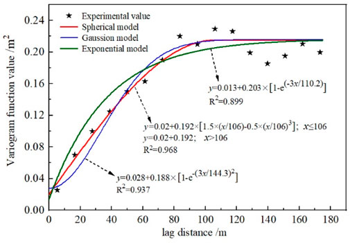
Figure 6. Experimental and theoretical variogram models of Tb.175-1.

3.2 DEM of the bench floor

Taking the Tb.175-1 as a case (Figure 7), the visualization effects of different interpolation algorithms to simulate bench floor DEM are compared. The DEMs from five interpolation algorithms fill gaps and capture terrain trends yet differ markedly in visual quality. In Figure 8A, the IDW is easily affected by the density of extreme points. Enhancing the sample count improves terrain detail retention. In the cavity regions, the interpolation outcomes were similar, resulting in a smooth surface influenced by neighboring points. In Figure 8B, the surface is not continuous and smooth, and the fluctuation phenomenon at the boundary position is especially significant. In Figure 8C, TIN adopts linear interpolation to generate multiple abnormal “step” surfaces in the dotted cavity area, which is completely different from the real bench floor terrain. The NN (Figure 8D) offers smoothness in uniformly sampled areas but generates a “sawtooth” edge effect where samples are lacking. The OK (Figure 8E) considers global points distribution in the interpolation calculation of terrain in the void and nonuniform scattered areas, delivering a smooth DEM that accurately delineates terrain undulations and effectively reflects local variations.

Figure 7

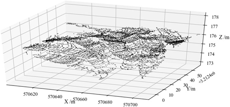
Figure 7. Distribution of original discrete points.

Figure 8

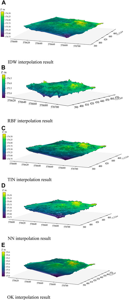
Figure 8. DEM results of different interpolation methods. (A) IDW interpolation result. (B) RBF interpolation result. (C) TIN interpolation result. (D) NN interpolation result. (E) OK interpolation result.

After comparing the DEM results, the accuracy of each interpolation method is verified by using the truth value on the simulated elevation data. As shown in Figure 9, the desired value (black line) indicates that the estimated value is the same as the truth value. The distance between the estimated value of each algorithm and the black line segment indicates the error value.

Figure 9

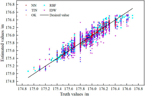
Figure 9. Verification of the truth and estimated values of Tb.175-1 elevation.

The weight value of the OK interpolation optimizes continuity and smoothness by considering the distance between the interpolation and sampling points and their spatial distribution relationship. Conversely, other algorithms have limited weights, resulting in poor simulation results in blind areas and edges.

3.3 DEM error of different interpolation methods

3.3.1 Data density factor

By studying the variations in RMSE values at different data densities, we aim to uncover the performance of DEM interpolation methods in the Tb.175-1 area and understand the impact of data density on DEM error.

Figure 10 shows the RMSE of five interpolation methods as influenced by data density. Increasing data density leads to a gradual RMSE reduction before stabilization. Notably, RBF is less affected by lower data density (<40%). However, RMSE values exceed 0.2 m for all algorithms between 10% and 40% density. IDW is notably sensitive to sampling density in terrain fluctuating areas. Between 40% and 60% density, errors decrease notably, with NN showing the largest reduction (0.27 m–0.154 m) and TIN the smallest (0.24m–0.15 m). Above 60% density, errors plateau below 0.2 m, indicating minimal impact on DEM accuracy. This shows that the interpolation methods have less influence on DEM accuracy when data density is larger. The maximum sampling rate of TB175-1 is 74% of the whole grid due to the reduction of sampling data and sampling blind area. At the maximum sampling rate, the RMSE values for OK, RBF, IDW, TIN and NN are 0.101 m, 0.13 m, 0.144 m, 0.152 m, and 0.156 m, respectively.

Figure 10

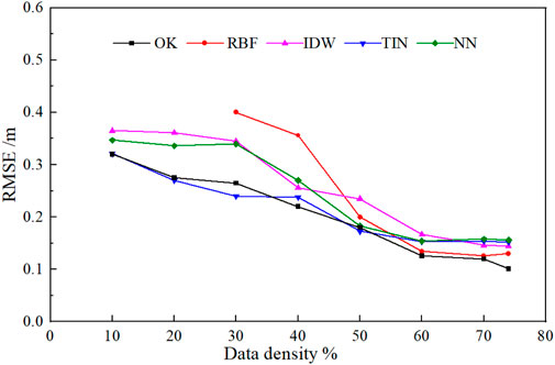
Figure 10. RMSE of the algorithm for different data densities.

3.3.2 Regional terrain factor

The DEM errors of six test areas were compared and analyzed under the maximum sampling rate. As shown in Figure 11, OK interpolation demonstrates the highest accuracy, with an RMSE below 0.22 m and R² exceeding 0.909 for the same sample data. Conversely, IDW exhibits the largest RMSE, with three test areas (Tb.218-1, Tb.218-2, and Tb.230-2) exceeding 0.32 m and R² below 0.853. Based on the algorithm’s principle, IDW estimates cannot surpass the elevation range of sampling points, leading to significant errors in terrain with limited sampling. RBF, TIN, and NN algorithms show similar RMSE values, with consistent trends across all samples.

Figure 11

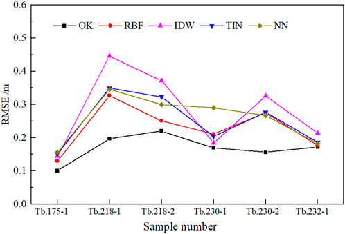
Figure 11. RMSE of DEM-generated different interpolation algorithms.

The overall variation trend of DEM error is positively correlated with surface roughness. For example, the RMSE of the DEM errors in Tb.218-1 considering roughness are highly significant. Therefore, when the floor is very rough, the number of samples should be increased to the highest possible extent to enhance the terrain detail retention ability and reduce interpolation errors.

The above analysis shows the following. 1) The interpolation algorithms can be ranked according to RMSE values, from smallest to largest: OK, TIN, RBF, NN, and IDW. 2) When the sampling density is low, IDW shows the highest error while RBF exhibits the lowest. For sampling rates exceeding 60%, all five interpolation methods demonstrate minimal errors, showcasing good robustness. 3) OK is least impacted by terrain features when sampling density requirements are met. Therefore, the optimal OK interpolation yields the minimum accuracy error RMSE, which is close to that of the real surface.

3.4 Analysis of bench floor terrain

The DEMs were established using the OK interpolation algorithm. As shown in Figure 12A−F, contour maps are visualized for the floor terrain.

Figure 12

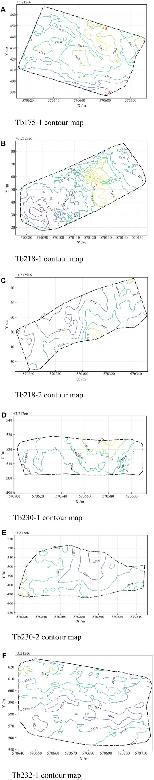
Figure 12. Simulation results of the bench floor contour map. (A) Tb175-1 contour map. (B) Tb218-1 contour map. (C) Tb218-2 contour map. (D) Tb230-1 contour map. (E) Tb230-2 contour map. (F) Tb232-1 contour map.(a)(b)

According to Eqs (6–11), the bench floor terrain parameters are calculated as shown in Table 3. The average slope of the bench floor in six test areas is 1.34%, with an average roughness of 0.21 m and average undercut rate approximately three-times higher than the overcut rate. The presence of concave and convex terrain on the bench floor locally obstructs the digging operation of the electric shovel bucket, impacting efficiency of transportation by electric wheels. In particular, the undercut rates of Tb175-1 and Tb218-2 exceed the average, reaching 20.61%, 24.68%, and 18.86%, respectively. This higher undercut rate post-blasting may be the underlying cause of the challenges faced during shovel digging operations. Moreover, the overall slope of Tb230-1 exceeds the average value by 3.41%, and Figure 12D depicts a significant elevation difference between the highest and lowest points of the bench floor DEM; the standard deviation of the actual elevation at 0.88 indicates unfavorable conditions for subsequent vertical drilling activities. The local roughness of the Tb.218-1 is 0.39 m, highlighting the undulating terrain.

Table 3

Table 3. Calculation results of terrain parameters of the bench floor.

4 Conclusion

To meet the practical demands of production management in open-pit mines, this study proposes a method for assessing the terrain of the bench floor. The conclusions as follows:

(1) An optimized convex hull boundary recognition algorithm is proposed. The algorithm automatically determines the boundary of discrete points and determines the valid interpolation region for the DEM.

(2) Considering the influence of sampling data density and terrain features on the accuracy of different interpolation algorithms, the results show that DEM errors decrease gradually and tend to be stable with increased sampling density. For complex terrain features, the accuracy of DEM can be improved by increasing the sampling density to more than 60%. The general terrain features can reduce the number of samples appropriately to improve calculation efficiency.

(3) By comparing the terrain quality on the bench floor achieved by five interpolation algorithms, it is observed that the OK interpolation algorithm can fill the holes of the original points. This resulted in smoother DEMs with enhanced visualization effects. In this study, the theoretical variogram and related parameters of OK interpolation were determined by the algorithm fitting. It improved the accuracy of the DEM, minimizing fluctuations in RMSE values.

(4) The digital quantification index of the roughness of the bench floor is established. These parameters offer essential data for mining technologists, enabling them to assess the blasting effects and implement refined management practices for bench floor leveling operations.

Data availability statement

The original contributions presented in the study are included in the article/supplementary material; further inquiries can be directed to the corresponding author.

Author contributions

BW: data curation and writing–original draft. BG: investigation and writing–review and editing. WX: formal analysis and writing–review and editing. XS: conceptualization, methodology, and writing–review and editing.

Funding

The author(s) declare that financial support was received for the research, authorship, and/or publication of this article. This research was funded by the Major Scientific Program of Jiangxi Copper Co., Ltd., grant number (No. DTYJ201800), the Scientific Program of Baotou Steel Union Co., Ltd., grant number (No. 202107), and the Innovation and Entrepreneurship Science and Technology Special Project of Coal Research Institute (No. 2021-KXYJ-002). The authors declare that this study received funding from Jiangxi Copper Co., Ltd. and Baotou Steel Union Co., Ltd. The funders were not involved in the study design, collection, analysis, interpretation of data, the writing of this article, or the decision to submit it for publication.

Acknowledgments

The authors gratefully acknowledge the technical support provided by the Beijing General Research Institute of Mining and Metallurgy. They thank Jiangxi Dexing Copper Mine Co., Ltd. for its test equipment.

Conflict of interest

The authors declare that the research was conducted in the absence of any commercial or financial relationships that could be construed as a potential conflict of interest.

Publisher’s note

All claims expressed in this article are solely those of the authors and do not necessarily represent those of their affiliated organizations, or those of the publisher, the editors, and the reviewers. Any product that may be evaluated in this article, or claim that may be made by its manufacturer, is not guaranteed or endorsed by the publisher.

References

Achilleos, G. (2008). Errors within the inverse distance weighted (IDW) interpolation procedure. Geocarto Int. 23, 429–449. doi:10.1080/10106040801966704

CrossRef Full Text | Google Scholar

Aguilar, F. J., Agüera, F., Aguilar, M. A., and Carvajal, F. (2005). Effects of terrain morphology, sampling density, and interpolation methods on grid DEM accuracy. Photogrammetric Eng. Remote Sens. 71, 805–816. doi:10.14358/pers.71.7.805

CrossRef Full Text | Google Scholar

Aguilar, F. J., Aguilar, M. A., Agüera, F., and Sanchez, J. (2006). The accuracy of grid digital elevation models linearly constructed from scattered sample data. Int. J. Geogr. Inf. Sci. 20, 169–192. doi:10.1080/13658810500399670

CrossRef Full Text | Google Scholar

Anderson, E. S., Thompson, J. A., Crouse, D. A., and Austin, R. E. (2006). Horizontal resolution and data density effects on remotely sensed LIDAR-based DEM. Geoderma 132, 406–415. doi:10.1016/j.geoderma.2005.06.004

CrossRef Full Text | Google Scholar

Bater, C. W., and Coops, N. C. (2009). Evaluating error associated with lidar-derived DEM interpolation. Comput. Geosciences 35, 289–300. doi:10.1016/j.cageo.2008.09.001

CrossRef Full Text | Google Scholar

Cao, L., Zhu, X. Z., and Dai, J. S. (2014). Error analysis of DEM interpolation based on small-foolprint airborne lidar in subtropical hilly forest. J. Nanjing For. Univ. Nat. Sci. Ed. 38, 7–13. doi:10.3969/j.issn.1000-2006.2014.04.002

CrossRef Full Text | Google Scholar

Chen, C., Li, Y., Zhao, N., Guo, B., and Mou, N. X. (2018). Least squares compactly supported radial basis function for digital terrain model interpolation from airborne lidar point clouds. Remote Sens. 10, 587–611. doi:10.3390/rs10040587

CrossRef Full Text | Google Scholar

Chu, H. J., Wang, C. K., Huang, M.-L., Lee, C. C., Liu, C. Y., and Lin, C. C. (2014). Effect of point density and interpolation of LiDAR-derived high-resolution DEMs on landscape scarp identification. GIS Sci. Remote Sens. 51, 731–747. doi:10.1080/15481603.2014.980086

CrossRef Full Text | Google Scholar

Duan, Y., Xiong, D. Y., and Xu, G. Q. (2015). A new technology for digital drilling and automatic lithology identification. Metal. Mine 10, 125–129.

Google Scholar

Erdogan, S. A. (2009). A comparision of interpolation methods for producing digital elevation models at the field scale. Earth Surf. Process. Landforms 34, 366–376. doi:10.1002/esp.1731

CrossRef Full Text | Google Scholar

Fan, P., Li, W., Cui, X., and Lu, M. (2019). Precise and robust RTK-GNSS positioning in urban environments with dual-antenna configuration. Sensors 19 (16), 3586. doi:10.3390/s19163586

PubMed Abstract | CrossRef Full Text | Google Scholar

Fang, X. J. (2019). Construction and implementation of high-precision solution model for surface deformation monitoring in mining area based on GPS/BDS combination. Huainan, China: AnHui University of Science and Technology.

Google Scholar

Gao, Y., Zhu, Y., Chen, C. F., Hu, Z. Z., and Hu, B. J. (2021). A weighted radial basis function interpolation method for high accuracy DEM modeling. Geomatics Inf. Sci. Wuhan Univ., 1–9. doi:10.13203/j.whugis20210100

CrossRef Full Text | Google Scholar

Guo, Q., Li, W., Yu, H., and Otto, A. (2010). Effects of topographic variability and lidar sampling density on several DEM interpolation methods. Photogrammetric Eng. Remote Sens. 76, 701–712. doi:10.14358/pers.76.6.701

CrossRef Full Text | Google Scholar

He, X., Wang, R., Feng, C., and Zhou, X. Q. (2023). A novel type of boundary extraction method and its statistical improvement for unorganized point clouds based on concurrent delaunay triangular meshes. Sensors 23, 1915–1923. doi:10.3390/s23041915

PubMed Abstract | CrossRef Full Text | Google Scholar

Hekmatnejad, A., Emery, X., and Alipour-Shahsavari, M. (2019). Comparing linear and non-linear kriging for grade prediction and ore/waste classification in mineral deposits. Int. J. Min. Reclam. Environ. 33, 247–264. doi:10.1080/17480930.2017.1386430

CrossRef Full Text | Google Scholar

Heng, L. T. (2006). Finding the right pixel size. Comput. Geosciences 32, 1283–1298. doi:10.1016/j.cageo.2005.11.008

CrossRef Full Text | Google Scholar

Huang, F. M., Huang, J. S., Jiang, S. H., and Zhou, C. B. (2017). Landslide displacement prediction based on multivariate chaotic model and extreme learning machine. Eng. Geol. 218, 173–186. doi:10.1016/j.enggeo.2017.01.016

CrossRef Full Text | Google Scholar

Huang, F. M., Xiong, H. W., Yao, C., Catani, F., Zhou, C. B., and Huang, J. S. (2023). Uncertainties of landslide susceptibility prediction considering different landslide types. J. Rock Mech. Geotechnical Eng. 15, 2954–2972. doi:10.1016/j.jrmge.2023.03.001

CrossRef Full Text | Google Scholar

Huang, F. M., Zhang, J., Zhou, C. B., Wang, Y. H., Huang, J. S., and Zhu, L. (2020). A deep learning algorithm using a fully connected sparse autoencoder neural network for landslide susceptibility prediction. Landslides 17, 217–229. doi:10.1007/s10346-019-01274-9

CrossRef Full Text | Google Scholar

Jing, Y. P., Liu, G., and Jin, Z. K. (2019). GNSS antenna combined with AHRS measurement of field topography. Agric. Eng. J. 35, 166–174. doi:10.11975/j.issn.1002-6819.2019.21.020

CrossRef Full Text | Google Scholar

Li, H. P., Niu, D. L., and Wang, Y. (2014). Rapid survey technology of farmland terrain based on RTK GNSS. J. China Agric. Univ. 19, 188–194. doi:10.11841/j.issn.1007-4333.2014.06.26

CrossRef Full Text | Google Scholar

Li, J., and Heap, A. D. (2014). Spatial interpolation methods applied in the environmental sciences: a review. Environ. Model. Softw. 53, 173–189. doi:10.1016/j.envsoft.2013.12.008

CrossRef Full Text | Google Scholar

Liu, R. W., Yang, D. H., Li, Y., and Chen, K. (2011). An improved algorithm for producing minmun convex hull. J. Geodesy Geodyn. 31, 130–133. doi:10.14075/j.jgg.2011.03.003

CrossRef Full Text | Google Scholar

Lv, H. Y., Sheng, Y. H., Duan, P., Zhang, S. Y., and Li, J. (2015). A hierarchical RBF interpolation method based on local optimal shape parameters. J. Geo-information Sci. 17, 260–267. doi:10.3724/SP.J.1047.2015.00260

CrossRef Full Text | Google Scholar

Mao, D. Z. (2007). Study on the construction method of TIN model. Nanjing, China: Huhai University.

Google Scholar

Meng, Z. J., Fu, W. Q., and Liu, H. (2009). Design and implementation of 3D topographic surveying system in vehicle for field precision leveling. Trans. Chin. Soc. Agric. Eng. 25, 255–259. doi:10.3969/j.issn.1002-6819.2009.z2.049

CrossRef Full Text | Google Scholar

Montealegre, A., Lamelas, M., and Riva, J. (2015). Interpolation routines assessment in ALS-derived digital elevation models for forestry applications. Remote Sens. 7, 8631–8654. doi:10.3390/rs70708631

CrossRef Full Text | Google Scholar

Qian, Z., and Liu, R. T. (2007). An improved incremental algorithm for determining the convex hull of A set of points. Heilongjiang, China: Harbin university of Science and Technology.

Google Scholar

Shen, J., Su, T. Y., Wang, G. Y., Liu, H. X., and Li, J. G. (2012). Submarine topography visualization based on kriging algorithm. Mar. Sci. 36, 24–28.

Google Scholar

Tang, G. A. (2014). Progress of DEM and digital terrain analysis in China. Acta Geogr. Sin. 69, 1305–1325. doi:10.11821/dlxb201409006

CrossRef Full Text | Google Scholar

Viswanathan, R., Jagan, J., Samui, P., and Porchelvan, P. (2015). Spatial variability of rock depth using simple kriging, ordinary kriging, RVM and MPMR. Geotechnical Geol. Eng. 33, 69–78. doi:10.1007/s10706-014-9823-y

CrossRef Full Text | Google Scholar

Wang, C. R. (2020). Application of GNSS technology in mine survey. Nat. Resour. North China 3, 85–86.

Google Scholar

Wang, P., Feng, D. W., Chen, G. L., He, J., Hu, L., and Peng, J. Y. (2023). Real-time 3D terrain measurement method and experiment in farmland leveling. Agric. Mach. J. 54, 41–48. doi:10.6041/j.issn.1000-1298.2023.03.004

CrossRef Full Text | Google Scholar

Wei, D., Chen, M., Lu, W. B., Li, K. G., and Wang, G. H. (2022). Formation mechanism of blasting tight bottom caused by lithologic change. Rock Soil Mech. 43 (S1), 490–500. doi:10.16285/j.rsm.2021.0147

CrossRef Full Text | Google Scholar

Yang, H. W. (2021). Accelerating algorithm for convex hull construction of 2D scattered point cloud. Chin. J. Electron. 34, 55–60. doi:10.16576/j.cnki.1007-4414.2021.02.016

CrossRef Full Text | Google Scholar

Yokota, M., Mizushima, A., and Ishii, K. (2004). 3D map generation by A robot tractor equipped with A laser range finder. Automation Technol. Off-Road Equip., 374–379. doi:10.13031/2013.17855

CrossRef Full Text | Google Scholar

Zhang, B., Liu, Q., Xu, g. L., Cai, R. L., and Cheng, F. (2022a). Application of GNSS+INS integrated navigation in mine auto-driving trucks. Bull. Surv. Mapp. 7, 143–147. doi:10.13474/j.cnki.11-2246.2022.0219

CrossRef Full Text | Google Scholar

Zhang, J. (2014). Interpolation of point clouds data based on kriging interpolation. Xi'an, China: Chang’an University.

Google Scholar

Zhang, Q., Ma, Y. N., Wang, X. J., Shen, Y. X., and Yi, W. J. (2022b). Modeling of main discontinuities of rock tunnel based on optimized kriging interpolation method. China Civ. Eng. J. 55, 74–82. doi:10.15951/j.tmgcxb.2022.s2.07

CrossRef Full Text | Google Scholar

Zhou, K., Hou, Q., Wang, R., and Guo, B. N. (2008). Real-time KD-tree construction on graphics hardware. ACM Trans. Graph. 27, 1–11. doi:10.1145/1409060.1409079

CrossRef Full Text | Google Scholar