Deep learning-based spatial downscaling and its application for tropical cyclone detection in the western North Pacific

Resolution of global climate models (GCMs) significantly influences their capacity to simulate extreme weather such as tropical cyclones (TCs). However, improving the GCM resolution is computationally expensive and time-consuming, making it challenging for many research organizations worldwide. Here, we develop a downscaling model, MSG-SE-GAN, based on the Generative Adversarial Networks (GAN) together with Multiscale Gradient (MSG) technique and a Squeeze-and-Excitation (SE) Net, to achieve 10-folded downscaling. GANs consist of a generator and a discriminator network that are trained adversarially, and are often used for generating new data that resembles a given dataset. MSG enables generation and discrimination of multi-scale images within a single model. Inclusion of an attention layer of SE captures better underlying spatial structure while preserving accuracy. The MSG-SE-GAN is stable and fast converging. It outperforms traditional bilinear interpolation and other deep-learning methods such as Super-Resolution Convolutional Neural Networks (SRCNN) and MSG-GAN in downscaling low-resolution meteorological data in assessment metrics and power spectral density. The MSG-SE-GAN has been used to downscale the TC-related variables in the western North Pacific in the low-resolution GCMs of HadGEM3-GC31 and EC-Earth3P, respectively. The downscaled data show highly similar TC activities to the direct outputs of the high-resolution HadGEM3-GC31 and EC-Earth3P, respectively. These results not only suggest the validity of the MSG-SE-GAN but also indicate its possible portability among low-resolution GCMs.

1 Introduction

Global climate models (GCMs) nowadays are an essential tool for research of our climate system. Hundreds of GCM with varying physical frameworks and complexities have been developed worldwide (Manabe and Stouffer, 1993; Taylor et al., 2012; Eyring et al., 2016). The literature shows that increasing the model resolution adds values to our understanding of high-impact weather and climate (Doi et al., 2012; Demory et al., 2014; Murakami et al., 2015; Roberts et al., 2020; Wengel et al., 2021; Liu et al., 2023). For instance, high-resolution (HR) GCMs that can resolve oceanic mesoscale processes improve the simulation of El Niño/Southern Oscillation (Wengel et al., 2021). Also, HR GCMs generally outperform low-resolution (LR) ones in simulating the structure, spatial distribution and interannual variations of tropical cyclones (TCs) (Wu et al., 2012; Rathmann et al., 2014; Murakami et al., 2015; Roberts et al., 2020; Zhang et al., 2021; Song et al., 2022; Liu et al., 2023). However, improving GCM resolution is computationally expensive and time-consuming, making it challenging for many research organizations. Out of over one hundred GCMs participating the Coupled Model Intercomparison Project Phase 6 (CMIP6; Eyring et al., 2016), currently only 18 have a horizontal resolution equal to or less than 50 km, while the typical resolution of CMIP6 models is 100–200 km.

To obtain greater detail and better representation of local extreme events, downscaling methods have been developed (Klein, 1948; Glahn and Lowry, 1972; Clark, 2006; Giorgi et al., 2009). There are two common approaches to downscale the GCM outputs. The first one is dynamical downscaling by using the HR regional climate models latterly driven by the GCM. The regional climate model (RCM) operates in a limited region and thus reduces the numerical computation when compared to the same resolution GCM. Knutson et al. (2015) dynamically downscaled the projections of CMIP5 models under the RCP4.5 scenario and found a more pronounced increase in TC intensity when compared to the LR GCMs. However, the RCM often has different model physics with the driving GCM. This physical mismatch may lead to misrepresentation of what the GCM intends to convey if itself is downscaled (Tselioudis et al., 2012; Erlandsen et al., 2020). The other approach is the empirical statistical downscaling that use the traditional statistical techniques to establish relationship between the historical local observations and the GCM outputs (Anandhi et al., 2009; Hashmi et al., 2009; Chen et al., 2010; Benestad et al., 2015; Vu et al., 2016). Villarini and Vecchi. (2012) applied a statistical downscaling and projected that North Atlantic TC frequency will increase in the 21st century, owing mostly to changes in radiative forcing arising from non-greenhouse gas causes. Emanuel (2013) also employed the statistical downscaling approaches and estimated a 40% global increase in the frequency of category 3 or even higher TC in the twenty-first century in the western North Pacific (WNP). However, by nature, the statistical relationship varies with the time period selected to calibrate and may not apply under the climate change (Estrada et al., 2013).

The rapid advance of artificial intelligence may provide a new opportunity. The downscaling of GCM is analogous to image super-resolution (SR) in computer vision that reconstructs a LR image into a HR one. Both involve mapping between LR and HR, bias revision after expanding resolution, and restoration of texture details. Currently, there have been significant breakthroughs in image SR via deep learning that greatly improves the accuracy. Hence, deep learning-based downscaling methods have been applied in the climate fields (Pan et al., 2019; White et al., 2019; Baño-Medina et al., 2020; Wang et al., 2021; Harris et al., 2022). Vandal et al. (2017) migrated from SR to downscaling for the first time by stacking multiple SR Convolutional Neural Networks (SRCNN) to generate HR climate projections. It is worth noting that the stacking process is a progressive growing process, i.e., the output of one SRCNN is the input of the next SRCNN. However, CNNs are primarily constrained by pixel-level loss functions such as mean squared errors (MSE), resulting in generated images that tend to be smoother. This is probably because the lower MSE in the CNN models can be contributed by the lower variance rather than bias. Stengel et al. (2020) used the SR Generative Adversarial Networks (SRGAN) model to downscale climatological wind and solar data to a local scale where renewable energy resources can be evaluated. Compared to CNNs that are primarily used for image recognition and classification tasks, GANs are designed for generative tasks, meaning they can generate new data that resembles a given dataset. GANs consist of a generator and a discriminator network that are trained adversarially together in a zero-sum game to generate more realistic and high-quality images. Such an approach has been highly successful in SR (Ledig et al., 2016). However, the traditional GANs have the disadvantages of being unstable during training, difficult to adapt to different datasets, and often only applicable to one scale (Chen et al., 2018; Wang et al., 2019). Karras et al. (2018) proposed a new training methodology: Progressive Growing of GANs (ProGAN). As the name suggests, ProGAN starts with a LR image and learns it well. It then increases the resolution and gradually generates HR images. The advantage of ProGAN lies in its ability to progressively increase the complexity of the network, thereby achieving higher-quality image generation and meanwhile tackling the training instability with GAN. However, ProGAN can be hard to train since multiple models add hyperparameters and require high-performance computing resources and long training times. Thus, Karnewar and Wang (2020) proposed the Multi-Scale Gradients for GANs (MSG-GAN) model to generate and discriminate multi-scale images within a single model. MSG-GAN allows the propagation of gradient flow at multiple scales to resolve mode collapse and training instability and exhibits stable convergence across different image datasets. It can encompass different scales, resolutions and types of loss functions, and balance image quality at different scales, thereby achieving gradually SR.

The preceding studies have shown that the GAN excels CNN at generating high-quality images. Furthermore, the concept of gradual up-sampling shows effectiveness and stability. Hence, MSG-GAN stands out as an ideal model to downscale GCMs for its ability to stably synthesis HR images and the advantage of adapting to different datasets. Therefore, in this study, we first modify MEG-GAN and then improve it to MSG-SE-GAN model by incorporating a Squeeze-and-Excitation Net (SENet, Hu et al., 2018) to the generator of MSG-GAN. The performances of these two models are then compared with the SRCNN and bilinear interpolation (BI) models. In addition, the downscaled TC-related variables from the LR GCM by different downscaling models are used to detect TCs in the WNP. The resultant TC activities are compared with those detected from the direct outputs of the corresponding HR GCM by the same TC detecting algorithm. Hence, our research not only provides a new approach based on deep learning to downscale the LR GCMs, but also exhibits that the downscaled meteorological variables can be synthesized for further application such as the TC detection. The structure of this paper is organized as follows. Section 2 introduces methodology, including the algorithms, data, and experiment design. Section 3 presents case studies and results. Conclusions and discussion are provided in Section 4.

2 Data and methods

2.1 Dataset construction

The PRocess-based climate sIMulation: AdVances in high resolution modelling and European climate Risk Assessment (PRIMAVERA) project, which is also part of the CMIP6 High Resolution Model Intercomparison Project (HighResMIP; Haarsma et al., 2016), is an initiative by European Union Horizon 2020s (Roberts et al., 2020). The project employs GCMs driven by strict protocols at both standard and higher resolutions to explore the added values of global modeling and HR in our understanding of high-impact weather and climate events. Participants adhere to a common protocol designed to control the model configurations and enable exploration of mere impacts of model resolution on climate simulations. This project provides the precious opportunity for us to downscale the LR GCM outputs and quantitatively compare with its corresponding HR version. Here, we select the HadGEM3-GC31 models (Williams et al., 2018) for the HR (50 km) version named as HadGEM3-GC31-HM and LR (250 km) version named as HadGEM3-GC31-LM show large differences in reproducing TCs in the WNP. Another pair of EC-Earth3p models (Haarsma et al., 2020) with the HR (50 km) version named as EC-Earth3p-HR and the LR (100 km) named as standard EC-Earth3p is also selected to assess whether the MSG-GAN and MSG-SE-GAN trained, tested and evaluated by the HadGEM31-GC31 models are able to successfully downscale another independent LR GCM and have the potential portability among the LR GCMs.

The study area is the WNP (0–60°N, 90°E-157.5°W). The 6-hourly data during the TC seasons (June-November) spanning from 1980 to 2014 are used. The variables include sea level pressure (SLP), 850 hPa wind (Ua, Va), vertical mean temperature between 500 and 250 hPa (Ta), and near surface wind (Uas, Vas). During the training and testing periods of downscaling models, the HR data from the HadGEM3-GC31-HR are divided into two subsets: the training set and the validation set, which correspond to 80% (first 28 years) and 20% (last 7 years) of the data length, respectively. To adapt to the input size of different datasets and to meet architectural requirements, the HR data is first interpolated to the LR size for training, where the HR is 321×257 pixels and the LR is 31×25 pixels. The ground truth for the discriminator is generated from 321×257 (HR data) by applying bilinear interpolation to different middle-size images: 240×192, 180×144, 120×96, 60×48, and 31×25. For data preprocessing, the choice of normalization method must be based on scenarios and tasks. Unlike previous downscaling and computer vision SR, meteorological variables must preserve the temporal continuity in time, and the common normalization on the grid points is not desirable. Therefore, in this study, the training and validation sets were normalized in the range [-1,1] by computing their maximum and minimum values.

2.2 Model construction

In this study, we modify the MSG-GAN model and further improve it to the MSG-SE-GAN model, an enhanced version of the MSG-GAN model designed for downscaling in a climate-related context.

2.2.1 MSG-GAN

The architecture of MSG-GAN in this paper consists of a discriminator and a generator with multi-scale connections (Figure 1). The generator (G) maps the LR to higher resolutions progressively and outputs each resolution image. We simply used a 1×1 convolutional layer, which converts the intermediate convolutional activation volume into images. Multi-scale connections allow the discriminator (D) to check not only the highest resolution (321×257) of the generator but also the different mid-level resolutions, i.e., 240×192, 180×144, 120×96, 60×48, and 31×25. Intuitively, the discriminator is a function of multiple scale ground truths and outputs of the generator, allowing gradients to flow at each resolution simultaneously.

FIGURE 1

FIGURE 1. Architecture of the and MSG-GAN and MSG-SE-GAN model. The distinction between MSG-GAN is that it includes an additional SELayer. Gray arrows indicate the propagation of gradient flow at mid-level resolutions. Above each volume block represents the horizontal pixels × vertical pixels × channels.

Please note that the original MSG-GAN uses a 1×1 noise input for the synthesis of 3-channel, HR human faces, whereas this study employs 1-channel, LR input data (31×25) that needs downscaling. As mentioned in the introduction, the MSG-GAN combines GAN models to generate state-of-the-art results while addressing mode collapse and training instability. Furthermore, it can be stable on different datasets of different sizes and resolutions (Karnewar and Wang, 2020).

2.2.2 MSG-SE-GAN

MSG-SE-GAN is constructed by incorporating a Squeeze-and-Excitation Net (SENet, Hu et al., 2018) into the generator of MSG-GAN. When the MSG-GAN is employed for downscaling, the challenge in the initial block of the generator arises from its struggle to learn the LR-size from 1-channel to the 512-channel learned feature maps, whereas the original experiments with 1-pixel noisy inputs do not require as much emphasis on feature channels. SENet is an efficient channel attention mechanism in computer vision (Guo et al., 2022). In this paper, we refer to this component as the SELayer, which mainly consists of three steps: squeeze, excitation, and scale (Figure 2A). In practice, the encoder encodes each feature channel as a separate code and assigns different weights to them during decoding, achieving adaptive recalibration of the features in the channel dimension. The SELayer concentrates on the relationships between channels, enabling the model to implicitly and adaptively predict the potential key features. This resolves the issue of the initial block of the generator’s struggle to learn the underlying feature within the meteorological data.

FIGURE 2

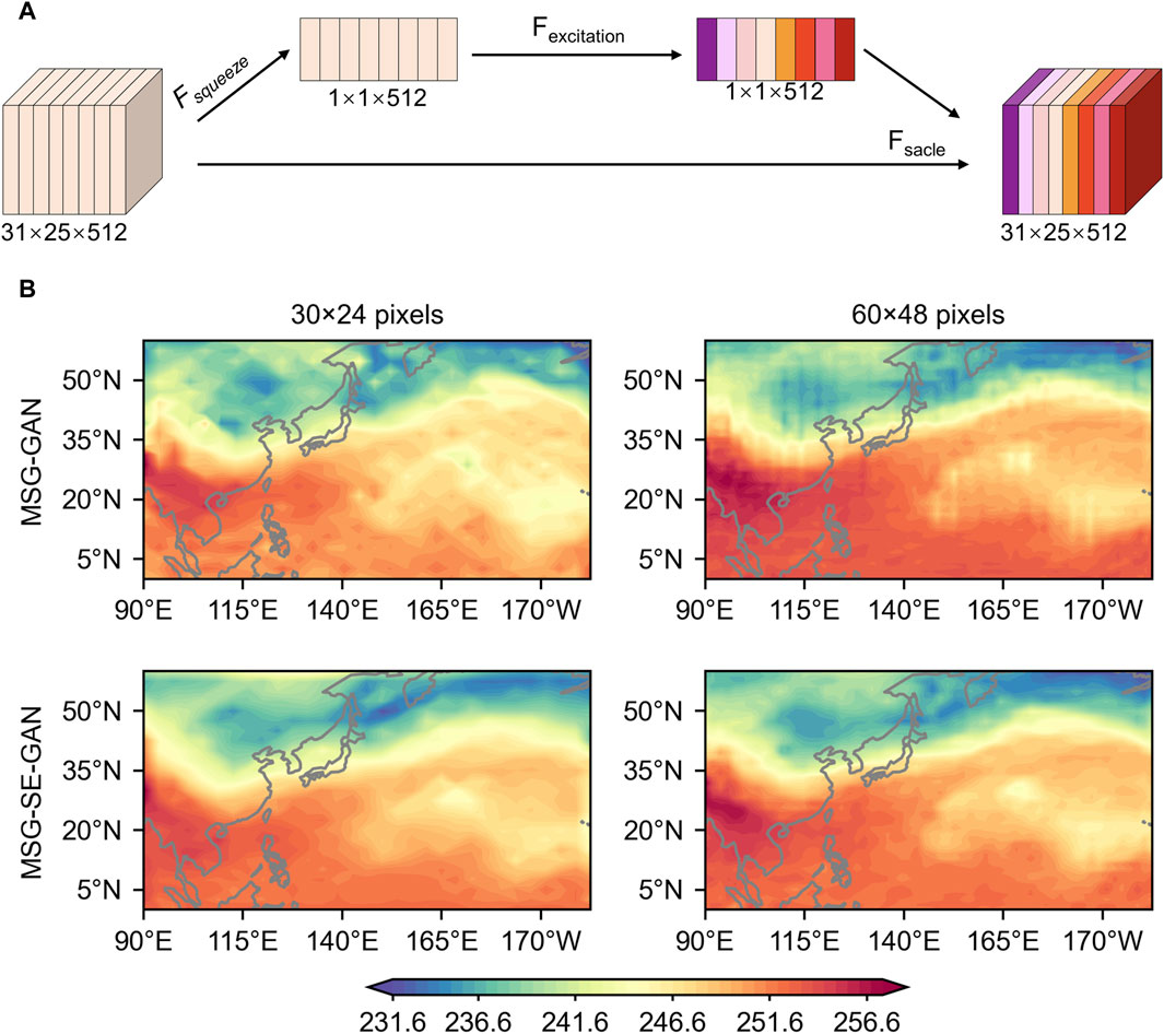
FIGURE 2. (A) SELayer schematic. Squeeze the 31×25 feature map to 1×1. Excitation predicts the importance of 512 channels with different colors representing the significance of each channel. Scale is a weighted process. (B) Ta variable with middle-size images of 31×25 and 60×48. The inclusion of the SELayer allows MSG-SE-GAN to better understand the underlying spatial structure and enhances the predictions.

The addition of the SELayer only slightly increases the model’s parameters but significantly improves the prediction accuracy. Taking the Ta variable as an example, Figure 2B depicts two middle-size images of Ta generated by MSG-GAN and MSG-SE-GAN on the validation set for comparison. It is obvious that, due to the difficulty of learning directly from 1-channel to 512-channel, the MSG-GAN cannot learn the underlying features of the image well. The MSG-SE-GAN, on the other hand, has substantially enhanced its performance in the mid-level resolutions and enhanced its understanding of underlying spatial structure of Ta. Therefore, the MSG-GAN is used as a baseline and participates in the validation and evaluation as a downscaling model along with the MSG-SE-GAN.

2.3 Training and validation settings

2.3.1 Training configuration

In our setting, the loss function for training MSG-GAN and MSG-SE-GAN is WGAN-GP (Wasserstein GAN with gradient penalty, Gulrajani et al., 2017). Training is a concept of adversarial learning, as it lies in the rivalry between two neural networks. In practice, we constrain the model through the WGAN-GP loss function, just like in a minimax game. For generator, G tries to minimize the Wasserstein distance between a real and a generated distribution. Conversely, for discriminators, D tries to maximize it to distinguish between ground truth and generated data. The WGAN-GP loss functions, as employed in this paper, take the form:

$L_D=E_{\stackrel{\sim }{x}\sim P_g}\left[D\left(\stackrel{\sim }{x}\right)\right]-E_{x\sim P_r}\left[D\left(x\right)\right]+\lambda E_{\widehat{x}\sim P_{\widehat{x}}}\left[{\left({‖{\nabla }_{\widehat{x}}D\left(\widehat{x}\right)‖}_2-1\right)}^2\right](1)$

$L_G=-E_{\stackrel{\sim }{x}\sim P_g}\left[D\left(\stackrel{\sim }{x}\right)\right](2)$

Where L_D and L_G are the loss functions for the discriminator and the generator, respectively, with a gradient penalty weight γ =10 (Gulrajani et al., 2017). P_r is the real data distribution and P_g is the generated distribution implicitly define by $\stackrel{\sim }{x}=G\left(z\right)$, where z is LR input taken in by the generator. The $\widehat{x}$ is randomly sampled from the real and generated data:

$\widehat{x}=\epsilon x+\left(1-\epsilon \right)\stackrel{\sim }{x},\epsilon \sim u\left(0,1\right)(3)$

Since the discriminator is a function of multiple input images generated by the generator, we modify the gradient penalty to be the average of the penalties over each input. Each convolution is followed by leaky rectified linear unit (LReLU) activation functions with α = 0.2 (Maas et al., 2013). The Adam optimizer (Kingma and Ba, 2014) is used for both the generator and the discriminator, with learning rates of 0.003 and 0.001. Training stabilization technologies such as Pixel Normalization (PixNorm) and Mini-batch Standard Deviations (MinBatchStdDev, Karras et al., 2019) are implemented within the model. PixNorm is embedded in the generator after each convolution to normalize the feature vectors. The MinibatchStdDev enhances the discriminator’s discriminative ability, allowing it to distinguish between real and generated samples more effectively. The model is trained with a batch size of 16 for 1,260 batches. The generator model weights are saved as checkpoints every 200 batches to facilitate model selection for validation purposes. Training a single model for a variable takes approximately 3 days on a single NVIDIA A100 GPU.

2.3.2 Assessment metric

This section describes the metrics used in this paper to validate the performance of the network.

• Peak to Signal Noise Ratio (PSNR)

$PSNR=10\bullet {\mathit{log}}_{10}\left(\frac{{\mathit{MAX}}^2}{MSE}\right)\left[dB\right](4)$

Where MAX is the maximum value in the image and MSE is the mean square error of the downscaling image. A higher PSNR value indicates lower distortion. It is a widely used objective image assessment metric based on the error between corresponding pixels.

• Structural Similarity Index Metric (SSIM)

$SSIM\left(X,Y\right)=\frac{\left(2{\mu }_x{\mu }_y+C_1\right)\bullet \left(2{\sigma }_{xy}+C_2\right)}{\left({\mu }_x^2+{\mu }_y^2+C_1\right)\bullet \left({\sigma }_x^2+{\sigma }_y^2+C_2\right)}(5)$

where X and Y represent the generated and the real sample, respectively. μ is the mean, σ is the covariance between X and Y, C₁, C₂, C₃ = 0.5×C₂, are constant values. SSIM is a metric for measuring the structural similarity between two images, yielding a value between 0 and 1 (Wang et al., 2004). Higher values indicate greater similarity between the two images. It calculates the difference between the images not only by considering corresponding pixels but also by taking into account the area of pixels around that position.

• Fréchet Inception Distance (FID)

$FID={‖{\mu }_r-{\mu }_g‖}^2+T_r\left(\sum r+\sum g-2{\left(\sum r\sum g\right)}^{\frac{1}{2}}\right)(6)$

Where μ_r and μ_g represents the feature means of real and generated images, respectively, while ∑r and ∑g denotes the covariance matrices of real and generated images. FID is a metric used to measure the distance between the distributions of real and generated images (Heusel et al., 2017). It quantifies the similarity between generated and real images by extracting feature vectors using a pre-trained Inception network (Simonyan and Zisserman, 2014) and then calculating the Fréchet distance between the two sets of feature vectors. FID is a commonly used metric in the field of GANs; a lower value indicates that the generated distribution is more similar to the real distribution.

2.3.3 Downscaling model selection

Figure 3 compares the stability of MSG-GAN and MSG-SE-GAN during training for the Ta variable on the validation set (results for the other variables are comparable). Both models exhibit rapid decreases or increases in all metrics during the early stages, and converge at approximately the 35th epoch, indicating that the mapping learning process is very rapid and efficient. The remaining training time is used to strengthen the model’s ability to perceive complex details, geometric structures, and high-frequency details. Though simultaneous training of the model at multiple scale layers slows the speed of each epoch, fewer epochs are required to achieve convergence. It is noteworthy that MSG-SE-GAN outperforms MSG-GAN across all metrics. Finally, we select an optimal model by referencing the synthesized PSNR×SSIM×FID^-1 score, determining whether the model’s metrics have converged, and manually inspecting checkpoint models on the validation set.

FIGURE 3

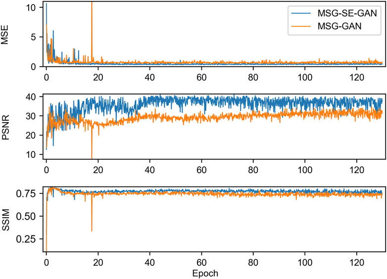
FIGURE 3. The variation of MSE, PSNR, and SSIM for the Ta variable highest resolution on the validation set as training iterations progress.

2.4 Tropical cyclone tracking algorithm

A Geophysical Fluid Dynamics Laboratory (GFDL) tropical cyclone tracking algorithm named TSTORMS was used to detect TCs in this paper (http://www.gfdl.noaa.gov/tstorms). The specific settings are as follows. (1) The local minimum in SLP is searched and located by fitting a biquadratic function to the SLP data. If a closed contour with a radius of 3,000 km contains both a minimum SLP and a maximum vorticity (greater than 1.6×10⁻⁴ s^-1), the center of the low is retained as a candidate cyclone. The maximum 10-m wind speed within the closed contours is considered to be the storm’s maximum wind speed at that time. (2) The warm core is computed as the mean atmospheric temperature between 500 and 250 hPa. The maximum mean atmospheric temperature must be at least 1 °C higher than the surrounding grid points, with its coordinates located within 1° of the low-pressure center. (3) At each 6-hourly time step, the storm center is linked to a trajectory by taking a low-pressure center at time T0 and considering the same cyclone at time T1 if the distance is less than 1,600 km. (4) A TC and resultant trajectories must satisfy the conditions mentioned above for at least 3 days, with at least 24 consecutive hours of warm core and maximum wind speeds exceeding 17 m s^-1.

3 Results

3.1 Model validation

After training the MSG-GAN and MSG-SE-GAN models for all variables, in this subsection, we include bilinear interpolation and SRCNN model for the inter-model comparison. Bilinear interpolation is widely adopted in climate research owing to its simplicity and computational efficiency. The SRCNN represents a deep learning model employed for the SR reconstruction of images. Dong et al. (2015) claimed that the model has the capability to effectively improve the resolution of an image while maintaining the clarity of the image details. The SRCNN is also often used to compare the results of the models (Shi et al., 2016; Kim et al., 2021).

Table 1 compares quantitatively the scores of assessment metrics for the Ta variable obtained by different downscaling models, including PSNR, SSIM, FID and PSNR×SSIM×FID^-1. Results for other meteorological variables are highly comparable. In general, a PSNR value in the range of 30–40 dB typically indicates good image quality (with noticeable but acceptable distortion), while values exceeding 40 dB suggest excellent image quality (close to the original image). The MSG-SE-GAN is the only model that surpasses 40 dB, well ahead of other models. The MSG-GAN also outperforms bilinear interpolation and the SRCNN model. The PSNR score is limited for it only considers the difference between the corresponding pixels. As a solution to this limitation, the SSIM score is utilized to quantify the structural similarity between two images. The highest SSIM score is still obtained by the MSG-SE-GAN, followed by the MSG-GAN. The FID score is widely used to evaluate generative models because of its consistency with human inspection and sensitivity to small changes in the real distribution. It is used to quantify the distribution disparity between the real and generated images. The FID score of MSG-SE-GAN is only slightly lower than that of the MSG-GAN model. Both the MSG-GAN and MSG-SE-GAN models significantly outperform other models, producing distributions that closely resemble the real data. It is noteworthy that all downscaling models based on deep learning outperform bilinear interpolation across all metrics. Furthermore, the MSG-SE-GAN model has the highest synthesized score of PSNR×SSIM×FID^-1.

TABLE 1

TABLE 1. Metric scores obtained by different models on validation set for Ta variable.

3.2 Power spectral density

A key indicator for describing the energy distribution of data at different spatial frequencies is power spectral density (PSD). Higher spatial frequencies reflect more rapid and localized changes, and higher power spectral density indicates greater energy at the corresponding spatial frequencies. Since the wind shows much higher spatial variations than Ta, the PSD analyses is conducted for the variable of 850 hPa wind $\left(\sqrt{{Ua}^2+{Va}^2}\right)$ and shown in Figure 4. The results for the near surface wind are highly similar (figure not shown).

FIGURE 4

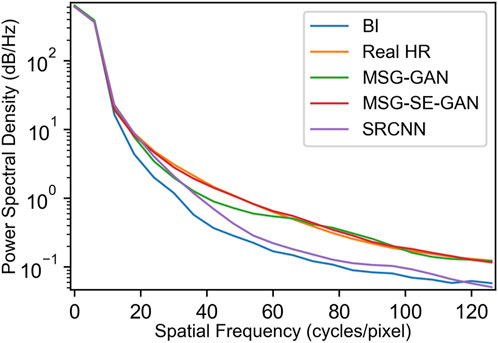
FIGURE 4. Power spectral density for 850 hPa wind on the validation set.

The MSG-GAN and the MSG-SE-GAN models are closer to the power spectral density of true data at higher frequencies, suggesting that both models have the ability to capture high-frequency information in the wind fields. However, bilinear interpolation and SRCNN fall off significantly at much finer scales. This is probably because the multi-scale technique learns the distribution of the data at each scale, but bilinear interpolation is unable to do so. While the SRCNN may perform better than bilinear interpolation, it still does not exhibit the capability to learn the distribution at various scales effectively. Interestingly, the MSG-GAN does not perform as well as the MSG-SE-GAN at lower frequencies; the PSD of MSG-GAN is significantly lower than that of MSG-SE-GAN and ground true data at spatial frequencies of 20–60 for the MSG-GAN lacks details at larger scales. In sum, the MSG-SE-GAN demonstrates superior capability in capturing underlying spatial structures and contains more information than MSG-GAN at larger scales, which can be attributed to the inclusion of the SENet model.

3.3 Examples of the downscaled fields for all variables

Since the MSG-GAN and MSG-SE-GAN are much better than bilinear interpolation and SRCNN in term of downscaling meteorological data, hereafter, the comparison is conducted mainly between the MSG-GAN and MSG-SE-GAN models for simplicity. We visualize the downscaled results of the MSG-GAN and MSG-SE-GAN models for TC-related variables, including sea level pressure, vertical mean temperature between 500 and 250 hPa, wind at 850 hPa, and near-surface wind, which allows for a more intuitive assessment of the models’ performance.

Here, we randomly select 2 TCs; one represents the weak TC and the other the strong TC (Figures 5, 6). The black box in Figures 5, 6 highlights the low-pressure center of the TCs. For the case of weak TC, it is evident that the TC intensity in the LR does not reach the level observed in the HR, and the location of the lowest pressure exhibits an east-northeastern offset (Figure 5A). However, in the downscaled results from MSG-GAN and MSG-SE-GAN, there is a significant enhancement of the TC’s intensity (Figures 5B–D). Particularly in the MSG-SE-GAN model, the position, structure, and, notably, intensity of the TC’s low-pressure center almost perfectly match the real HR (Figures 5B,D). The vertical mean temperature between 500 and 250 hPa at the same moment as the sea level pressure highlights the warm core structure of the TC. In the LR, there is no evident temperature maximum at the location of the TC center (Figure 5E), whereas both the real HR image and the downscaled HR images generated by the MSG-GAN and MSG-SE-GAN models exhibit the warm core structure of the TC with similar intensities. As for 850 hPa wind field and near-surface wind, we need to calculate the distance from the low-pressure center to the 850 hPa vorticity maximum in the TC detection process, and thus the 850 hPa wind field together with the vorticity field are shown in Figure 5I–L. There is a noticeable deviation of the vorticity maximum in the LR cyclonic structure from the HR ground truth (Figures 5G,I). The MSG-GAN model shows some improvement in capturing the cyclonic structure, with the vorticity maximum slightly westward of the HR ground truth (Figures 5G, K). However, the downscaled results from the MSG-SE-GAN model almost perfectly reproduce the cyclonic structure of the HR ground truth (Figures 5G, L). For the near-surface wind, the HR ground truth and the downscaled HR generated by the models are closer in terms of wind speed and structure. Particularly noteworthy is that both the location and amplitude of MSG-SE-GAN’s maximum TC wind speed are closer to the ground truth than those of MSG-GAN; the maximum wind speed of MSG-SE-GAN reaches the HR ground truth speed of over 20 m s^-1 (Figures 5N, P).

FIGURE 5

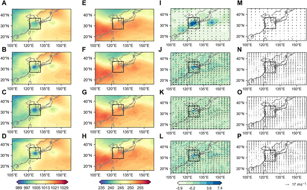
FIGURE 5. (A–D) SLP (units: hPa), (E–H) Ta (units: (C), (I–L) 850 hPa wind (vectors; units: m s^-1) and vorticity (shaded; units: 10^–4 s^-1) and (M–P) near-surface wind (vectors; units: m s^-1) generated by bilinear interpolation, MSG-GAN and MSG-SE-GAN models compared with their HR ground truth. The black box highlights the presence of a weak TC.

FIGURE 6

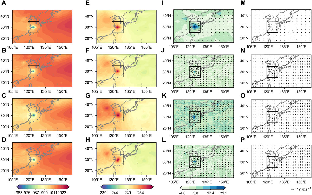
FIGURE 6. The same as in Figure 5, but with the presence of a strong TC.

Similarly, for the case of a strong TC, the MSG-SE-GAN also captures better the TC structure similated in the HR ground truth than other downscaling models (Figure 6), and we do not elaborate the detailed superiority for sake of conciseness. From an overall perspective, the models have produced downscaled results that are more detailed and visually realistic. The downscaled results of MSG-GAN and MSG-SE-GAN exhibit better consistency with the HR ground truth. In particular, the MSG-SE-GAN model demonstrates an advantage over the MSG-GAN model in preserving details and accuracy.

3.4 Application of HR TC tracking

The above results indicate that MSG-GAN and MSG-SE-GAN are effective in downscaling the TC-related variables, and their performance surpasses that of linear interpolation and the SRCNN model. Therefore, we apply the two models to downscale the outputs of HadGEM3-GC31-LM and compare the TC activities in the downscaling models to those directly simulated by the HadGEM3-GC31-HM to assess synthesized effects of the downscaling. We apply the TC tracking algorithm named TSTORMS to detect TCs as mentioned in section 2.4.

Figures 7A–D illustrates the climatological TC track density in the WNP based on outputs of HadGEM3-GC31-LM, MSG-GAN, MSG-SE-GAN and HadGEM3-GC31-HM by the same TC detection algorithm TSTORMS. It is apparent that even after applying bilinear interpolation to downscale HadGEM3-GC31-LM to HR data, the TC track density in the LR GCM is significantly lower than those in its HR version (Figures 7A, B). In contrast, the downscaled results from both the MSG-GAN and MSG-SE-GAN models substantially increase the number of TC (Figures 7B, D). Particularly, the climatological TC track density in the MSG-SE-GAN model closely resembles that of HadGEM3-GC31-HM, the MSG-SE-GAN shows the highest pattern correlation coefficient (PCC) of 0.88 and the lowest the root mean square error (RMSE) of 4.87.

FIGURE 7

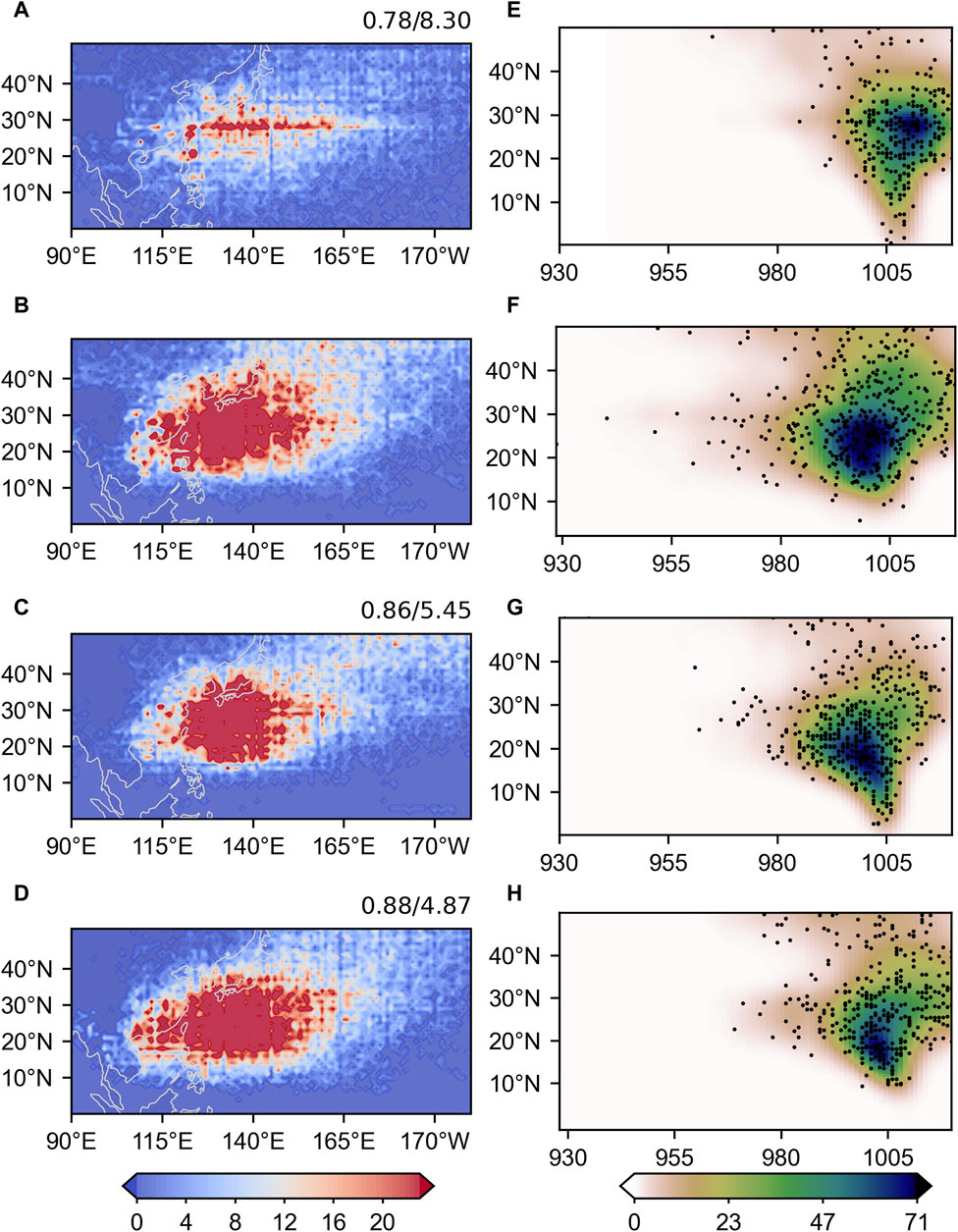
FIGURE 7. Climatological TC track density (1°×1°) and the Joint PDF of the TC MSLP and its latitudes generated by (C, G) MSG-GAN and (D, H) MSG-SE-GAN models, compared with that of (A, E) HadGEM3-GC31-LM (bilinear interpolated) and (B, F) HadGEM3-GC31-HM model data in the western North Pacific during July-October from 1980 to 2014. The upper right values represent the PCCs and RMSEs between each model and HadGEM3-GC31-HM (A, C, D). In the Joint PDF, TC density is shaded (units: number of TC per grid), with each dot representing a TC.

To investigate the TC intensity, the joint probability density function (PDF) of the TC minimum sea level pressure (MSLP) and the latitude where the TCs achieve the MSLP is also presented in Figures 7E–H. The joint PDF based on the HadGEM3-GC31-HM suggests that the most of TCs peak around 20°N (Figure 7F). However, the HadGEM3-GC31-LM differs dramatically from its HR version by simulating generally weaker TCs, fewer cases of strong TCs, higher mean peaking latitude, and more cases of TCs peaking near the equator (Figures 7E,F). After applying the MSG-GAN, the PDF becomes closer to the HadGEM3-GC31-HM by increasing the cases of strong TCs between 20˚-30˚N (Figures 7F,G). The MSG-SE-GAN model proposed in this study produce the most similar PDF to that of HadGEM3-GC31-HM by further reducing the cases of TCs peaking between 0 and 10˚N (Figures 7F,H).

Finally, we testy portability of our downscaling models to other independent LR GCMs. We have applied the MSG-GAN and MSG-SE-GAN models trained and tested by the HadGEM3-GC31 models to downscale the outputs of standard EC-Earth3P (100 km). Also, we compare the TC activities in the downscaling models to those directly simulated by the EC-Earth3P-HR (50 km) by using the same TC detection algorithm TSTORMS. As shown in Figures 8A,B, the climatological TC track density in the WNP in the standard EC-Earth3P is substantially lower than that in the EC-Earth3P-HR even after the bilinear interpolation. Both of the MSG-GAN and MSG-SE-GAN can substantially improve the TC track simulation, with the MSG-SE-GAN having the most similar track density as the EC-Earth3P-HR, with the highest PCCs of 0.74 and lowest RMSE of 4.8 (Figures 8B,D). Similarly, the joint PDF of the TC MSLP and its occurring latitudes are compared (Figures 8E–H). It is not surprising to find that the MSG-GAN simulates the PDF more similar to the EC-Earth3P-HR than the standard EC-Earth3P by increasing the TC intensity and reducing the number of TC peaking at high latitudes (Figures 8F,G). Also, the PDF of MSG-SE-GAN shows the closest pattern to that of the EC-Earth3P-HR by further reducing the cases of TC peaking between 0 and 10˚N (Figures 8F,H). The above analysis indicates that the MSG-SE-GAN shows the highest skills in downscaling the LR GCMs and has the portability among the LR GCMs.

FIGURE 8

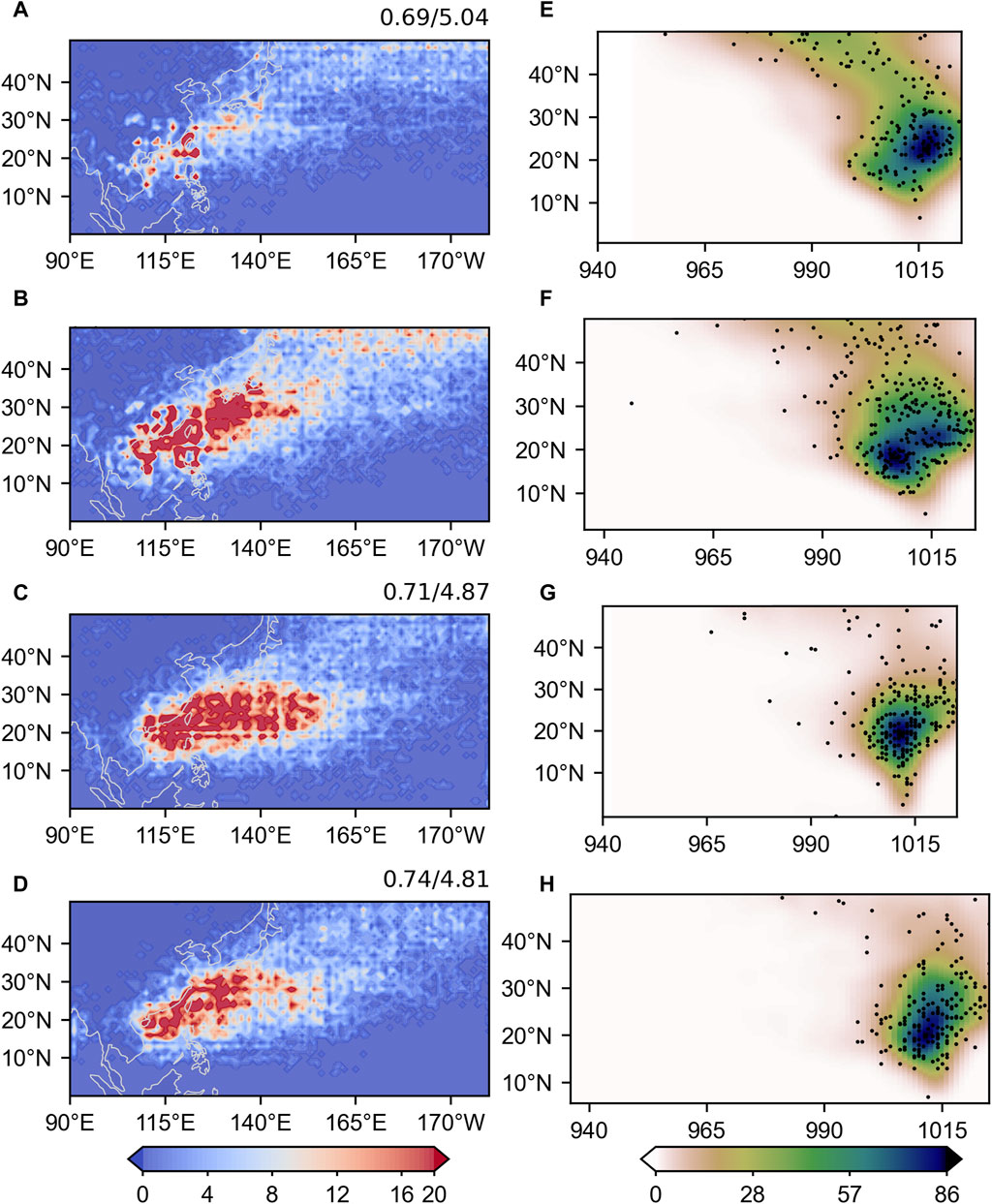
FIGURE 8. Climatological TC track density (1°×1°) and the Joint PDF of the TC MSLP and its latitudes generated by (C, G) MSG-GAN and (D, H) MSG-SE-GAN models, compared with that of (A, E) standard EC-Earth3P (bilinear interpolated) and (B, F) EC-Earth3P-HR model data in the western North Pacific during July-October from 1980 to 2014. The upper right values represent the PCCs and RMSEs between each model and EC-Earth3P-HR (A, D). In the Joint PDF, TC density is shaded (units: number of TC per grid), with each dot representing a TC.

4 Conclusion and discussion

In this study, we have adapted the MSG-GAN model for downscaling meteorological variables and further improved it to the MSG-SE-GAN model by incorporating the SELayer. Both models are capable of downscaling the input LR data by a factor of 10. We selected the HR version of HadGEM3-GC31 model to train and test our downscaling models. The results demonstrate that compared to the MSG-GAN, the MSG-SE-GAN can capture the underlying spatial structure more accurately. It also shows faster convergence as reflected by the maximum resolution MSE, PSNR, and SSIM metrics on the validation dataset, which signifies its efficacy in the learning process. Quantitative assessments using metrics including PSNR, SSIM, FID and the synthesized PSNR×SSIM×FID^-1 confirm the superiority of MSG-SE-GAN over bilinear interpolation, the SRCNN and the MSG-GAN. Power spectral analysis clearly reveals the inclusion of the SELayer in the MSG-SE-GAN model leads to better capture of underlying spatial structures than the MSG-GAN. Moreover, through visualization, we observed that the MSG-SE-GAN demonstrate an advantage in preserving details and accuracy of TC-related variables.

Based on the success of MSG-SE-GAN on downscaling the LR data that are coarsely interpolated from the HadGEM3-GC31-HM, we utilize the MSG-SE-GAN to downscale the real outputs of HadGEM3-GC31-LM and compare the TC activities in the MSG-SE-GAN to those in the HadGEM3-GC31-HM and the MSG-GAN model. The MSG-SE-GAN simulates most similar patterns of TC track density and joint PDF of TC peaking intensity and latitude with the HadGEM3-GC31-HM. In addition, we apply the MSG-SE-GAN to downscale the outputs of another independent LR GCM, the standard EC-Earth3P. It also simulates very similar TC activities with the corresponding HR GCM, the EC-Earth3P-HR. This suggests possible utility of MSG-SE-GAN to downscale a broad range of LR GCMs.

In this study, we aim to develop a deep learning-based statistical model to downscale the LR GCMs to mimic the performance of their corresponding HR GCMs rather than the observations. In this regard, the MSG-SE-GAN serves as a pseudo HR GCM that can increase the resolution of LR GCM outputs as if the resolutions of the LR GCMs themselves are increased. This is particularly important for the study of local extreme events under global warming because most CMIP6 models only provide the LR climate change projections. Here, the inputs of the model in this study are single variables, and our emphasis is on learning the mapping relationship between LR and HR to pursue univariate downscaling accuracy as much as possible. Since these variables, such as the zonal wind, meridional wind and air temperature, are physically constrained by Navier-Stokes equations in the GCMs, it would be better to further develop our model in our future study to enable the inputs of multiple variables and simultaneously downscale them, by which the physical constraint among the variables can be retained to some extent. In addition, we only use HadGEM3-GC31-HM outputs to train the downscaling model here. Considering the PRIMAVERA project has six pairs of HR and LR GCMs, we will include the outputs of different GCMs to train the model to improve the model portability. Based on the improved MSG-SE-GAN, we will downscale the LR climate change simulation and explore possible consensus among the CMIP6 models on the TC changes under different warming scenarios.

Data availability statement

The original contributions presented in the study are included in the article/Supplementary material, further inquiries can be directed to the corresponding author.

Author contributions

AC: Writing–original draft. CY: Writing–review and editing.

Funding

The author(s) declare financial support was received for the research, authorship, and/or publication of this article. This study is financially supported by the National Natural Science Foundation of China (42088101).

Acknowledgments

The analyses were conducted in the supercomputer in the High Performance Computing Center of Nanjing University of Information Science and Technology. The authors would like to thank the CMIP6 modelling groups for providing data (https://esgf-node.llnl.gov/projects/cmip6/).

Conflict of interest

The authors declare that the research was conducted in the absence of any commercial or financial relationships that could be construed as a potential conflict of interest.

Publisher’s note

All claims expressed in this article are solely those of the authors and do not necessarily represent those of their affiliated organizations, or those of the publisher, the editors and the reviewers. Any product that may be evaluated in this article, or claim that may be made by its manufacturer, is not guaranteed or endorsed by the publisher.

References

Anandhi, A., Srinivas, V. V., Kumar, D. N., and Nanjundiah, R. S. (2009). Role of predictors in downscaling surface temperature to river basin in India for IPCC SRES scenarios using support vector machine. Int. J. Climatol. A J. R. Meteorological Soc. 29 (4), 583–603. doi:10.1002/joc.1719

CrossRef Full Text | Google Scholar

Baño-Medina, J., Manzanas, R., and Gutiérrez, J. M. (2020). Configuration and intercomparison of deep learning neural models for statistical downscaling. Geosci. Model Dev. 13 (4), 2109–2124. doi:10.5194/gmd-13-2109-2020

CrossRef Full Text | Google Scholar

Benestad, R. E., Chen, D., Mezghani, A., Fan, L., and Parding, K. (2015). On using principal components to represent stations in empirical–statistical downscaling. Tellus A Dyn. Meteorology Oceanogr. 67 (1), 28326. doi:10.3402/tellusa.v67.28326

CrossRef Full Text | Google Scholar

Chen, S. T., Yu, P. S., and Tang, Y. H. (2010). Statistical downscaling of daily precipitation using support vector machines and multivariate analysis. J. hydrology 385 (1-4), 13–22. doi:10.1016/j.jhydrol.2010.01.021

CrossRef Full Text | Google Scholar

Chen, X., Xu, C., Yang, X., Song, L., and Tao, D. (2018). Gated-gan: adversarial gated networks for multi-collection style transfer. IEEE Trans. Image Process. 28 (2), 546–560. doi:10.1109/TIP.2018.2869695

PubMed Abstract | CrossRef Full Text | Google Scholar

Clark, P. (2006). High resolution model progress and plans. Science Advisory Committee Paper, (11.9).

Google Scholar

Demory, M. E., Vidale, P. L., Roberts, M. J., Berrisford, P., Strachan, J., Schiemann, R., et al. (2014). The role of horizontal resolution in simulating drivers of the global hydrological cycle. Clim. Dyn. 42, 2201–2225. doi:10.1007/s00382-013-1924-4

CrossRef Full Text | Google Scholar

Doi, T., Vecchi, G. A., Rosati, A. J., and Delworth, T. L. (2012). Biases in the Atlantic ITCZ in seasonal–interannual variations for a coarse-and a high-resolution coupled climate model. J. Clim. 25 (16), 5494–5511. doi:10.1175/JCLI-D-11-00360.1

CrossRef Full Text | Google Scholar

Dong, C., Loy, C. C., He, K., and Tang, X. (2015). Image super-resolution using deep convolutional networks. IEEE Trans. pattern analysis Mach. Intell. 38 (2), 295–307. doi:10.1109/TPAMI.2015.2439281

PubMed Abstract | CrossRef Full Text | Google Scholar

Emanuel, K. A. (2013). Downscaling CMIP5 climate models shows increased tropical cyclone activity over the 21st century. Proc. Natl. Acad. Sci. 110 (30), 12219–12224. doi:10.1073/pnas.1301293110

PubMed Abstract | CrossRef Full Text | Google Scholar

Erlandsen, H. B., Parding, K. M., Benestad, R., Mezghani, A., and Pontoppidan, M. (2020). A hybrid downscaling approach for future temperature and precipitation change. J. Appl. Meteorology Climatol. 59 (11), 1793–1807. doi:10.1175/JAMC-D-20-0013.1

CrossRef Full Text | Google Scholar

Estrada, F., Guerrero, V. M., Gay-García, C., and Martínez-López, B. (2013). A cautionary note on automated statistical downscaling methods for climate change. Clim. change 120, 263–276. doi:10.1007/s10584-013-0791-7

CrossRef Full Text | Google Scholar

Eyring, V., Bony, S., Meehl, G. A., Senior, C. A., Stevens, B., Stouffer, R. J., et al. (2016). Overview of the coupled model intercomparison project Phase 6 (CMIP6) experimental design and organization. Geosci. Model Dev. 9 (5), 1937–1958. doi:10.5194/gmd-9-1937-2016

CrossRef Full Text | Google Scholar

Giorgi, F., Jones, C., and Asrar, G. R. (2009). Addressing climate information needs at the regional level: the CORDEX framework. World Meteorol. Organ. (WMO) Bull. 58 (3), 175.

Google Scholar

Glahn, H. R., and Lowry, D. A. (1972). The use of model output statistics (MOS) in objective weather forecasting. J. Appl. Meteorology Climatol. 11 (8), 1203–1211. doi:10.1175/1520-0450(1972)011<1203:TUOMOS>2.0.CO;2

CrossRef Full Text | Google Scholar

Gulrajani, I., Ahmed, F., Arjovsky, M., Dumoulin, V., and Courville, A. C. (2017). “Improved training of wasserstein gans,” in Advances in neural information processing systems, 30.

Google Scholar

Guo, M. H., Xu, T. X., Liu, J. J., Liu, Z. N., Jiang, P. T., Mu, T. J., et al. (2022). Attention mechanisms in computer vision: a survey. Comput. Vis. media 8 (3), 331–368. doi:10.1007/s41095-022-0271-y

CrossRef Full Text | Google Scholar

Haarsma, R., Acosta, M., Bakhshi, R., Bretonnière, P. A., Caron, L. P., Castrillo, M., et al. (2020). HighResMIP versions of EC-Earth: EC-Earth3P and EC-Earth3P-HR–description, model computational performance and basic validation. Geosci. Model Dev. 13 (8), 3507–3527. doi:10.5194/gmd-13-3507-2020

CrossRef Full Text | Google Scholar

Haarsma, R. J., Roberts, M. J., Vidale, P. L., Senior, C. A., Bellucci, A., Bao, Q., et al. (2016). High resolution model intercomparison project (HighResMIP v1. 0) for CMIP6. Geosci. Model Dev. 9 (11), 4185–4208. doi:10.5194/gmd-9-4185-2016

CrossRef Full Text | Google Scholar

Harris, L., McRae, A. T., Chantry, M., Dueben, P. D., and Palmer, T. N. (2022). A generative deep learning approach to stochastic downscaling of precipitation forecasts. J. Adv. Model. Earth Syst. 14 (10), e2022MS003120. doi:10.1029/2022MS003120

PubMed Abstract | CrossRef Full Text | Google Scholar

Hashmi, M. Z., Shamseldin, A. Y., and Melville, B. W. (2009). Statistical downscaling of precipitation: state-of-the-art and application of bayesian multi-model approach for uncertainty assessment. Hydrology Earth Syst. Sci. Discuss. 6 (5), 6535–6579. doi:10.5194/hessd-6-6535-2009

CrossRef Full Text | Google Scholar

Heusel, M., Ramsauer, H., Unterthiner, T., Nessler, B., and Hochreiter, S. (2017). GANs trained by a two time-scale update rule converge to a local nash equilibrium. arXiv e-prints. doi:10.48550/arXiv.1706.08500

CrossRef Full Text | Google Scholar

Hu, J., Shen, L., and Sun, G. (2018). “Squeeze-and-excitation networks,” in Proc. Conf. Comput. Vis. Pattern Recognit., IEEE, 7132–7141. doi:10.48550/arXiv.1709.01507

CrossRef Full Text | Google Scholar

Karnewar, A., and Wang, O. (2020). “Msg-gan: multi-scale gradients for generative adversarial networks,” in Proceedings of the IEEE/CVF conference on computer vision and pattern recognition, Los Alamitos, CA (IEEE), 7799–7808.

CrossRef Full Text | Google Scholar

Karras, T., Aila, T., Laine, S., and Lehtinen, J. (2018). “Progressive growing of gans for improved quality, stability, and variation,” in International Conference on Learning Representations, Vancouver, Canada. Available at: https://iclr.cc/Conferences/2018.

Google Scholar

Karras, T., Laine, S., and Aila, T. (2019). “A style-based generator architecture for generative adversarial networks,” in Proceedings of the IEEE/CVF conference on computer vision and pattern recognition, CVPR, 4401–4410.

CrossRef Full Text | Google Scholar

Kim, J., Shin, M., Kim, D., Park, S., Kang, Y., Kim, J., et al. (2021). “Performance comparison of SRCNN, VDSR, and SRDenseNet deep learning models in embedded autonomous driving platforms,” in International Conference on Information Networking, Jeju Island, Korea (South), 56–58. doi:10.1109/ICOIN50884.2021.9333896

CrossRef Full Text | Google Scholar

Kingma, D. P., and Ba, J. (2014). Adam: a method for stochastic optimization. (arXiv e-prints). doi:10.48550/arXiv.1412.6980

CrossRef Full Text | Google Scholar

Klein, W. H. (1948). Winter precipitation as related to the 700–mb circulation. Bull. Am. Meteorological Soc. 29 (9), 439–453. doi:10.1175/1520-0477-29.9.1.439

CrossRef Full Text | Google Scholar

Knutson, T. R., Sirutis, J. J., Zhao, M., Tuleya, R. E., Bender, M., Vecchi, G. A., et al. (2015). Global projections of intense tropical cyclone activity for the late twenty-first century from dynamical downscaling of CMIP5/RCP4. 5 scenarios. J. Clim. 28 (18), 7203–7224. doi:10.1175/JCLI-D-15-0129.1

CrossRef Full Text | Google Scholar

Ledig, C., Theis, L., Huszár, F., Caballero, J., Cunningham, A., Acosta, A., et al. (2016). Photo-realistic single image super-resolution using a generative adversarial network. (arXiv e-prints). doi:10.48550/arXiv.1609.04802

CrossRef Full Text | Google Scholar

Liu, J., Yuan, C., and Luo, J. J. (2023). Impacts of model resolution on responses of western North Pacific tropical cyclones to ENSO in the HighResMIP-PRIMAVERA ensemble. Front. Earth Sci. 11, 1169885. doi:10.3389/feart.2023.1169885

CrossRef Full Text | Google Scholar

Maas, A. L., Hannun, A. Y., and Ng, A. Y. (2013). “Rectifier nonlinearities improve neural network acoustic models,” in Proceedings of the 30th International Conference on Machine Learning, Atlanta, USA28 (3), Available at: https://ai.stanford.edu/∼amaas/papers/relu_hybrid_icml2013_final.pdf

Google Scholar

Manabe, S., and Stouffer, R. J. (1993). Century-scale effects of increased atmospheric C02 on the ocean–atmosphere system. Nature 364 (6434), 215–218. doi:10.1038/364215a0

CrossRef Full Text | Google Scholar

Murakami, H., Vecchi, G. A., Underwood, S., Delworth, T. L., Wittenberg, A. T., Anderson, W. G., et al. (2015). Simulation and prediction of category 4 and 5 hurricanes in the high-resolution GFDL HiFLOR coupled climate model. J. Clim. 28 (23), 9058–9079. doi:10.1175/JCLI-D-15-0216.1

CrossRef Full Text | Google Scholar

Pan, B., Hsu, K., AghaKouchak, A., and Sorooshian, S. (2019). Improving precipitation estimation using convolutional neural network. Water Resour. Res. 55 (3), 2301–2321. doi:10.1029/2018WR024090

CrossRef Full Text | Google Scholar

Rathmann, N. M., Yang, S., and Kaas, E. (2014). Tropical cyclones in enhanced resolution CMIP5 experiments. Clim. Dyn. 42, 665–681. doi:10.1007/s00382-013-1818-5

CrossRef Full Text | Google Scholar

Roberts, M. J., Camp, J., Seddon, J., Vidale, P. L., Hodges, K., Vanniere, B., et al. (2020). Impact of model resolution on tropical cyclone simulation using the HighResMIP–PRIMAVERA multimodel ensemble. J. Clim. 33 (7), 2557–2583. doi:10.1175/JCLI-D-19-0639.1

CrossRef Full Text | Google Scholar

Shi, W., Caballero, J., Huszár, F., Totz, J., Aitken, A. P., Bishop, R., et al. (2016). Real-time single image and video super-resolution using an efficient sub-pixel convolutional neural network. In In Proceedings of the IEEE conference on computer vision and pattern recognition, Las Vegas, USA, CVPR, pp. 1874–1883.

CrossRef Full Text | Google Scholar

Simonyan, K., and Zisserman, A. (2014). Very deep convolutional networks for large-scale image recognition. (arXiv preprint). doi:10.48550/arXiv.1409.1556

CrossRef Full Text | Google Scholar

Song, K., Zhao, J., Zhan, R., Tao, L., and Chen, L. (2022). Confidence and uncertainty in simulating tropical cyclone long-term variability using the CMIP6-HighResMIP. J. Clim. 35 (19), 6431–6451. doi:10.1175/JCLI-D-21-0875.1

CrossRef Full Text | Google Scholar

Stengel, K., Glaws, A., Hettinger, D., and King, R. N. (2020). Adversarial super-resolution of climatological wind and solar data. Proc. Natl. Acad. Sci. 117 (29), 16805–16815. doi:10.1073/pnas.1918964117

PubMed Abstract | CrossRef Full Text | Google Scholar

Taylor, K. E., Stouffer, R. J., and Meehl, G. A. (2012). An overview of CMIP5 and the experiment design. Bull. Am. meteorological Soc. 93 (4), 485–498. doi:10.1175/BAMS-D-11-00094.1

CrossRef Full Text | Google Scholar

Tselioudis, G., Douvis, C., and Zerefos, C. (2012). Does dynamical downscaling introduce novel information in climate model simulations of precipitation change over a complex topography region? Int. J. Climatol. 32 (10), 1572–1578. doi:10.1002/joc.2360

CrossRef Full Text | Google Scholar

Vandal, T., Kodra, E., Ganguly, S., Michaelis, A., Nemani, R., and Ganguly, A. R. (2017). DeepSD: Generating high resolution climate change projections through single image super-resolution. (arXiv e-prints, doi:10.48550/arXiv.1703.03126

CrossRef Full Text | Google Scholar

Villarini, G., and Vecchi, G. A. (2012). Twenty-first-century projections of North Atlantic tropical storms from CMIP5 models. Nat. Clim. Change 2 (8), 604–607. doi:10.1038/nclimate1530

CrossRef Full Text | Google Scholar

Vu, M. T., Aribarg, T., Supratid, S., Raghavan, S. V., and Liong, S. Y. (2016). Statistical downscaling rainfall using artificial neural network: significantly wetter Bangkok? Theor. Appl. Climatol. 126, 453–467. doi:10.1007/s00704-015-1580-1

CrossRef Full Text | Google Scholar

Wang, C., Xu, C., Yao, X., and Tao, D. (2019). Evolutionary generative adversarial networks. IEEE Trans. Evol. Comput. 23 (6), 921–934. doi:10.1109/TEVC.2019.2895748

CrossRef Full Text | Google Scholar

Wang, F., Tian, D., Lowe, L., Kalin, L., and Lehrter, J. (2021). Deep learning for daily precipitation and temperature downscaling. Water Resour. Res. 57 (4), e2020WR029308. doi:10.1029/2020WR029308

CrossRef Full Text | Google Scholar

Wang, Z., Bovik, A. C., Sheikh, H. R., and Simoncelli, E. P. (2004). Image quality assessment: from error visibility to structural similarity. IEEE Trans. image Process. 13 (4), 600–612. doi:10.1109/TIP.2003.819861

PubMed Abstract | CrossRef Full Text | Google Scholar

Wengel, C., Lee, S. S., Stuecker, M. F., Timmermann, A., Chu, J. E., and Schloesser, F. (2021). Future high-resolution El niño/southern oscillation dynamics. Nat. Clim. Change 11 (9), 758–765. doi:10.1038/s41558-021-01132-4

CrossRef Full Text | Google Scholar

White, B. L., Singh, A., and Albert, A. (2019). Downscaling numerical weather models with gans. AGU Fall Meet. Abstr. 2019, GC43D–1357.

Google Scholar

Williams, K. D., Copsey, D., Blockley, E. W., Bodas-Salcedo, A., Calvert, D., Comer, R., et al. (2018). The Met Office global coupled model 3.0 and 3.1 (GC3. 0 and GC3. 1) configurations. J. Adv. Model. Earth Syst. 10, 357–380. doi:10.1002/2017MS001115

CrossRef Full Text | Google Scholar

Wu, C. C., Zhan, R., Lu, Y., and Wang, Y. (2012). Internal variability of the dynamically downscaled tropical cyclone activity over the western North Pacific by the IPRC regional atmospheric model. J. Clim. 25 (6), 2104–2122. doi:10.1175/JCLI-D-11-00143.1

CrossRef Full Text | Google Scholar

Zhang, W., Villarini, G., Scoccimarro, E., Roberts, M., Vidale, P. L., Vanniere, B., et al. (2021). Tropical cyclone precipitation in the HighResMIP atmosphere-only experiments of the PRIMAVERA Project. Clim. Dyn. 57, 253–273. doi:10.1007/s00382-021-05707-x

CrossRef Full Text | Google Scholar