 Wenbin Cai
 Zirui Sun1
- 1College of Petroleum Engineering, Xi’an Shiyou University, Xi’an, Shaanxi, China
- 2College of Computer Science, Xi’an Shiyou University, Xi’an, Shaanxi, China
At present, more than 90% of China’s oil production equipment comprises rod pump production systems. Indicator diagram analysis of the pumping unit is not only an effective method for monitoring the current working condition of a rod pump production system but also the main way to prevent, detect, and rectify various faults in the oil production process. However, the identification of the pumping unit indicator diagram mainly involves manual effort, and the identification accuracy depends on the experience of the monitoring personnel. Automatic and accurate identification and classification of the pumping unit indicator diagram using new computer technology has long been the research focus of studies for monitoring the pumping unit working condition. In this paper, the indicator diagram is briefly introduced, and the AlexNet model is presented to distinguish the indicator diagram of abnormal wells. The influence of the step size, convolution kernel size, and batch normalization (BN) layer on the accuracy of the model is analyzed. Finally, the AlexNet model is improved. The improved model reduces the calculation cost and parameters, accelerates the convergence, and improves the accuracy and speed of the calculation. In the experimental analysis of abnormal well diagnosis, the data are preprocessed via data deduplication, binary filling, random line distortion, random scaling and stretching, and random vertical horizontal displacement. In addition, the image is expanded by transforming several well indicator diagrams. Finally, data sets of 10 types of indicator diagrams are created for better adaptability and application in the analysis and classification of indicator diagrams, and the ideal application effect is achieved in actual working conditions. In summary, this technology not only improves the recognition accuracy but also saves manpower. Thus, it has good application prospects in the field of oil production.
Introduction
Rod pump production systems constitute the predominant equipment in crude oil exploitation. Owing to the specific nature of their structural characteristics and working environment, their failure rate is high. Therefore, it is crucial to understand the working state of the pumping unit as well as to analyze and rectify faults in a timely and accurate manner (Li et al., 2013a; Reges et al., 2015). The indicator diagram is a closed curve composed of the load-versus-displacement curves. In the working process of the rod pumping unit, the obtained indicator diagram can be used to qualitatively analyze the working condition of the pumping unit, adjust the working parameters in a timely manner, and detect and eliminate faults. However, in actual production, the recognition and classification of the indicator diagram mainly involves manual effort, and the recognition efficiency is low. Deep learning, a new area of machine learning with successful applications in computer vision, speech recognition, and other fields, provides a new idea for solving problems such as image classification (Zhang, 2000; Xu et al., 2007; Bezerra et al., 2010; Sun et al., 2012; Li et al., 2013b),. As the analysis of the indicator diagram can be regarded as a type of image classification, it is technically feasible and of great practical significance to study the application of convolutional neural networks (CNNs) to the automatic identification and classification of the indicator diagram (Luan et al., 2011; Li, 2015).
Diagnosis of abnormal wells based on AlexNet model
In recent years, the use of computer technology for the diagnosis of abnormal wells has attracted considerable research attention. For example, expert systems, support vector machines, and fuzzy theory are used in the diagnosis of abnormal wells (Krizhevsky et al., 2012; Krizhevsky, 2014). These methods involve artificial feature extraction, i.e., feature extraction using classification methods such as pattern classification. However, the extraction process is manual and hence suffers from information loss and extraction errors, which affect the performance of the subsequent classification algorithms. In deep learning, a large amount of historical data can be used to automatically extract and learn features, which compensates for the shortcomings of manual feature extraction. According to the characteristics of the indicator diagram, the CNN algorithm is an innovative and widely applicable tool for the diagnosis of abnormal wells.
Figure 1 shows the AlexNet network model. The network model for image recognition consists of four basic elements: convolution layer, pooling layer, fully connected layer, and activation function (Xu et al., 2020). The pooling layer generally follows the convolution layer, and the fully connected layer is located at the end of the network to output the final feature vector. The activation function determines whether the neurons are activated for transmitting information. The main function of the convolution layer is to extract the features of the input indicator diagram. The core idea of convolution involves the local receptive field and weight sharing convolution process. After the convolution layer extracts the features, the generated feature map is passed to the next layer. The main function of the pooling layer is to compress the feature map and eliminate the influence of the space conversion of the indicator map. The last layer of the CNN is generally the fully connected layer, whose function is to convert the feature map of the input indicator diagram extracted by the previous convolution layer and pooling layer into the feature vector output. Thus, the diagnosis of abnormal wells is completed.
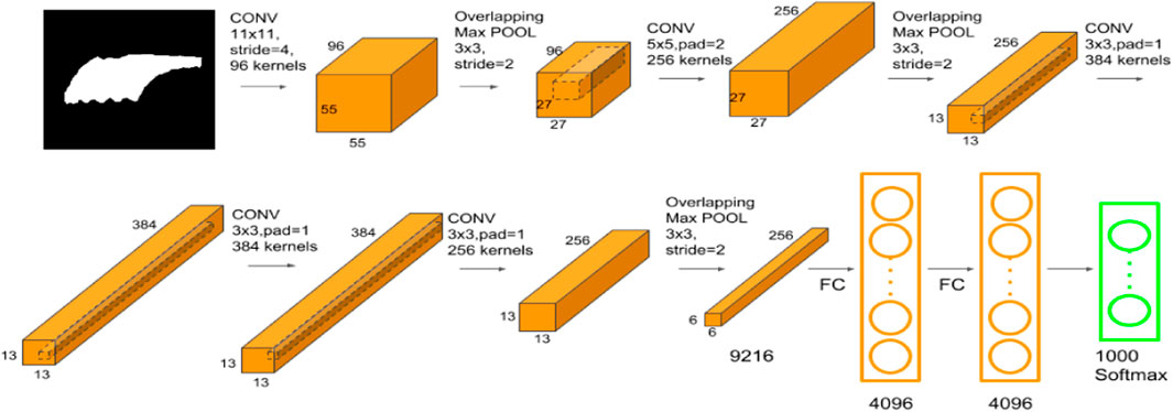
FIGURE 1. AlexNet network model.
The AlexNet experiment involves 80 iterations. The model is saved once every 10 iterations, and the accuracy, number of iterations, and loss error of the model are recorded. The accuracy of the network model is gradually stable after more than 20 iterations, and the recognition accuracy of the model test set is 97.3%, as shown in Figure 2A. Similarly, after around 20 iterations, the loss value gradually becomes stable and reaches convergence; the loss of the test set is around 0.02, as shown in Figure 2B. As can be seen from the confusion matrix shown in Figure 2C, the diagnostic accuracy of the AlexNet model for abnormal wells is relatively high. According to the diagnosis, error-prone situations that occur include fixed valve leakage, insufficient liquid supply and gas influence, and slow closing of the moving valve. However, the test set comprising nearly 1700 data includes less than 40 error data. Thus, the AlexNet network achieves high accuracy in indicator diagram classification for abnormal well diagnosis. Finally, the evaluation indexes of the model are as follows: accuracy rate, 96.58%; precision rate, 97.18%; recall rate, 95.97%; and F1 score, 96.22%.
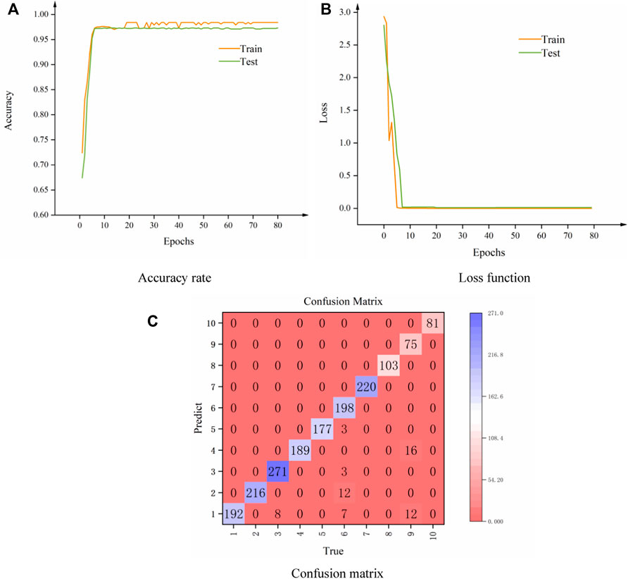
FIGURE 2. AlexNet training process. (A) Accuracy rate (B) Loss function (C) Confusion matrix.
Improvement of AlexNet model
Owing to the high memory consumption and low accuracy of the AlexNet model, the model is improved accordingly. The influence of various parameters on the diagnosis accuracy of abnormal wells is studied in detail. The model is optimized in terms of the convolution kernel size, batch normalization (BN) layer, and step length, and the parameters suitable for the diagnosis model of abnormal wells are selected. The early stopping method and dropout layer are used to prevent overfitting of the model. The number of iterations/epochs is set to 80, and the accuracy and error of the training and test sets are recorded once per epoch.
Influence of convolution kernel size on network model
1) 5*5 convolution kernel
The network model converges after around 20 iterations, and the loss converges to 0.08 for the test set. Figure 3 shows the good fitting performance of the network model.
2) 3*3 convolution kernel
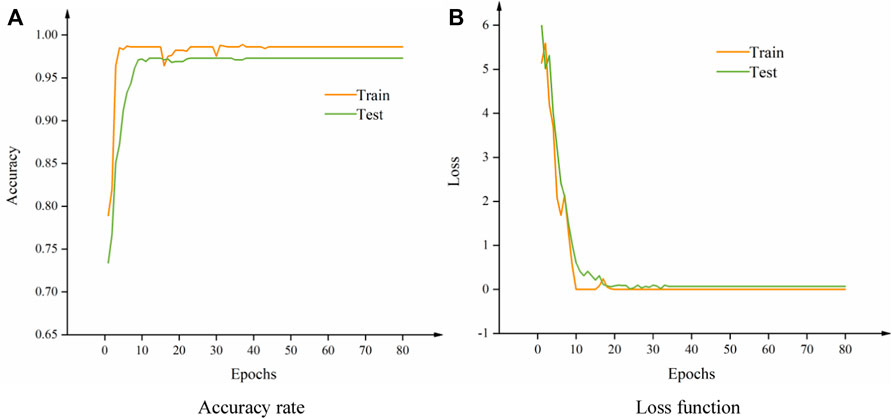
FIGURE 3. 5*5 Convolutional training process. (A) Accuracy rate (B) Loss function.
The network model converges after around 20 iterations, and the deviation is small. The 3*3 convolution kernel achieves better performance than the 5*5 convolution kernel, as shown in Figure 4. Hence, the 3*3 convolution kernel is a better choice。
3) 2*2 convolution kernel
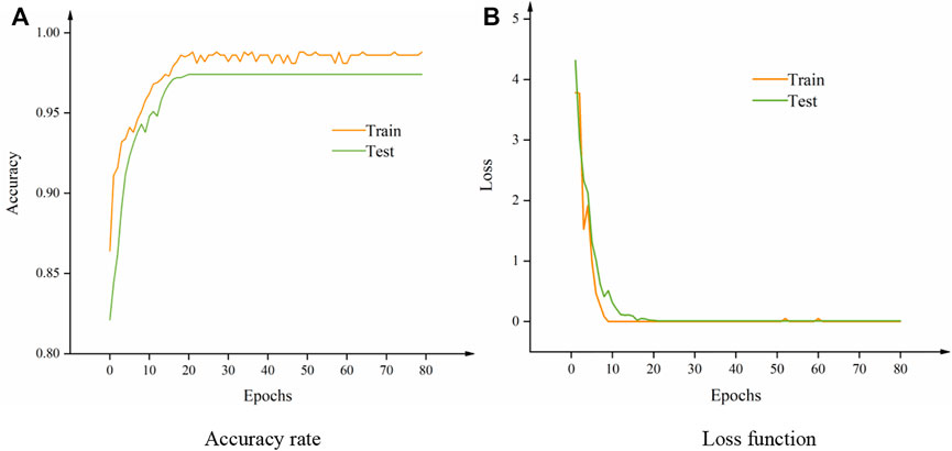
FIGURE 4. 3*3 Convolutional training process. (A) Accuracy rate (B) Loss function.
There is a certain gap between the 2*2 and 3*3 convolution kernels in terms of the fitting and accuracy, as shown in Figure 5. Hence, the usage rate of the 2*2 convolution kernel is low in common network models.
4) Comparative analysis of experiments
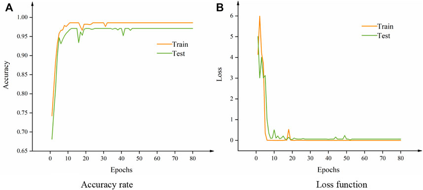
FIGURE 5. 2*2 convolution training process. (A) Accuracy rate (B) Loss function.
The size of the convolution kernel influences the performance of the network model. From the aforementioned experiments, the 3*3 convolution kernel is selected because it has the highest accuracy, relatively small number of parameters, and moderate memory consumption. Table 1 compares the performances of the three convolution kernel sizes.
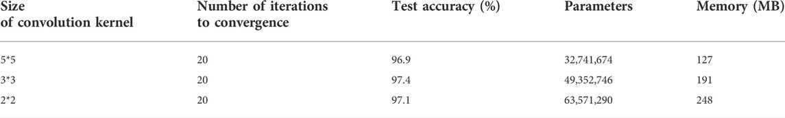
TABLE 1. Performance comparison of three convolution kernel sizes.
Influence of step size on network model
As can be seen from Table 2, the 2cs2 _ 3cs1 model outperforms the AlexNet model in terms of the accuracy, number of parameters, and memory consumption.
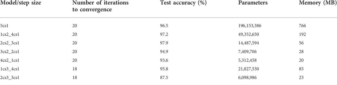
TABLE 2. Influence of step size on network performance.
Influence of BN layer on network model
In the training and testing processes of the network model, any change in the network input will affect the accuracy of the model. In particular, in the case of the deep network model, the number of iterations until convergence will increase (Huang, 2007; Yang, 2011). In the training process, if the distribution of the input in the previous layer changes significantly, the model will suffer from poor adaptability, which leads to difficulty in adjusting the parameters. Using the BN layer can reduce the dependence on data initialization and prevent problems caused by it (Chen et al., 2014; Yuan and Hu, 2015; Xu et al., 2019).
The experiment uses the AlexNet network model to add the BN layer in order to test the influence of the BN layer on the abnormal well diagnosis model. The number of iterations is 80, the initial learning rate is 0.01, and the batch size is 16.
Figures 6A,B show the accuracy curves of the abnormal well diagnosis model before and after adding the BN layer for the training and test sets, respectively. Figures 7A,B show the loss value curves of the abnormal well diagnosis model before and after adding the BN layer for the training and test sets, respectively. As can be seen from the curve of the training set, the loss value of the model with the BN layer decreases faster as the number of iterations increases, and the loss value is minimized when the number of iterations is around 10. Thus, adding the BN layer accelerates the convergence of the network model and makes it easier to extract the characteristics of image information. For the test set, the loss value of the model changes relatively smoothly. In general, the loss value of the model with the BN layer decreases faster than that of the model without BN layer. As can be seen from the accuracy change diagram, the model with the BN layer can achieve the highest accuracy faster, which can effectively reduce the training time to a certain extent.
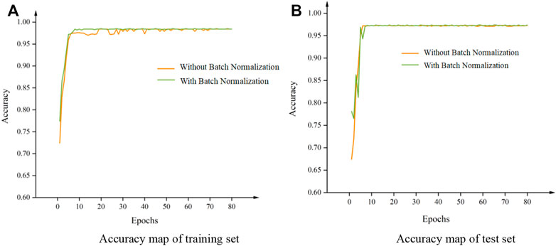
FIGURE 6. Comparison of step accuracy. (A) Accuracy map of training set (B) Accuracy map of test set.
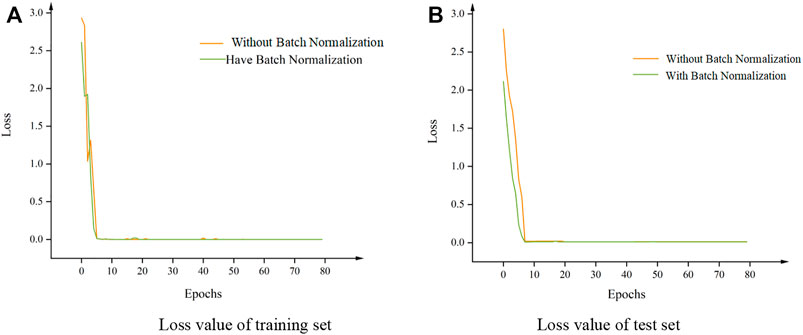
FIGURE 7. Comparison of step loss rate. (A) Loss value of training set (B) Loss value of test set.
Abnormal well diagnosis model based on improved AlexNet
The improved AlexNet model uses the 3*3 convolution kernel instead of the 11*11 or 5*5 convolution kernel, which reduces the calculation cost and number of parameters and accelerates the convergence. Figure 8 shows a schematic of the improved AlexNet network model.
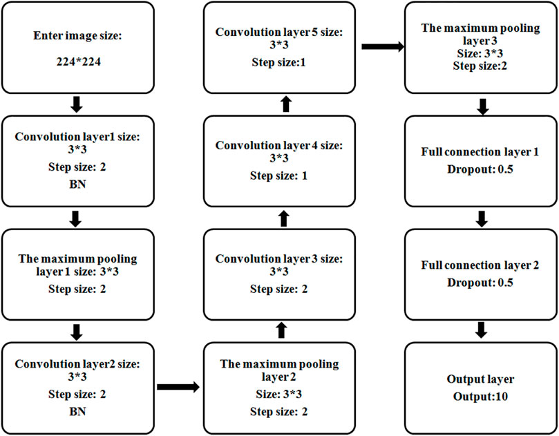
FIGURE 8. Improved AlexNet network model. In this study, VGG, LeNet, and other models are used for comparison.
The experimental results of the two models on the test set data are summarized in Table 3. The number of parameters and memory size of the AlexNet model are 57 million and 230 MB, respectively. The minimum memory consumption of the improved AlexNet is 56 MB. Compared with AlexNet, the number of parameters is reduced by more than 43 million and the memory consumption is reduced by 174 MB. Finally, the diagnostic classification accuracy of abnormal wells using the two models on the test set is listed in the table. As can be seen, the accuracy of the improved AlexNet is 97.9%.
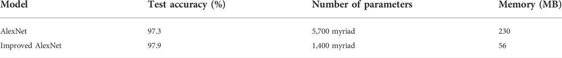
TABLE 3. Comparison of two models.
Experimental analysis of deep learning model
Experimental data preparation
In deep learning, owing to the small number of samples of training data, under-fitting will occur while training the network model (Wen et al., 2016; Zhang et al., 2016; Lu and Goodson, 2017; Xu et al., 2018). Therefore, an image expansion method based on the characteristics of the indicator diagram is proposed. Table 4 summarizes the transformation of the indicator diagram.
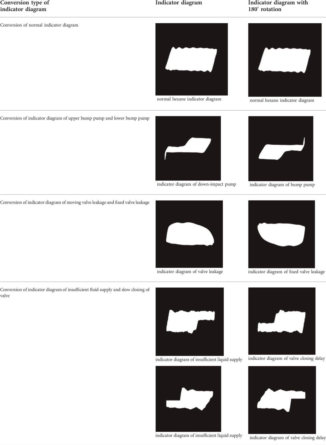
TABLE 4. Transformation of indicator diagram.
For an actual oil well, the abnormal indicator diagram data are less whereas the normal indicator diagram data are more. To ensure the generalization ability of the model and the balance of data, the normal indicator diagram is randomly deleted.
Creation of data sets
In this study, 10 types of indicator diagrams are collected, and 10 folders are created accordingly, as shown in Table 5. The indicator diagram data in Table 5 from Shengli Oilfield in China, there have been tens of thousands of rod pumping wells. Due to serious sand production, high water cut, strong corrosion, high viscosity of crude oil, insufficient liquid supply and other reasons, downhole accidents such as rod breaking, pump leakage and sand sticking often occur.
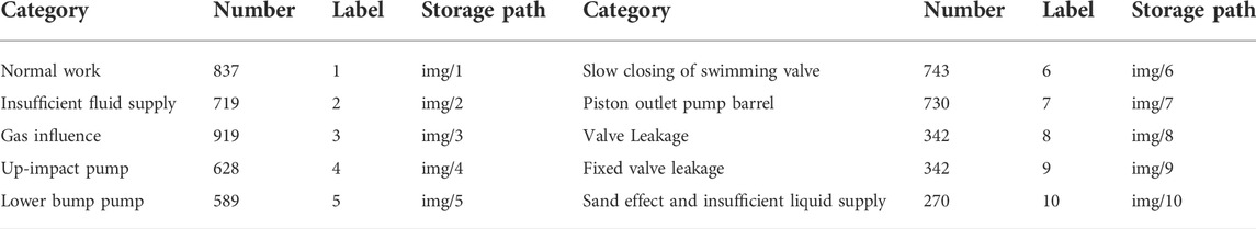
TABLE 5. Classification of indicator diagram.
Each indicator diagram is saved in a .txt file and named with a picture path tag, such as img/1/a001.jpg 1, for the model to read. After storage, the sequence is randomly disrupted; 70% is randomly selected as the training set and the remaining 30% is employed as the test set by using the method of leaving the set.
Application of improved AlexNet model to indicator diagram analysis
The trained CNN is used to analyze and diagnose the indicator diagram of the pumping unit, which is input to the improved AlexNet network model to judge the working condition type. The judgment results are shown in Table 6:
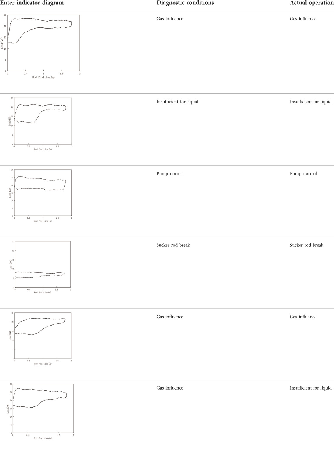
TABLE 6. Diagnostic results of indicator diagram.
As can be seen from the table, the accuracy of the improved model in the judgment of the working condition is 83.3%, which is basically consistent with the actual working condition, indicating that the improved model has good application prospects in actual working condition analysis.
Conclusion
In this study, an improved AlexNet model with a total of five convolution layers and a 3*3 convolution kernel was employed. In the first two convolution layers, the step size was 2, and in the last three convolution layers, the step size was 1. The pooling layer used was the maximum pooling layer, and the step size was 2. The BN layer was added behind convolution layers 1 and 2. Moreover, the memory consumption of the improved AlexNet model was reduced considerably, which accelerated the convergence and resulted in high accuracy in the analysis of actual working conditions. Finally, a comparison of the model parameters and calculation cost showed that the performance of the improved AlexNet model is superior. (Duan et al., 2018).
Data availability statement
The raw data supporting the conclusion of this article will be made available by the authors, without undue reservation.
Author contributions
Conceptualization, WC; methodology, ZS; validation, ZW; formal analysis, XW; investigation, YW; resources, GY; data curation, SP.
Funding
This work is supported by the National Natural Science Foundation of China (Grant No. 52074225). Xi’an petroleum university undergraduate innovation and entrepreneurship training program (Grant No. 202110705021).
Acknowledgments
The authors would like to thank all the reviewers who participated in the review, as well as MJEditor (www.mjeditor.com) for providing English editing services during the preparation of this manuscript.
Conflict of interest
The authors declare that the research was conducted in the absence of any commercial or financial relationships that could be construed as a potential conflict of interest.
Publisher’s note
All claims expressed in this article are solely those of the authors and do not necessarily represent those of their affiliated organizations, or those of the publisher, the editors and the reviewers. Any product that may be evaluated in this article, or claim that may be made by its manufacturer, is not guaranteed or endorsed by the publisher.
References
Yang, Y. (2011). And fault diagnosis system for rod pump wells based on pump power diagram analysis. Dailan: Dalian University of Technology.
Bezerra, M. A. D., Schnitman, L., Filho, M. D. A. B., and de Souza, J. A. M. F. (2010). “Pattern recognition for downhole dynamometer card in oil rod pump system using artificial neural networks,” in ICEIS2009—Proceedings of the 11th International Conference on Enterprise Information Systems,Volume AIDSS, Milan,Italy, May 6-10,2009 (DBLP), 351–355.
Chen, Y., Li, H., and Ji, Y. (2014). Expert system for downhole fault diagnosis of pumping unit based on neural network. Electron. Des. Eng. 22 (01), 130–132. doi:10.14022/j.cnki.dzsjgc.2014.01.006
Duan, Y., Yu, L., Sun, Q., and Xu, D. (2018). Improved Alexnet model and its application in well indicator diagram classification. Comput. Appl. Softw. 35 (07), 226–230+272. doi:10.3969/j.issn.1000-386x.2018.07.041
Huang, X. (2007). Research on intelligent integrated system for fault diagnosis of pumping wells. J. Petroleum Nat. Gas 29 (3), 156–158.
Krizhevsky, A. One weird trick for parallelizing convolutional neural networks[DB] ar Xiv preprint ar Xiv: 1404 5997, 2014
Krizhevsky, A., Sutskever, I., and Hinton, G. E. (2012). Imagenet classification with deep convolutional neural networks. Adv. neural Inf. Process. Syst., 25, 1097–1105. doi:10.1145/3065386
Li, K., Gao, X., Tian, Z., and Qiu, Z. (2013). Using the curve moment and the PSO-SVM method to diagnose downhole conditions of asucker rod pumping unit. Petroleum Sci. 10 (1), 73–80. doi:10.1007/s12182-013-0252-y
Li, K., Gao, X., Yang, W., Dai, Y-L., and Tian, Z. (2013). Multiple fault diagnosis of down-hole conditions of sucker-rod pumping wells based on Freeman chain code and DCA. Petroleum Sci. 10 (3), 347–360. doi:10.1007/s12182-013-0283-4
Li, P. (2015). Intelligent recognition of oil well work diagram based on deep learning. China: Henan University of Science and Technology.
Lu, M., and Gu, D. Application of fuzzy theory in diagnosis of rod pumping well indicator diagram, Western prospecting project, 2017 1004-5716 (2002) 04-01-03.
Luan, G. H., He, S. L., Yang, Z., Zhao, H-Y., Xie, Q., Hu, J. H., et al. (2011). A prediction model for a new deep-rod pumping system. J. Petroleum Sci. Eng. 80 (1), 75–80. doi:10.1016/j.petrol.2011.10.011
Reges, G. D., Schnitman, L., Reis, R., and Mota, F. (2015). “A new approach to diagnosis of sucker rod pump systems by analyzing segments of downhole dynamometer cards,” in SPE artificial lift conference—Latin America and Caribbean, Salvador, Bahia, Brazil, May 27–28, 2015 (Society of Petroleum Engineers).
Sun, Z., lei, X., and Xu, Y. (2012). Overview of deep learning. Appl. Res. Comput. 29 (8), 2807–2809. doi:10.3969/j.issn.1001-3695.2012.08.002
Wen, B., Wang, Z., and Jin, Z. (2016). etc. Fault diagnosis of pumping unit combined with indicator diagram and fuzzy neural network. Comput. Syst. Appl. 25 (1), 121–125.
Xu, J., Chen, Z., and Li, R. (2020). Impacts of pore size distribution on gas injection in intraformational water zones in oil sands reservoirs. Oil Gas. Sci. Technol. –. Rev. IFP. Energies Nouv. 75, 75. doi:10.2516/ogst/2020047
Xu, J., Wu, K., Li, R., Li, Z., Li, J., Xu, Q., et al. (2018). Real gas transport in shale matrix with fractal structures. Fuel 219, 353–363. doi:10.1016/j.fuel.2018.01.114
Xu, J., Wu, K., Li, R., Li, Z., Li, J., Xu, Q., et al. (2019). Nanoscale pore size distribution effects on gas production from fractal shale rocks. Fractals 27 (08), 1950142. doi:10.1142/s0218348x19501421
Xu, P., Xu, S., and Yin, H. (2007). Application of self-organizing competitive neural network in fault diagnosis of suck rod pumping system. J. Petroleum Sci. Eng. 58 (1), 43–48. doi:10.1016/j.petrol.2006.11.008
Yuan, W., and Hu, M. (2015). Research on oil well fault diagnosis expert system based on indicator diagram. Electron. Des. Eng. 23 (18), 119–122. doi:10.3969/j.issn.1674-6236.2015.18.038
Zhang, J., Yang, J., and Xu, X. Research on discrimination algorithm of oil well indicator diagram based on fuzzy pattern recognition, computer and modernization, 2016-07-0058-03.2016
Keywords: indicator diagram, deep learning, convolutional neural network, AlexNet, batch normalization
Citation: Cai W, Sun Z, Wang Z, Wang X, Wang Y, Yang G and Pan S (2022) Indicator diagram analysis based on deep learning. Front. Earth Sci. 10:983735. doi: 10.3389/feart.2022.983735
Received: 01 July 2022; Accepted: 18 July 2022;
Published: 16 August 2022.
Edited by:
Keliu Wu, China University of Petroleum, ChinaReviewed by:
Songyan Li, China University of Petroleum, Huadong, ChinaShengnan Chen, University of Calgary, Canada
Copyright © 2022 Cai, Sun, Wang, Wang, Wang, Yang and Pan. This is an open-access article distributed under the terms of the Creative Commons Attribution License (CC BY). The use, distribution or reproduction in other forums is permitted, provided the original author(s) and the copyright owner(s) are credited and that the original publication in this journal is cited, in accordance with accepted academic practice. No use, distribution or reproduction is permitted which does not comply with these terms.
*Correspondence: Wenbin Cai, Y2Fpd2VuYmluQHhzeXUuZWR1LmNu