
95% of researchers rate our articles as excellent or good
Learn more about the work of our research integrity team to safeguard the quality of each article we publish.
Find out more
ORIGINAL RESEARCH article
Front. Earth Sci. , 15 September 2022
Sec. Hydrosphere
Volume 10 - 2022 | https://doi.org/10.3389/feart.2022.977611
This article is part of the Research Topic Groundwater Systems Worldwide View all 6 articles
The groundwater of the Choushui River alluvial fan in Central Taiwan has been overexploited for a long time. It is essential to understand the factors governing changes in groundwater level (GWL) for the use of water resources. In this study, we first conducted a Mann–Kendall test to identify significant trends in the regional GWL and obtained its spatial characteristics using the Moran’s I index in the Choushui River alluvial fan. Furthermore, we established a geographically weighted regression (GWR) model to explore the spatial correlation between natural factors and GWL in dry and wet seasons from 1999 to 2019. The long-term trend analysis shows that the GWL of the Choushui River alluvial fan decline significantly. The Moran’s I index shows that the spatial distribution of GWL had a positive correlation in both dry and wet seasons. GWR model indicate that the GWL are affected by drainage density (Dd), slope (S), normalized difference vegetation index (NDVI), and precipitation (P) during the dry season, while Dd, S, NDVI, and wetness index (WI) have an effect on the GWL during the wet season. These results can not only describe the model applicability for exploring the relationship between natural factors and GWL but also be used as references for future regional water resource utilization and management.
Groundwater is the most abundant freshwater resource on Earth for drinking, irrigation, and industrial use (Taylor et al., 2013). Groundwater is not only the primary source of drinking water for more than half of the world’s population, but it also provides water, nutrients, and relatively stable temperatures for ecosystems (Kløve et al., 2011). Humans also rely on groundwater-dependent ecosystems for food and energy production (Machard de Gramont et al., 2011); for example, groundwater can be used to irrigate more than 100 million hectares of arable land worldwide, and it accounts for more than 40% of water consumption (Siebert et al., 2010). The economic benefits of per unit volume groundwater abstraction exceed those of surface water withdrawal (Burke et al., 2000). In addition, near-surface geological structure can even reduce the impact of climate change or surface pollution on groundwater. Therefore, groundwater is an easily accessible and relatively stable water resource (Haddad et al., 2001).
Global groundwater extraction has rapidly intensified due to improvements in knowledge of hydrogeological conditions, drilling, and pumping techniques (Foster et al., 2013). Following the global population increases, irrigated agriculture expands, and economy develops, the demand for freshwater continues to increase (Siebert et al., 2010; Wada et al., 2010). The accompanying environmental issues also arise including groundwater depletion, land subsidence, coastal seawater instruction, water quality threats, and most are relevant to the interaction between the first two issues. With groundwater overexploitation, the pore fluid pressure in the sedimentary aquifer system supported by the granular skeleton and inter-pore groundwater will decrease. This causes the skeletal compression of the aquifer system, known as land subsidence. Land subsidence can permanently reduce the water storage capacity of aquifers, and it has impacts on surface and subsurface infrastructures significantly (Jeanne et al., 2019). Groundwater extraction is often a major cause of land subsidence in many regions of the world where both agricultural irrigation and population growth increase rapidly (Galloway et al., 2011). From 2002 to 2014, the annual average land subsidence rate related to groundwater utilization in Central Taiwan ranged from 0 to 8.0 cm/y. The reason may be that approximately 310,000 pumping wells have been set up to supply agricultural and industrial water needs in the Choushui River alluvial fan, which includes Changhua and Yunlin (Hwang et al., 2016). Hsu et al. (2015) used a multi-sensor monitoring system to monitor the cumulative land subsidence in Yunlin from 1992 to 2013, and found that severe, moderate, and slight subsidence occurred in the central region, coastal area, and western side of the foothills, respectively. Using global positioning system and interferometric synthetic aperture radar (InSAR), Yang et al. (2019) found that the land subsidence with large areas in the dry season accounts for 60–74% of the annual subsidence, showing the potential relationship between land subsidence and water demand. These suggest that the response of groundwater to environmental factors needs to be better understood, and it will facilitate more appropriate decisions and management on groundwater-related issues.
There are many driving factors cause changes in GWL. Previous studies have classified these driving forces into natural and human factors. Natural factors include terrestrial, hydrology, and climate change, while human factors include land-use changes, river regulation, afforestation and deforestation, and groundwater extraction (Fu et al., 2019; Ojeda Olivares et al., 2019; Parizi et al., 2020; Van Huijgevoort et al., 2020; Ebrahimi et al., 2021; Maihemuti et al., 2021; Wu et al., 2021). Researchers have used various statistical regression models for understanding the drivers of changes in GWL analysis (Ainiwaer et al., 2019; Fu et al., 2019; Lin et al., 2020; Li et al., 2020; Mulyadi et al., 2020; Wu et al., 2021). Statistical regression analysis methods include the multiple linear regression model and geographically weighted regression (GWR) model (Brunsdon et al., 1998). Although the multiple linear regression is mostly used for analysis, the GWR model is a nonparametric and local form of spatial regression analysis, which can incorporate spatial information of data to model the relationship between dependent and independent variables in different spatial subdomains with spatial variations (Boots, 2003). This method can solve the problems of spatial autocorrelation and spatial non-stationarity in geographic data to increase the true correlation between variables and model fitness (Brunsdon et al., 1996). Ainiwaer et al. (2019) used GWR analysis to describe that the agricultural land use result in the decreasing GWL in their study area. Mulyadi et al. (2020) applied the model with a fixed Gaussian weights function to assess the spatial significant interaction between surface topography and groundwater in urbanized regions. Parizi et al. (2020) analyze the importance of climate, hydrology, landform, population density, and soil properties on groundwater recharge through the GWR model. It showed that all predictors positively correlated with groundwater recharge and that the normalized difference vegetation index (NDVI) was the main influencing factor. Overall, GWR models have a great capability for elaborating the spatial correlation of the groundwater with related factors.
Therefore, we applied the GWR model in Choushui River alluvial fan, which has not only the most abundant groundwater resources but also severe groundwater overexploitation in Taiwan. We first performed a time series analysis of GWL to identify significant changes using the Mann–Kendall test. We also evaluated the spatial autocorrelation to understand the spatial characteristics of GWL using Moran’s I index. Finally, we established a GWR model to explore the spatial correlation between different natural factors and GWLs. This study expected to realize the spatial differences in the response of GWLs to natural factors, attempting to explain how these factors have an effect on the groundwater.
Long-term trend of GWLs can be investigated using the Mann–Kendall test (Mann, 1945; Kendall, 1975). The MK test is a nonparametric test for assessing whether a variable has a significant increasing or decreasing trend over time. It does not require the data to follow a specific distribution and is not affected by outliers. Therefore, it is widely used for trend analysis due to the good applicability, less subjectivity, and high degree of quantification (Li et al., 2020; Xinqiang et al., 2020). The procedure of the MK test is as follows:
where x1, x2, x3,…, xn are the data at time 1,2,3,…,n. The test statistic Z is calculated by the variance of the S:
if |Z| > Z1-α/2 (α is significance level), it means that the data has a significant trend. This study uses a significance level of 5% to identify the significance of a trend (|Z|>1.96).
Spatial autocorrelation analysis is an analysis of the correlation between adjacent locations of a single variable on a two-dimensional surface. To understand the spatial characteristics of GWLs, this study used the global and local Moran’s I indices (Moran, 1950). The global Moran’s I index can determine whether a variable has aggregating characteristics in its distribution space, ranging from −1 to 1. When the global Moran’s I index > 0, the variable has a positive global spatial correlation. The closer the value is to 1, the more significant the spatial aggregation of the variable. On the contrary, the variable has a negative global spatial correlation when the global Moran’s I index < 0. The closer the value is to −1, the more significant the spatial difference of the variable. When the global Moran’s I index = 0, the variable is distributed randomly in the global space. The formula is as follows:
where
where Xi and Xj represent the GWLs at locations i and j; n is the total number of GWLs; Wij is the spatial weight matrix; if i and j are adjacent, the spatial weight is 1; otherwise, it is 0.
The local Moran’s I index (Ii) expresses the degree of similarity between a local spatial region and its adjacent regions. The positive correlation of an area with its neighboring regions is spatially represented as “HH” for a high GWL area adjacent to a high GWL area or “LL” for a low GWL area adjacent to a low GWL area. When a region is negatively correlated with its adjacent region, they are spatially expressed as “HL” for a high GWL area adjacent to a low GWL area or “LH” for a low GWL area adjacent to a high GWL area. The formula is as follows:
The geographically weighted regression model was used for analyzing the correlation of the natural factors of GWL change. The GWR model adds spatial geographic location information to the traditional linear regression model and builds a local regression based on the dependent (GWL) and independent variables (the adjacent natural factors). The estimated regression coefficient changes with the movement of the spatial location would reflect the spatial heterogeneity and the coefficient instability in different spaces (Brunsdon et al., 1996). The formula for the GWR model is as follows:
where yi is the observed value of the dependent variable at a specific location; (ui, vi) is the geographic location of the ith sample space; β0 (ui, vi) is the constant term of the ith sample statistical regression; βk (ui, vi) is the estimated coefficient of the kth factor in the ith sample space; xik is the kth variable in the ith sample space; εi is the error term of the model.
Each observation value of the GWR model formula generates a weight value βk, and the weighted least square method is used to estimate the parameters. We found that the samples closer to point i will have higher weight values than those farther away from point i as shown in Eq. 8:
where,
where W(ui, vi) is the spatial weight matrix defined by different spatial kernel functions. The commonly used spatial kernel functions include the Gaussian and bi-square functions. This study chose the Gaussian functions to remain all information between bandwidths. The Gaussian function is a continuous and monotonically decreasing function. The weight value on the regression point is 1, and the weight value is decreasing with the farther distance, as shown in Eq. 13:
where dij is the distance between regression point i and data point j; b is the bandwidth, which is the decay parameter of the functional relationship between weight and distance.
There are two types of sampling methods for the bandwidth of the spatial kernel function, namely fixed kernel and adaptive kernel. The fixed kernel is suitable for the sample with large numbers and uniform distribution, and the adaptive kernel changes the bandwidth with the density of the sample points for the samples with the few numbers and the un even distribution. This study selected the fixed kernel due to the appropriate spatial distribution of the samples. Finally, we evaluated the complexity of statistical models and data fitness to select the bandwidth through Akaike information criterion (AIC). The AIC method is widely used and good at preventing overfitting (Hurvich et al., 1998; Miller et al., 2011; Odgaard et al., 2014). The optimal bandwidth would have the smallest AIC. The AIC equation is shown as below:
Factors that affect GWL can be classified into human and natural factors. Human factors include population density, changes in land use, water consumption for irrigation and domestic purposes etc. (Ojeda Olivares et al., 2019; Xia et al., 2019; Lin et al., 2020). Natural factors can be classified into terrestrial and hydrological factors. Terrestrial factors include slope, NDVI, soil moisture, and drainage density, and hydrological factors include precipitation, evapotranspiration, air temperature, drought index, and wetness index (Wang et al., 2019; Duran-Llacer et al., 2020; Parizi et al., 2020; Van Huijgevoort et al., 2020; Maihemuti et al., 2021). However, obtaining the spatial characteristics of the indexes related to human activities is certainly difficult, and the regionality of human factors and their interaction between related mechanism will increase the complexity of the model to describe the groundwater level changes. In addition, previous study (Chen, Huang, and Yeh, 2021) showed that climate factors (>90%) have much greater contribution to the change in hydrological behavior than the human activities (<10%) in the Choushui River alluvial fan in the long term. In the same study area, Yu and Chu (2010) also pointed out that the natural factors (including rainfall, streamflow, and upstream recharge area) contribute about 80% of observed spatiotemporal changes in the piezometric head using explained variance ratio from empirical orthogonal function (EOF) analysis. Therefore, we thought a geographically weighted regression model based on the hydrological and terrestrial factors should first established to realize the model applicability. Based on the hydrological and terrestrial conditions of the study area, we selected slope, drainage density, precipitation, NDVI, wetness index, and soil moisture as the influencing factors, shown in Table 1.
Choushui River alluvial fan is the largest alluvial fan plain with a total area of approximately 2,000 km2 and located in the Central Taiwan. The administrative area includes Changhua County and Yunlin County, starting from Wu River in the north to Beigang River in the south, extending from west foothill of Pakua Tableland and the west side of Douliu hill in the east to Taiwan Strait in the west. The human activities in the alluvial fan plain are mainly agriculture and aquaculture, and some are industry. The source of water resources mainly come from the groundwater extraction, so long-term groundwater overexploitation has occurred in the Choushui River alluvial fan (Liu, 2004; Hwang et al., 2016; Chen et al., 2021). The geology in Choushui River alluvial fan belongs to the Holocene Epoch, and its composition includes clay, silt, sand, and gravel. In terms of hydrogeological stratification, the alluvial fans consists of four aquifers and four aquifuges (Hung et al., 2010). The study area is located at the junction of subtropical and tropical monsoon climate regions. The average annual precipitation and temperature are calculated as approximately 1,269 mm and 23°C in Choushui River alluvial fan by the data from Taiwan Climate Change Projection Information and Adaptation Knowledge Platform (TCCIP), respectively. The region has distinct wet and dry seasons: the wet season is from May to September, and the dry season is from October to April (Chu et al., 2022). The study area was divided into township administrative areas for better understanding the temporal change in GWL and the spatial correlation between GWL and influencing factors in each township, and providing the references of future water resources management. The geographical distribution of observation wells and study area is shown in Figure 1.
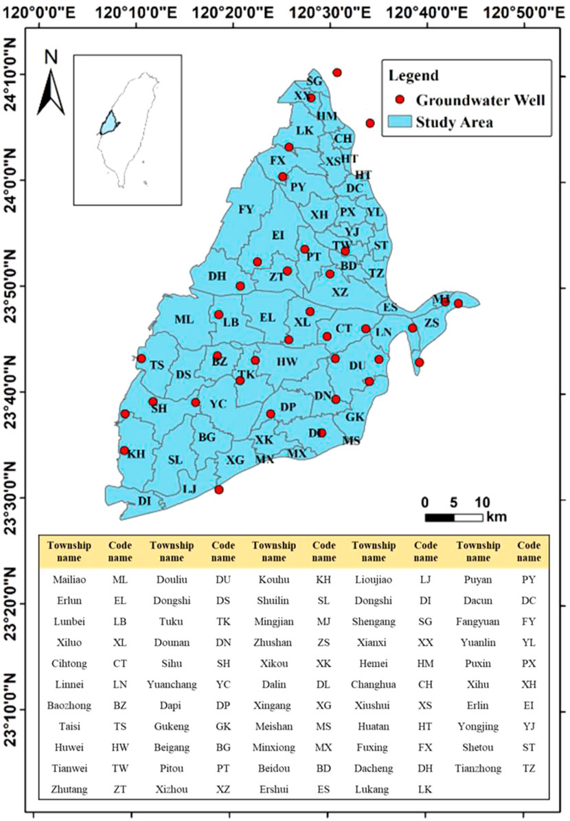
FIGURE 1. Geographical distribution of groundwater observation wells in the Choushui River Alluvial Fan.
This study collected the monthly average GWLs in 35 observation wells in the first aquifer in the study area from 1999 to 2019 from the Water Resources Agency of the Ministry of Economic Affairs. The spatial distribution of GWLs were interpolated to obtain the GWLs of each township during dry and wet seasons using ordinary kriging. Slope (S) has significantly spatial interactions with GWLs (Mulyadi et al., 2020), and drainage density (Dd) indicates the regional drainage conditions depending on the both climate and physical characteristics (Parizi et al., 2020). These two factors were calculated from the 40-m layer of the digital elevation model (DEM) in the ArcGIS software. Normalized difference vegetation index (NDVI) which is often used to assess the growth of green vegetation in the specific area, and the correlation with GWL was also pointed out (Xu et al., 2019; Parizi et al., 2020; Sharma et al., 2021). Monthly satellite images of Landsat 5, Landsat 7, and Landsat 8 with a resolution of 30 m from 1999 to 2019 were obtained from the United States Geological Survey (USGS) website (https://www.usgs.gov/). Precipitation is the main source of groundwater recharge, and monthly precipitation (P) grid data with the resolution of 5 km was from the Taiwan Climate Change Projection Information and Adaptation Knowledge Platform (TCCIP) (https://tccip.ncdr.nat.gov.tw/) from 1999 to 2019. Actual evapotranspiration (AET) and Soil moisture (SM) with a resolution of 4 km from 1999 to 2019 were collected from TerraClimate dataset. It combined the climatically aided interpolation and high-spatial resolution climatological normal from the WorldClim dataset to provide a dataset featuring the monthly climate and climatic water balance for global terrestrial surfaces (http://www.climatologylab.org/terraclimate.html). The two data were adjusted to a resolution of 4 km in this study.
The study explored the variation of GWL and used the Mann–Kendall method to evaluate the long-term GWL trend in the Choushui River alluvial fan at month, season, and wet-and-dry season scales from 1999 to 2019 at the significant level of 0.05. The GWLs decrease in all months. February, March, April, May, November, and December show a significant decrease in GWL, and April is the month with the most significant decrease in GWL (Z value = −2.14). For the season scale, all seasons show a decrease in GWL. There are significant decreases of GWL in spring and winter, and spring has the most significant decrease (Z value = −2.33). The GWL during the dry and wet seasons shows that the dry season has a significant decrease in GWL (Z value = −2.39). The annual average change of the GWL in the Choushui River alluvial fan (Z value = −3.81) also has a significant decrease trend. Results show that the GWL of the alluvial fan of Choushui River is facing a serious decrease.
The GWL of the Choushui River alluvial fan decreased from 1999 to 2019, with the highest average from August to October and the lowest from March to June. The seasonal GWL decreases from autumn, summer, winter, and spring in most years, while P shows that the precipitation is concentrated in summer, followed by spring. Previous study also showed a 3-4 lag time between the precipitation and the groundwater level in the Choushui River alluvial fan (Chang, 2009). Although precipitation such as plum rains and typhoons recharge groundwater in June, the GWL does not reach its peak until approximately September to December, which is during autumn. The changes in the GWL during the dry and wet seasons are similar and consistent in most years.
The spatial distributions of the GWL trend in the Choushui River alluvial fan during dry and wet seasons are shown in Figure 2. There is a significant decrease in GWL in the central area of the alluvial fan, including Baozhong (BZ), Dongshi (DS), Tuku (TK), Yuanchang (YC), Sihu (SH), and the townships with higher elevation including the of Zhushan (ZS), Ershui (ES), and Linnei (LN) during both dry and wet seasons. However, the GWL has a significant increase in the northern study area. These results indicate that the spatial distributions of the GWL trend in the dry and wet seasons are similar. Interestingly, the region with significantly decreasing GWL is consistent with the region (particularly in Baozhong (BZ) and Yuanchang (YC)) with the most serious accumulated land subsidence from 1992 to 2020 obtained from the Water Resources Information Service Platform (https://gic.wra.gov.tw/Gis/Map).
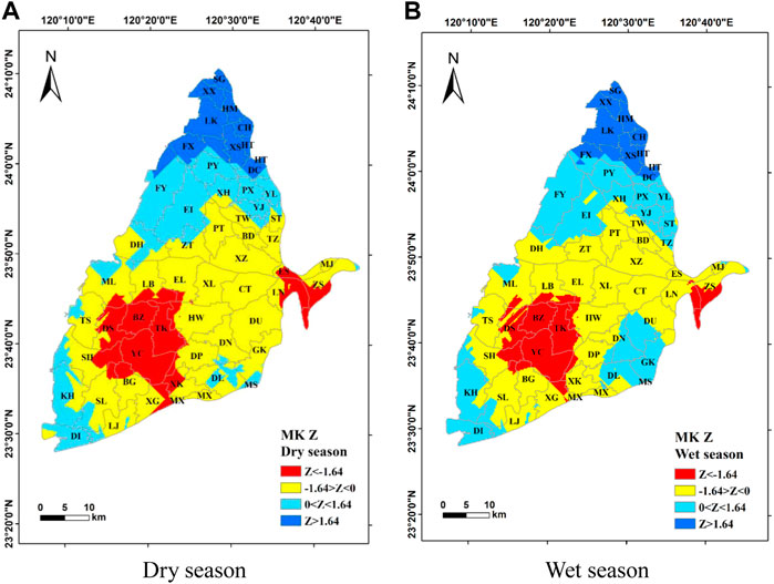
FIGURE 2. Spatial distribution of the Z values obtained from the Mann–Kendall method of the Choushui River Alluvial Fan. (A) Dry season. (B) Wet season.
GWL is the dependent variable of this study. The GWL of the Choushui River alluvial fan varies from −4.1 to 149.4 m in the dry season with an average of 26.6 m, while it varies from −4.1 to 150.5 m with an average of 27.0 m in the wet season. The difference of GWL in the wet and dry seasons is insignificant. In terms of spatial distribution, the GWL decreases from east to west due to the difference in elevation which is also shown in the distribution of slope. In addition, since the overall terrain is relatively flat, it shows that approximately 60% of the GWL in the study area is less than 15 m, as shown in Figure 3.
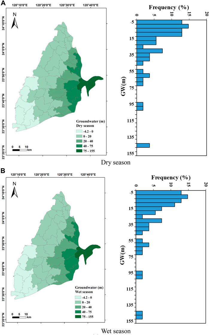
FIGURE 3. Spatial distribution and statistics of groundwater level (GWL) in the Choushui River Alluvial Fan. (A) Dry season. (B) Wet season.
The independent variables in this study include slope (S), drainage density (Dd), normalized difference vegetation index (NDVI), precipitation (P), wetness index (WI), and soil moisture (SM). The statistics of each variable are summarized in Table 2. The S varies from 0.29° to 4.22° with an average of 0.78°, and approximately 70% of the values are below 0.4°, indicating that the overall study area is relatively gentle. The spatial distribution of S shows a decrease from the east to the west in the study area (Figure 4). Dd ranges from 0 to 0.9 km/km2 with an average of 0.19 km/km2. Approximately 30% of the Dd is less than 0.05 km/km2, indicating that the study area is poorly drained. Dd may be decreased with lower amount of precipitation, lower infiltration rate, steeper slope, and more impermeable surfaces. The spatial distribution of Dd shows that it is lower in the northeast and higher in the east of the study area (Figure 5). The unevenly distribution demonstrates that different physical characteristics control the Dd in different areas. NDVI in the dry and wet seasons varies from −0.06 to 0.18 with an average value of 0.07 and from −0.01 to 0.25 with an average value of 0.09, respectively (Figure 6). In the dry season, 40% of the total value ranges from 0.04 to 0.08, while 30% of the total value ranges from 0.06 to 0.08 in the wet season. The overall value is not high and depends on the field crops, water body, and artificial construction. The National Land Use Investigation Map from the Water Resources Information Service Platform (https://gic.wra.gov.tw/gis/) shows that the vegetation type is mainly agriculture rather than forests. The spatial distribution of NDVI shows that it is higher in the southeast of the study area during the dry season, while it decreases toward the west and has negative values in some towns along the coast. The spatial distribution of NDVI in the wet season shows that Gukeng (GK) Township in the southeast of the study area has the highest NDVI value. Except for the Kouhu (KH) Township on the southwestern coast, the overall townships have positive NDVI. It demonstrates obviously seasonal difference of NDVI is mainly concentrated in the coastal area and that the plain areas may be affected by changes in planted crops.
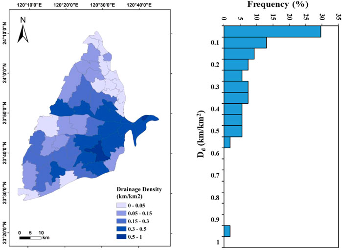
FIGURE 5. Spatial distribution and statistics of drainage density (Dd) in the Choushui River Alluvial Fan.
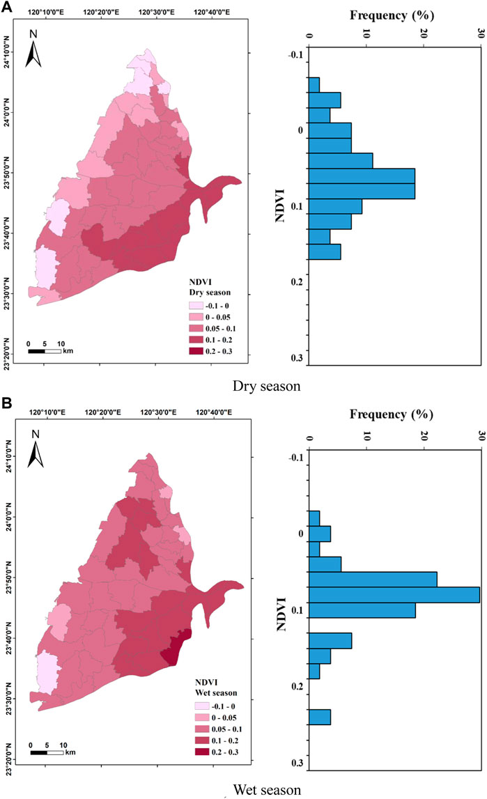
FIGURE 6. Spatial distribution and statistics of normalized difference vegetation index (NDVI) in the Choushui River Alluvial Fan. (A) Dry season. (B) Wet season.
P in the dry season and wet season ranged from 26.3 to 43.6 mm/month with an average of 34.5 mm/month and from 163.2 to 337 mm/month with an average value of 211 mm/month, respectively (Figure 7). In the dry season, 30–40 mm/month accounted for more than 70% of the total value, while the distribution is relatively even in the wet season. These results indicate that P in the study area is exceptionally distinct between dry and wet seasons. The spatial distribution of P in the dry season shows that the P is the highest in the northeast of the study area and gradually decreases toward the southwest; the spatial distribution in the west season decreases from the southeast to the northwest due to the topography and monsoon climate. Wetness Index (WI) is the ratio of rainfall to evapotranspiration (Fu et al., 2019), previous studies also suggested its direct effect on groundwater (Asoka et al., 2021; Wu et al., 2021). Its distribution is similar to that of P (Figure 8). The WI ranged from 0 to 0.81 in the dry season with an average of 0.74, while it ranged from 0 to 2.31 with an average of 1.58 in the wet season. The distributions of WI in the dry and wet seasons are relatively concentrated with more than 80% in the range of 0.7–0.8 and 1.3–1.8, respectively. The spatial distribution of WI in the dry season shows that the values are higher toward the east of Erlin (EI) Township, and it gradually decreases from the north to south. The spatial distribution of WI in the wet season is higher in the east of the research area, and it gradually decreases toward the west of the study area. It suggests that the actual evapotranspiration just has slight difference in the study area. The SM value in the dry season is in the range of 0–24.6 mm with an average of 17.9 mm of which 15–20 mm accounts for 70% of total data. The SM value in the wet season is in the range of 0–73 mm with an average of 68.9 mm of which more than 90% of the values are in the range of 65–75 mm. When the SM is higher than the maximum soil water holding capacity, it will infiltrate into groundwater, affecting the GWL (Asoka & Mishra, 2021). Results show that high SM in the wet season may exceed the maximum soil water holding capacity faster and then infiltrate into the groundwater, thereby affecting the GWL more effectively. In Figure 9, the spatial distribution of SM in the dry season shows that it is higher in the northern and eastern study area, and it gradually decreases toward the south. The SM in the wet season shows that it is also higher in the northern towns while it is lower in the southwestern coast.
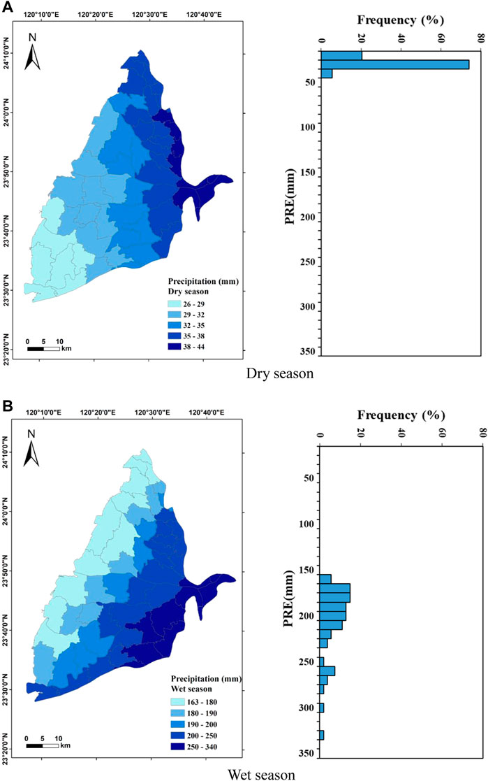
FIGURE 7. Spatial distribution and statistics of precipitation (P) in the Choushui River Alluvial Fan. (A) Dry season. (B) Wet season.
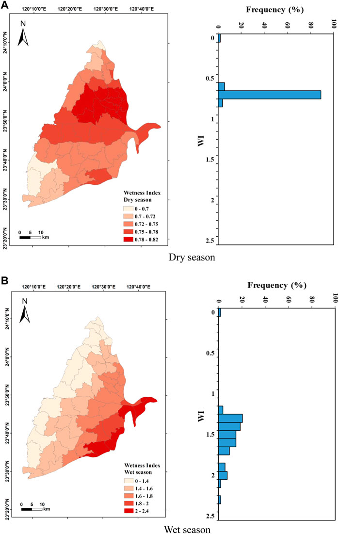
FIGURE 8. Spatial distribution and statistics of wetness index (WI) in the Choushui River Alluvial Fan. (A) Dry season. (B) Wet season.
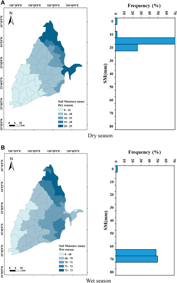
FIGURE 9. Spatial distribution and statistics of soil moisture (SM) in the Choushui River Alluvial Fan. (A) Dry season. (B) Wet season.
This study uses global and local Moran’s I indices to analyze the spatial characteristics of GWL in dry and wet seasons in each township of the Choushui River alluvial fan. The global Moran’s I indices for the dry and wet seasons are 0.813 and 0.811, respectively, indicating that the variable has significant positive spatial correlations in both seasons. The local Moran’s I indices in the dry and wet seasons show that they have the same local spatial distribution. The high GWL towns are adjacent to the other high GWL towns, and the low GWL towns are adjacent to the other low GWL towns. The townships of Tianzhong (TZ), Ershui (ES), Mingjian (MJ), Zhushan (ZS), Linnei (LN), and Cihtong (CT) that are situated at the top of the Choushui River alluvial fan show “HH” clusters spatially, indicating that these townships that have high GWL values are adjacent to other towns with similar high GWL values. Townships spatially classified as “LL” clusters have lower GWL values and are adjacent to the townships with similar low GWL values. There is no significant difference in the spatial distribution of GWL between dry and wet seasons (Figure 10). It describes that the GWLs spatially have great hydrological connectivity in the Choushui River alluvial fan.
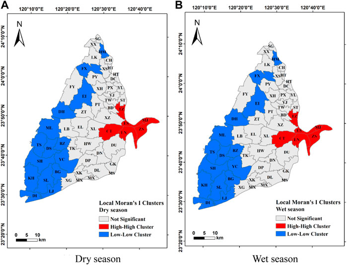
FIGURE 10. Spatial distribution of the local Moran’s I index in the Choushui River Alluvial Fan. (A) Dry season. (B) Wet season.
There are obvious differences in P, AET, and SM between dry and wet seasons in this study area, and thus the natural factors mainly affecting the GWL during dry and wet seasons are also different. The effects of various factors on the GWL values in dry and wet seasons are discussed below. AIC and R2 were used to identify the most important combination of influencing factors in wet and dry seasons. Results show that Dd, S, NDVI, and P influence the GWL during the dry season, and Dd, S, NDVI, and WI influence the GWL during the wet season. These results are shown in Table 3.

TABLE 3. Combined results of influencing factors during dry and wet seasons in the geographically weighted regression model.
Results show that the local R2 of the selected combined model in the dry season ranges from 0.81 to 0.84, indicating that the combination of selected factors has a good fit for the model. The optimal model has the corrected R2 value of 0.86 and the AIC value of 440. Among the standard deviations of the combined model, only the standard deviation of Mingjian (MJ) Township at the top of the alluvial fan exceeds 2.5, and all the other areas are within the normal standard deviation range. This shows that the estimates of coefficient are reliable and that no serious multilinearity problem exists (Figure 11A). In this regression model, the local R2 is an important variable, and its spatial distribution gradually decreases from the east of the study area, where it achieves the highest value at the top of the alluvial fan, to the west of the study area, that is, the tail of the alluvial fan (Figure 11B).
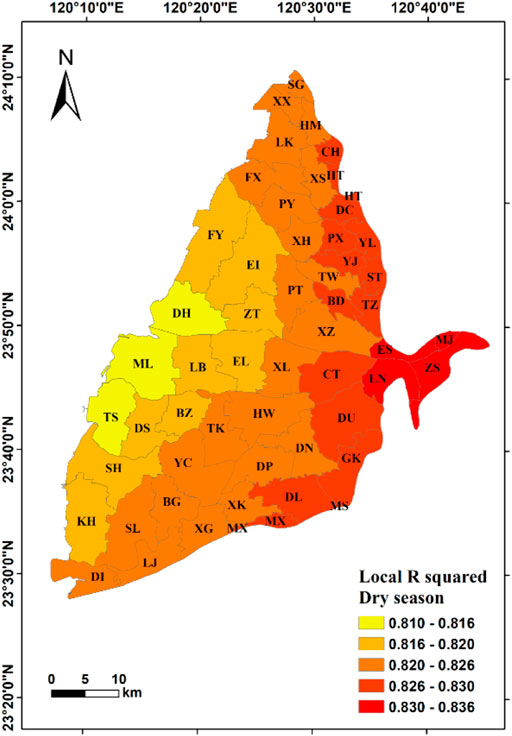
FIGURE 11. Results of geographically weighted regression model during the dry season (influencing factors: Dd, S, NDVI, and P).
The selected factors indicate that all the townships in the study area are significantly positively correlated with the GWL, as shown in Table 4. In Figure 12, the spatial distributions of coefficient of the factors show that the coefficient of Dd is the maximum in the northeast of the study area, and it gradually decreases toward the southwest. The coefficient of S gradually increases from the east (the top of the alluvial fan) to the west (the tail of the alluvial fan), and the value is the highest at the tail of the alluvial fan. The coefficient of NDVI is the maximum in the northern study area and gradually decreases toward the south. The coefficient of P gradually decreases from the east (the top of the alluvial fan) to the west (the tail of the alluvial fan). In overall directions of coefficient distribution, Dd tends to be consistent with NDVI, while S tends to be consistent with precipitation. It demonstrates that this relationship between Dd and NDVI may reflect the main influence on the regional drainage condition, and affecting the GWL the most in the northern region. The inverse tendency between S and P shows that the slope and the precipitation have a greater effect on the tail and the top of the alluvial fan, respectively. It may suggest that the groundwater level in a steeper region mainly controlled by the amount of precipitation in our study area.

TABLE 4. The coefficient values of influencing factors of the geographically weighted regression model during the dry season.
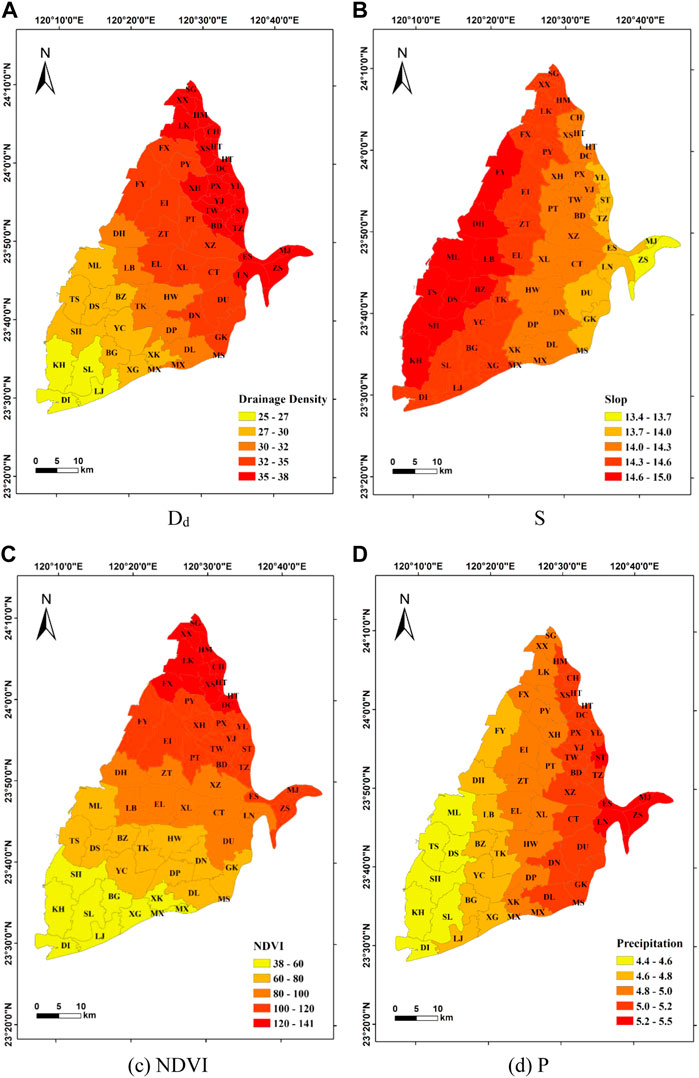
FIGURE 12. Spatial distribution of factor coefficients of the geographically weighted regression model during the dry season. (A) Dd (B) S (C) NDVI (D) P.
The GWR analysis in the wet season shows that the local R2 range of the selected combined model is 0.65–0.85, and the optimal model has the corrected R2 value of 0.82 and the AIC value of 458. Similar to the result in the dry season, only the townships of Mingjian (MJ) and Ershui (ES) in the east (the top of the alluvial fan) have standard deviations exceeding 2.5, and all the other areas are within the normal standard deviation range (Figure 13A). The spatial distribution of the local R2 value of the combined model is the lowest in the middle of the alluvial fan, and it increases toward the south and the north (Figure 13B). S and WI have a significant positive correlation with the GWL in the study area. Dd and NDVI have both significant positive and negative correlation coefficient values, indicating that they are inconsistent with the GWL in the townships (Table 5).
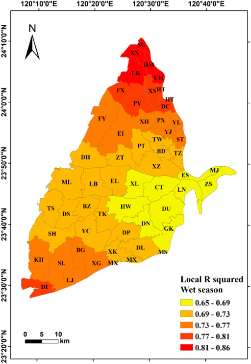
FIGURE 13. Results of geographically weighted regression model during the wet season (influencing factors: Dd, S, NDVI, and WI).

TABLE 5. The coefficient values of influencing factors of the geographically weighted regression model during the wet season.
]In Figure 14, the coefficient values of Dd is the lowest in the northwest and increases toward the southeast. The coefficient values of S are the lowest in the townships of Shengang (SG), Xianxi (XX), and Hemei (HM), and Changhua City (CH) in the northern study area, and it increases toward the south and decreases again in the townships of Kouhu (KH) and Dongshi (DI). The coefficient values of NDVI in the townships of Dounan (DN), Dapi (DP), Dalin (DL), Minxiong (MX), and Gukeng (GK) have the largest negative correlation with the GWL, while the highest coefficient values of NDVI are in the northeast and southwest of the study area. The coefficient values of WI gradually decrease from the north to the south of the study area. Dd tends to be consistent with WI, while S tends to be consistent with NDVI. These is totally different from the results in the dry season. The inverse tendency between Dd and WI shows that the effective precipitation and the regional drainage condition has the most influence on the north and the south of study area, respectively. In addition, the coefficient tendency of Dd may be related to the negative correlation between NDVI and groundwater level. The opposite radial tendency between slope and NDVI may describe that land cover type and slope have greater influence on the southeast of study area. This shows that the groundwater response mechanism is more complex in the wet season, and it may be related to crop growth in local areas.
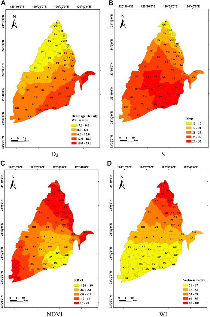
FIGURE 14. Spatial distribution of factor coefficients of the geographically weighted regression model during the wet season. (A) Dd (B) S (C) NDVI (D) WI.
A GWR model was established based on data of the Choushui River alluvial fan from 1999 to 2019. We explored the spatial correlation between natural factors and the GWL during dry and wet seasons. We also analyze the trend on the GWL time series using the Mann–Kendall trend test, using the Moran’s I index to understand the spatial aggregation characteristics of the GWL. According to the Mann–Kendall test, the GWL of the Choushui River alluvial fan is significantly decreasing at month, season, and dry- and wet-season scale. The distribution of the trend in the GWL during dry and wet seasons is consistent. The global Moran’s I indices of GWL show significant positive spatial correlations in both dry and wet seasons. Local Moran’s I indices also show that the high GWL towns are adjacent to other high GWL towns, while the low GWL towns are adjacent to other low GWL towns. The GWR model analysis shows that the changes in GWL in the research area during the dry season are affected by Dd, S, NDVI, and P, while the changes in GWL in the wet season are affected by Dd, S, NDVI, and WI. The tendencies of coefficient distribution have the great difference in both seasons. In the dry seasons, the relationship among natural factors and GWL are easily understood, but the more complex groundwater response mechanism exists in the wet seasons. This might be caused by crop growth or other land use change in local areas. These results could be provided as references for future regional water resource utilization and management.
The original contributions presented in the study are included in the article/Supplementary Material; further inquiries can be directed to the corresponding author.
Material preparation, investigation, data collection and curation were performed by J-CC. Conceptualization, data analysis, visualization and the original draft was performed by C-CH and H-YC. Supervision and Writing—reviewing and; editing was performed by H-FY. All authors commented on previous versions of the manuscript and approved the final manuscript.
The authors declare that the research was conducted in the absence of any commercial or financial relationships that could be construed as a potential conflict of interest.
All claims expressed in this article are solely those of the authors and do not necessarily represent those of their affiliated organizations, or those of the publisher, the editors and the reviewers. Any product that may be evaluated in this article, or claim that may be made by its manufacturer, is not guaranteed or endorsed by the publisher.
Ainiwaer, M., Ding, J., Wang, J., and Nasierding, N. (2019). Spatiotemporal dynamics of water table depth associated with changing agricultural land use in an arid zone oasis. Water 11 (4), 673.
Asoka, A., and Mishra, V. (2021). A strong linkage between seasonal crop growth and groundwater storage variability in India. J. Hydrometeorol. 22 (1), 125–138.
Boots, B. (2003). Developing local measures of spatial association for categorical data. J. Geogr. Syst. 5 (2), 139–160. doi:10.1007/s10109-003-0110-3
Brunsdon, C., Fotheringham, A. S., and Charlton, M. E. (1996). Geographically weighted regression: A method for exploring spatial nonstationarity. Geogr. Anal. 28 (4), 281–298.
Brunsdon, C., Fotheringham, S., and Charlton, M. (1998). Geographically weighted regression. J. R. Stat. Soc. Ser. D (The Statistician) 47 (3), 431–443.
Burke, J. J., and Moench, M. H. (2000). Groundwater and society: resources, tensions and opportunities. Themes in groundwater management for the twenty-first century. New York: Department of International Economic and Social Affairs, Statistical Office.
Chang, L.-C. (2009). Hydrogeology investigation and groundwater resource assessment for Taiwan : Groundwater recharge estimation and model simulation.1/4
Chen, Y.-A., Chang, C.-P., Hung, W.-C., Yen, J.-Y., Lu, C.-H., and Hwang, C. (2021). Space-time evolutions of land subsidence in the Choushui River alluvial fan (taiwan) from multiple-sensor observations. Remote Sensing 13 (12), 2281.
Chu, H.-J., and Burbey, T. J. (2022). Estimating future (next-month’s) spatial groundwater response from current regional pumping and precipitation rates. Journal of Hydrology 604, 127160.
Duran-Llacer, I., Munizaga, J., Arumí, J. L., Ruybal, C., Aguayo, M., Sáez-Carrillo, K., et al. (2020). Lessons to be learned: Groundwater depletion in Chile’s Ligua and Petorca watersheds through an Interdisciplinary approach. Water 12 (9), 2446.
Ebrahimi, A., Nazemosadat, S., Motamedvaziri, B., and Ahmadi, H. (2021). Land use-land cover change and its relationships with the groundwater table and the plants’ altitudinal zones: A case study of arsanjan county, Iran. Iranian Journal of Science and Technology, Transactions of Civil Engineering 45 (3), 1891–1907.
Foster, S., Chilton, J., Nijsten, G.-J., and Richts, A. (2013). Groundwater—A global focus on the ‘local resource. Current opinion in environmental sustainability 5 (6), 685–695.
Fu, G., Crosbie, R. S., Barron, O., Charles, S. P., Dawes, W., Shi, X., et al. (2019). Attributing variations of temporal and spatial groundwater recharge: A statistical analysis of climatic and non-climatic factors. Journal of Hydrology 568, 816–834.
Galloway, D. L., and Burbey, T. J. (2011). Regional land subsidence accompanying groundwater extraction. Hydrogeology Journal 19 (8), 1459–1486.
Haddad, M., Feitelson, E., and Arlosoroff, S. (2001). “The management of shared aquifers,” in Management of shared groundwater resources (Springer), 3–23.
Hsu, W.-C., Chang, H.-C., Chang, K.-T., Lin, E.-K., Liu, J.-K., and Liou, Y.-A. (2015). Observing land subsidence and revealing the factors that influence it using a multi-sensor approach in Yunlin County, Taiwan. Remote Sensing 7 (6), 8202–8223.
Hung, W.-C., Hwang, C., Chang, C.-P., Yen, J.-Y., Liu, C.-H., and Yang, W.-H. (2010). Monitoring severe aquifer-system compaction and land subsidence in Taiwan using multiple sensors: Yunlin, the southern Choushui River Alluvial Fan. Environmental Earth Sciences 59 (7), 1535–1548.
Hurvich, C. M., Simonoff, J. S., and Tsai, C. L. (1998). Smoothing parameter selection in nonparametric regression using an improved Akaike information criterion. Journal of the Royal Statistical Society Series B (Statistical Methodology) 60 (2), 271–293.
Hwang, C., Yang, Y., Kao, R., Han, J., Shum, C., Galloway, D. L., et al. (2016). Time-varying land subsidence detected by radar altimetry: California, taiwan and north China. Scientific Reports 6 (1), 1–12.
Jeanne, P., Farr, T. G., Rutqvist, J., and Vasco, D. W. (2019). Role of agricultural activity on land subsidence in the San Joaquin Valley, California. Journal of Hydrology 569, 462–469.
Kløve, B., Ala-Aho, P., Bertrand, G., Boukalova, Z., Ertürk, A., Goldscheider, N., et al. (2011). Groundwater dependent ecosystems. Part I: Hydroecological status and trends. Environmental Science & Policy 14 (7), 770–781.
Li, H., Lu, Y., Zheng, C., Zhang, X., Zhou, B., and Wu, J. (2020). Seasonal and inter-annual variability of groundwater and their responses to climate change and human activities in arid and desert areas: A case study in yaoba oasis, northwest China. Water 12 (1), 303.
Lin, M., Biswas, A., and Bennett, E. M. (2020). Socio-ecological determinants on spatio-temporal changes of groundwater in the Yellow River Basin, China. Science of the total environment 731, 138725.
Liu, C. W. (2004). Decision support system for managing ground water resources in the CHOUSHUI River alluvial in taiwan 1. JAWRA Journal of the American Water Resources Association 40 (2), 431–442.
Machard de Gramont, H., Noel, C., Oliver, J., Pennequin, D., Rama, M., and Stephan, R. (2011). Towards a joint management of transboundary aquifer systems. Methodological guidebookCollection ‘À Savoir 3. (available in English and in French).
Maihemuti, B., Simayi, Z., Alifujiang, Y., Aishan, T., Abliz, A., and Aierken, G. (2021). Development and evaluation of the soil water balance model in an inland arid delta oasis: Implications for sustainable groundwater resource management. Global Ecology and Conservation 25, e01408.
Mann, H. B. (1945). Nonparametric tests against trend. Econometrica Journal of the econometric society, 245–259.
Miller, J. A., and Hanham, R. Q. (2011). Spatial nonstationarity and the scale of species–environment relationships in the Mojave Desert, California, USA. International Journal of Geographical Information Science 25 (3), 423–438.
Mulyadi, A., Dede, M., and Widiawaty, M. A. (2020). “Spatial interaction of groundwater and surface topographic using geographically weighted regression in built-up area,” in IOP conference series: Earth and environmental science. Paper presented at the.
Odgaard, M. V., Bøcher, P. K., Dalgaard, T., Moeslund, J. E., and Svenning, J.-C. (2014). Human-driven topographic effects on the distribution of forest in a flat, lowland agricultural region. Journal of Geographical Sciences 24 (1), 76–92.
Ojeda Olivares, E. A., Sandoval Torres, S., Belmonte Jiménez, S. I., Campos Enríquez, J. O., Zignol, F., Reygadas, Y., et al. (2019). Climate change, land use/land cover change, and population growth as drivers of groundwater depletion in the Central Valleys, Oaxaca, Mexico. Remote Sensing 11 (11), 1290.
Parizi, E., Hosseini, S. M., Ataie-Ashtiani, B., and Simmons, C. T. (2020). Normalized difference vegetation index as the dominant predicting factor of groundwater recharge in phreatic aquifers: Case studies across Iran. Scientific Reports 10 (1), 1–19.
Sharma, A. K., Hubert-Moy, L., Buvaneshwari, S., Sekhar, M., Ruiz, L., Moger, H., et al. (2021). Identifying seasonal groundwater-irrigated cropland using multi-source NDVI time-series images. Remote Sensing 13 (10), 1960.
Siebert, S., Burke, J., Faures, J.-M., Frenken, K., Hoogeveen, J., Döll, P., et al. (2010). Groundwater use for irrigation—A global inventory. Hydrology and Earth System Sciences 14 (10), 1863–1880.
Taylor, R. G., Scanlon, B., Döll, P., Rodell, M., Van Beek, R., Wada, Y., et al. (2013). Ground water and climate change. Nature climate change 3 (4), 322–329.
Van Huijgevoort, M. H., Voortman, B. R., Rijpkema, S., Nijhuis, K. H., and Witte, J.-P. M. (2020). Influence of climate and land use change on the groundwater system of the veluwe, The Netherlands: A historical and future perspective. Water 12 (10), 2866.
Wada, Y., Van Beek, L. P., Van Kempen, C. M., Reckman, J. W., Vasak, S., and Bierkens, M. F. (2010). Global depletion of groundwater resources. Geophysical research letters 37 (20).
Wang, T.-Y., Wang, P., Zhang, Y.-C., Yu, J.-J., Du, C.-Y., and Fang, Y.-H. (2019). Contrasting groundwater depletion patterns induced by anthropogenic and climate-driven factors on Alxa Plateau, northwestern China. Journal of Hydrology 576, 262–272.
Wu, Y., Yang, G., Tian, L., Gu, X., Li, X., He, X., et al. (2021). Spatiotemporal variation in groundwater level within the Manas River Basin, Northwest China: Relative impacts of natural and human factors. Open geosciences 13 (1), 626–638.
Xia, J., Wu, X., Zhan, C., Qiao, Y., Hong, S., Yang, P., et al. (2019). Evaluating the dynamics of groundwater depletion for an arid land in the Tarim Basin, China. Water 11 (2), 186.
Xinqiang, D., Kaiyang, C., and Xiangqin, L. (2020). Characteristics and causes of groundwater dynamic changes in naoli river plain, northeast China. Water Supply 20 (7), 2603–2615.
Xu, W., and Su, X. (2019). Challenges and impacts of climate change and human activities on groundwater-dependent ecosystems in arid areas–A case study of the Nalenggele alluvial fan in NW China. Journal of Hydrology 573, 376–385.
Yang, Y.-J., Hwang, C., Hung, W.-C., Fuhrmann, T., Chen, Y.-A., and Wei, S.-H. (2019). Surface deformation from sentinel-1A InSAR: Relation to seasonal groundwater extraction and rainfall in central taiwan. Remote Sensing 11 (23), 2817.
Keywords: geographically weighted regression model, groundwater level, normalized difference vegetation index, Choushui river, Taiwan
Citation: Yeh H-F, Chang J-C, Huang C-C and Chen H-Y (2022) Spatial correlation of groundwater level with natural factors using geographically weighted regression model in the Choushui River Alluvial Fan, Taiwan. Front. Earth Sci. 10:977611. doi: 10.3389/feart.2022.977611
Received: 24 June 2022; Accepted: 30 August 2022;
Published: 15 September 2022.
Edited by:
Venkatesh Merwade, Purdue University, United StatesReviewed by:
Wei Xu, Shenyang Agricultural University, ChinaCopyright © 2022 Yeh, Chang, Huang and Chen. This is an open-access article distributed under the terms of the Creative Commons Attribution License (CC BY). The use, distribution or reproduction in other forums is permitted, provided the original author(s) and the copyright owner(s) are credited and that the original publication in this journal is cited, in accordance with accepted academic practice. No use, distribution or reproduction is permitted which does not comply with these terms.
*Correspondence: Hsin-Fu Yeh, aGZ5ZWhAbWFpbC5uY2t1LmVkdS50dw==
Disclaimer: All claims expressed in this article are solely those of the authors and do not necessarily represent those of their affiliated organizations, or those of the publisher, the editors and the reviewers. Any product that may be evaluated in this article or claim that may be made by its manufacturer is not guaranteed or endorsed by the publisher.
Research integrity at Frontiers

Learn more about the work of our research integrity team to safeguard the quality of each article we publish.