The Water Cycle of the Baltic Sea Region From GRACE/GRACE-FO Missions and ERA5 Data

The water cycle of the Baltic Sea has been estimated from the Gravity Recovery and Climate Experiment (GRACE) and the GRACE Follow-On satellite time-variable gravity measurements, and precipitation and evaporation from ERA5 atmospheric reanalysis data for the periods 06/2002 to 06/2017 and 06/2018 to 11/2021. On average, the Baltic Sea evaporates 199 ± 3 km³/year, which is overcompensated with 256 ± 6 km³/year of precipitation and 476 ± 17 km³/year of water from land. This surplus of freshwater inflow produces a salty water net outflow from the Baltic Sea of 515 ± 27 km³/year, which increases to 668 ± 32 km³/year when the Kattegat and Skagerrak straits are included. In general, the balance among the fluxes is not reached instantaneously, and all of them present seasonal variability. The Baltic net outflow reaches an annual minimum of 221 ± 79 km³/year in September and a maximum of 814 ± 94 km³/year in May, mainly driven by the freshwater contribution from land. On the interannual scale, the annual mean of the Baltic net outflow can vary up to 470 km³/year from year to year. This variability is not directly related to the North Atlantic Oscillation during wintertime, although the latter is well correlated with net precipitation in both continental drainage basins and the Baltic Sea.

Introduction

The hydrological or water cycle refers to the continuous movement of water in the atmosphere, continents, oceans, and among them. It regulates the weather and determines the availability of fresh water, which is vital for both human and ecosystem life. Understanding the water cycle of a region is crucial to manage freshwater resources and then human and natural life. As the hydrological cycle is both cause and consequence of the climate of any region, it is vulnerable to climate change. At present, the global hydrological cycle is intensifying (Durack et al., 2012; Markonis et al., 2019), which is unsurprising under the ongoing global warming scenario (Held and Soden, 2006; Huntington, 2006; Greve et al., 2014). In addition, the monitoring of water cycles and their time evolution should be done at a regional scale since the response of each region to changes in the hydrological cycle is different. Giorgi (2006) estimated the vulnerability of several regions based on results from a multi-model ensemble of climate change simulations. The most vulnerable regions are the Mediterranean and northeastern Europe regions. The second most vulnerable regions are a tropical region (Central America) and three regions with high latitude cold climate (northern Europe, Greenland, and Northern Asia). Here, we study the hydrological cycle of the Baltic Sea, in northern Europe, following the same approach of a previous study focused on the Mediterranean-Black Sea system (García-García et al., 2022).

The Baltic Sea is an intracontinental and semi-enclosed basin of ∼ 380·10³ km² surrounded by nine countries: Denmark, Germany, Poland, Lithuania, Latvia, Estonia, Russia, Finland, and Sweden. It is a shallow sea with 55 m of average depth and 459 m of maximum depth (Daraghi et al., 2017). The continental drainage region is inhabited by ∼ 85 million people, whose livelihood largely depends on the sea. The Baltic Sea is connected to the North Atlantic Ocean at the North Sea through three consecutive straits. From the Baltic Sea to the North Sea, we find the following: 1) the Danish straits, which consist of three small straits: the Great Belt (60 km long and 16–32 km wide), the Little Belt (50 km long and 0.8–28 km wide), and the Øresund (118 km long and 4–28 km wide); 2) the Kattegat Strait (220 km long and 60–142 km wide); and 3) Skagerrak Strait (240 km long and 130–145 km wide) (Figure 1). Vertically, the Baltic Sea exchanges fresh water with the atmosphere via precipitation (P) and evaporation (E). Horizontally, the Baltic Sea receives fresh water from the surrounding lands (R), where the excess of P over E that is not stored on land must flow to the sea. Then, R accounts for river runoff, but also for surface runoff outside the course of the rivers and submarine groundwater discharge to the ocean. River runoff for this region has been previously estimated, from in situ observations and models, with values between 428 and 522 km³/year from different methodologies, data sets, and periods of time (see Table 1). Also horizontally, the Baltic Sea exchanges salty water with the North Sea in a way that can be approximated by a two-layer model: at the bottom layer, the North Sea introduces saltier (and denser) water into the Baltic Sea, while at the top one, fresher (and less dense) water flows in the opposite sense (e.g., The BACC Author Team, 2008; Hanninen et al., 2021). Outflow is lighter than inflow because P and R exceed E in the Baltic Sea freshening the water. The imbalance between the inflow and the outflow results in a net outflow leaving the Baltic Sea, denoted by N, that oscillates between 311 and 621 km³/year, as estimated from current and sea level observations, and numerical models (see Table 2). This situation opposes the one found in another semi-enclosed sea, the Mediterranean Sea, where E exceeds P and R, and highly saline water sinks to the bottom and then is transported to the North Atlantic Ocean through the Strait of Gibraltar, while less salty water flows near the surface in the opposite sense (Jordà et al., 2017, and references therein). The exchange of salty water together with other biogeochemical tracers is important, for example, for the organisms living in the deep waters of the Baltic Sea, which rely on the inflows of extremely salty and oxygenated water from the North Sea (Stramska and Aniskiewicz, 2019).

FIGURE 1

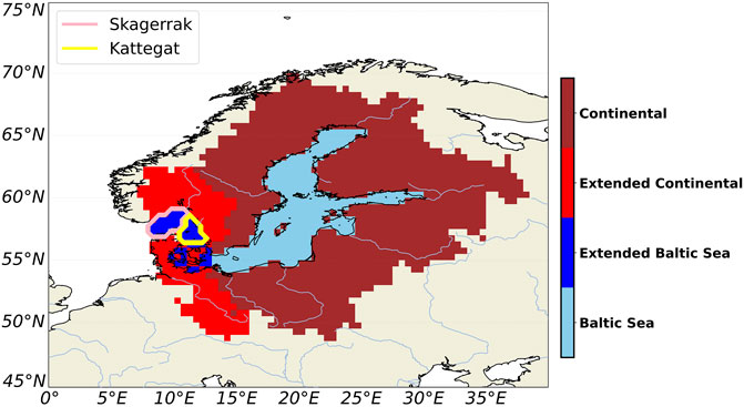
FIGURE 1. Baltic Sea region. Cyan: Baltic Sea; brown: continental basins draining to the Baltic Sea; cyan + blue: the extended Baltic Sea; brown + red: continental basins draining to the extended Baltic Sea. Pink line: boundaries of the Skagerrak strait; yellow line: boundaries of the Kattegat strait.

TABLE 1

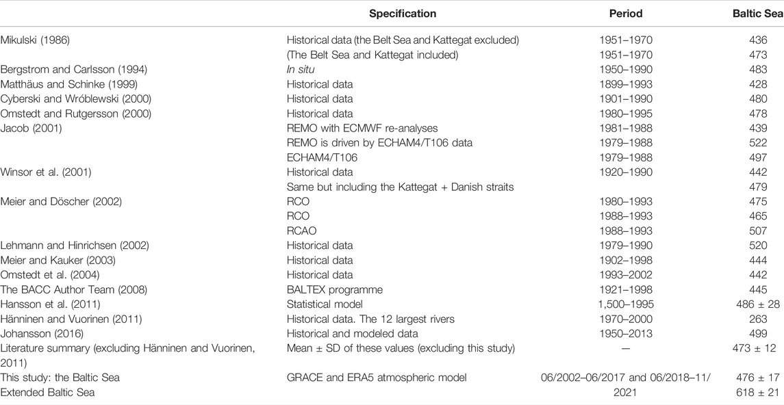
TABLE 1. Reported values of runoff into the Baltic Sea from the literature and estimated R in the present study. Units are km³/year. Acronyms: REMO, Regional Model; ECMWF, European Centre for Medium-Range Weather Forecasts; ECHAM, European Centre Hamburg Model; RCO, Rossby Centre Ocean Model; RCAO, Rossby Centre Atmosphere–Ocean Model; BALTEX, Baltic Sea Experiment; BACC, BALTEX Assessment of Climate Change for the Baltic Sea Basin.

TABLE 2

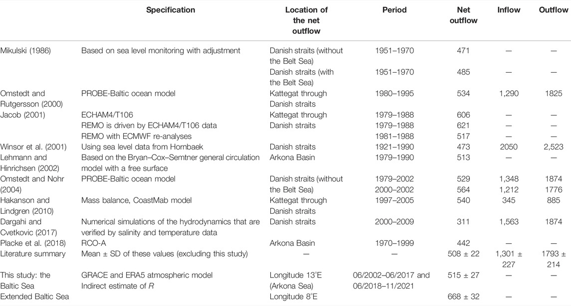
TABLE 2. Reported values of net seawater outflow from the Baltic Sea from the literature and the present study. Outflow means WT leaving the Baltic Sea. The extended Baltic Sea includes the Kattegat and Skagerrak straits. Units are km³/year. Acronyms: PROBE, Program for Boundary Layers in the Environment; CoastMab, a process-based mass-balance model for phosphorus for coastal areas; RCO-A, assimilation/reanalysis setup of the RCO model.

In 2002, the GRACE (Gravity Recovery and Climate Experiment) satellite mission was launched to estimate time-variable gravity data, which is corrected for some known geophysical signals as, for example, solid and ocean tides, pole tides, or gravitational perturbations from the Sun, Moon, and solar system planets. Assuming that the remaining gravity variations are produced by mass variations on the surface of the Earth (such as the water mass transport within the water cycle, the biggest mass variations of the Earth in the intra-annual timescale), the surface mass variation can be uniquely determined (Wahr et al., 1998; Chao, 2005). These data revolutionized the way to study the Earth (see Wouters et al., 2014, and references therein) since it produced a unique tool to understand the water mass transport in the Earth system, and hence the water cycle. In the Baltic region, GRACE data have been used to estimate the variability of the seawater budget, which explained more than half of the sea-level variations (Virtanen et al., 2010), and that of the terrestrial water budget in some coastal points (Pajak and Birylo, 2017). The main contribution of this study is a novel application of the GRACE data to estimate the net seawater mass exchange in the Baltic Sea using the algorithm proposed by García-García et al. (2020) that uses GRACE data to estimate the net water mass transport (WT) among ocean basins and that allows to track the oceanic components of the water cycle. When the algorithm is applied to semi-enclosed basins, it is possible to estimate the water mass exchange between the basin and the open ocean as shown for the Mediterranean Sea by García-García et al. (2022). An additional contribution is the use of GRACE data to estimate the water discharge from the continents in the Baltic Sea, which mainly is runoff. For this second objective, we followed the same methodology used for related problems in other regions. For example, independent of in situ observations, GRACE data have been used to estimate runoff of major river basins such as the Amazon (Syed et al., 2005; Eom et al., 2017), Paraná (Lee et al., 2018), Mississippi (Syed et al., 2005), Yellow River (Li et al., 2016), and smaller river basins (Lorenz et al., 2014). Due to the global nature of GRACE measurements, GRACE data have also been used to estimate the R of whole continents and the R received for whole ocean basins (Syed et al., 2009).

For the net seawater mass exchange in the Baltic Sea, we have used time-variable gravity measurements from GRACE and GRACE Follow-On satellites (GRACE FO), as well as P and E, obtained from ERA5 atmospheric reanalysis data, to estimate the mean values and time-variable evolution of all the WT components involved in the water cycle of the Baltic Sea for the periods 06/2002 to 06/2017 and 06/2018 to 11/2021. GRACE and GRACE FO data are crucial to estimate R and N independently of in situ observations or models. The study is structured as follows: in the Methods and Data section, satellite-based gravimetric and reanalysis data used to study the hydrological cycle are described in detail, together with those methods applied to evaluate seasonal and nonseasonal signals of WT components, and their uncertainties; Results section shows the main results found for all WT terms, including the time mean, the seasonal cycle, and the nonseasonal signal, as well as their connection with the North Atlantic Oscillation; finally, in the Discussion and Conclusion sections the main results are discussed and outlined, respectively.

Methods and Data

This section describes the following: 1) the methodology used to estimate R and N in the Baltic Sea, as well as the theoretical frame to estimate the associated errors; 2) the data used, consisting of time-variable gravity, and P and E atmospheric variables from a reanalysis atmospheric model, as well as the applied corrections.

Methods

The estimation of P, E, R, and N, as well as their time evolution, is key to understanding the regional water cycle. In the Baltic Sea, all WT components are related via the water balance equation:

$dW = P - E + R + N,(1)$

where the new term dW represents the change in water content in the region. According to the equation, positive (negative) values of N represent inflows to (outflows from) the Baltic Sea. If P, E, and dW are known, then R and N can be estimated in a two-step process (García-García et al., 2020; 2022). First, Eq. 1 is applied to the continental catchment region draining to the Baltic Sea, which is identified according to the global continental runoff pathway scheme (Oki and Sud, 1998). Note that in this case N = 0 and R is estimated as a residual. Second, Eq. 1 is applied to the Baltic Sea and N is estimated as a residual.

For each WT time series, the following harmonic regression model with linear trend, and annual and semiannual components has been considered (e.g., Jin and Feng, 2013; Fatolazadeh and Goïta, 2021):

$C_t=p_0+p_1·t+A_a \cos \left({\omega }_a·t-{\mathrm{\varphi }}_a\right)+A_{sa} \cos \left({\omega }_{sa}·\mathrm{t}-{\mathrm{\varphi }}_{sa}\right), (2)$

where t represents time, C_t is the value of the time series of interest at time t, (ω, A, ϕ) = (frequency, amplitude, phase), and the suffixes a and sa denote annual and semiannual terms, respectively. Note that ${\varphi }_a$ determines when the annual maximum is reached, since a degree is roughly equivalent to a day of the year. Using the angle subtraction cosine formula, the model in Eq. 2 can be written as a linear regression model with independent variables: cos (ω_a · t), sin (ω_a · t), cos (ω_sa · t), and sin (ω_sa · t). Then, Eq. 2 can be rewritten as

$C_t={\mathrm{p}}_0+{\mathrm{p}}_1·\mathrm{t}+a_1 \cos \left({\mathrm{\omega }}_a·\mathrm{t}\right)+b_1 \sin \left({\mathrm{\omega }}_a·\mathrm{t}\right)+a_2 \cos \left({\mathrm{\omega }}_{sa}·\mathrm{t}\right)+b_2 \sin \left({\mathrm{\omega }}_{sa}·\mathrm{t}\right),(3)$

where

$a_1=A_a \cos \left({\mathrm{\varphi }}_a\right),b_1=A_a \sin \left({\mathrm{\varphi }}_a\right),(4)$

$a_2=A_{sa} \cos \left({\mathrm{\varphi }}_{sa}\right),b_2=A_{sa} \sin \left({\mathrm{\varphi }}_{sa}\right).(5)$

The parameters p₀, p₁, a₁, b₁, a₂, and b₂ in Eq. 3 are estimated by ordinary least squares. Then, (A_a, ϕ_a) and (A_sa, ϕ_sa) are estimated from Eqs 4, 5, respectively. In particular, we have

$A_a=\sqrt{a_1^2+b_1^2},A_{sa}=\sqrt{a_2^2+b_2^2}.$

The annual component is considered not statistically significant when the p-value for both coefficients a₁ and b₁ in the linear regression in Eq. 3 is greater or equal to 0.05. The same reasoning is used to assess the statistical significance of the semiannual component.

The reported standard deviations (SD) and 95% confidence intervals (CI) for the averages, trends, and seasonal signals of the components of the WT, as well as for correlations, have been evaluated using the stationary bootstrap scheme of Politis and Romano (1994) with the optimal block length selected according to Patton et al. (2009) as well as the percentile method. Note that each time series comprises 221 observations and can be seen as the junction of two evenly spaced time series (with 181 observations from June 2002 to June 2017, and 40 observations from June 2018 to November 2021) separated by a gap of 11 months. Since the stationary bootstrap assumes evenly spaced data, the distributions and the SD of the estimators of the quantities of interest were obtained by applying the bootstrap to the first series (of length 181). In all cases, the distribution of the estimator was approximately normal; thus, the corresponding 95% CI can be obtained as the mean of the bootstrap estimates plus/minus 2 SD. In order to make full use of the data, in the calculation of 95% CI, averages of the bootstrap estimates based on the reduced series (with 181 observations) were replaced by the estimate of the quantity of interest based on the original time series (with 221 observations). To simplify the notation, all results in this study are provided in the form estimate ±SD. The implementation of the stationary bootstrap used here is very similar to the one used in the study by García-García et al. (2020) and García-García et al. (2022), and further details can be found there. The number of bootstrap replications was set to 10,000.

As a sensitivity check, the analysis was repeated including a third cosine term in Eq. 2 to account for the 161-day signal due to the S2 aliasing in the GRACE data. The results of the analysis with and without this additional cosine term were identical.

Data

Net precipitation, P–E, is obtained from the ERA5 reanalysis (Hersbach et al., 2018; data accessed on 26/01/2022), which incorporates observational data into general-circulation modeling supplied by the European Centre for Medium-Range Weather Forecasts (ECMWF). It provides monthly (and hourly) coverage of all continents and seas. As data are available in a 0.25° regular grid for 2002–2021, they have been resampled to a 0.5° regular grid by simple averaging to match the spatial resolution of the continental drainage basin data.

Water mass budget variations, dW, are estimated from the RL06 GRACE mascon (mass concentration) v2 solution provided by the Center of Space Research (CSR) at the University of Texas at Austin (Save et al., 2016; Save, 2019; data accessed on 26/01/2022) for the period of May 2002–November 2021. Time series have missing values between the end of the GRACE mission and the beginning of the GRACE FO, that is, from July 2017 to May 2018. Moreover, the values of 12 single months and 5 pairs of consecutive months were missing and have been linearly interpolated. Data are on a 0.25° regular grid, but we have re-gridded them to 0.5° regular grids as we did for P–E. Note that the obtained spatial resolution is still finer than the ∼ 300 km ( ∼ 3° near the Equator) resolution of GRACE, which measures gravity anomalies from month to month with respect to a dynamic geophysical model that accounts for solid and ocean tides, among other factors. Assuming that the gravity changes are produced by mass changes on the Earth’s surface, such as in the oceans, the mascon solution can be interpreted as water mass (W) budget anomalies (Chao, 2016). Time variations of W (that is, dW) are estimated as the discrete central derivative of W,

$dW\left(t\right)=\frac{dW\left(t+1\right)-dW\left(t-1\right)}{2},$

where t refers to any given month. As a result, dW data span from June 2002 to June 2017 and from June 2018 to November 2021. The same months are selected for P–E data.

In the mascon solution, the following usual corrections are applied by CSR to time-variable data, which include measurements from both GRACE and GRACE FO missions: 1) a solution from Satellite Laser Ranging was used to replace the C₂₀ coefficient (Cheng and Ries, 2017); 2) C₃₀ coefficient is also replaced, but only in data from the GRACE FO; 3) an estimate of the degree-1 coefficients was added (Swenson et al., 2008; Sun et al., 2016); 4) a glacial isostatic adjustment correction (GIA) was performed (Peltier et al., 2018). Moreover, we applied the following corrections: 5) the bottom pressure product (GAD), which accounts for nontidal fluctuations in both the atmosphere and the ocean, was added back to GRACE data with the mean value of the ocean set to zero to avoid inconsistencies with the following correction; 6) the degree-0, ΔC₀₀, that accounts for changes in the total mass of the Earth. When the atmosphere is accounted for, there is no mass variation, and ΔC₀₀ = 0. However, when the atmosphere is excluded, the global mass of the Earth changes due to an exchange of water between the surface and the atmosphere. This mass exchange is not observed in GRACE since degree-0 coefficients are set to zero when atmospheric and dynamic oceanic mass changes are removed during the processing executed prior to data publication. To restore this signal, we add the ΔC₀₀ term from ERA5 P–E to dW (Chen et al., 2019; García-García et al., 2020; 2022). Errors in the estimate of the ΔC₀₀ term propagate to the values of dW, but they do not affect the estimates of R and N from Eq. 1, since the ΔC₀₀ term vanishes due to the residual estimate between dW and P–E. In fact, adding ΔC₀₀ from P–E to GRACE is numerically equivalent to setting ΔC₀₀ of P–E to zero as far as Eq. 1 is concerned.

Volume transport is obtained from P–E by multiplying it (mm/month) with the surface of a cell grid in m² unit. On the other hand, the GRACE units are kg/m² for W and (kg/m²)/month for dW. Hence, dW provides mass transport when it is multiplied by the surface of a cell grid in m². To compare dW and P−E, dW units are converted to volume transport units assuming a water density of 1,000 kg/m³ for fresh water and 1,025 kg/m³ for ocean water. In what follows, all results will represent volume transport and will be given in km³/year.

Results

We will consider two regions for the study of the hydrological cycle: 1) the Baltic Sea, with its western boundary defined by longitude 13° E in the Arkona Sea, and 2) the extended Baltic Sea, which includes the Kattegat and Skagerrak straits (Figure 1). We will show all results for 1), while those for 2) will be available as Supplementary Material. These results will be discussed in the context of previously published studies. The mean estimates of each WT component in Eq. 1 for both continental drainage and oceanic basins of the Baltic Sea are shown in Figure 2 (those for the extended Baltic Sea are shown in the Supplementary Figure S1). Additionally, the seasonal and nonseasonal signals of the WT components are studied. Finally, the influence of the North Atlantic Oscillation (NAO) is also explored.

FIGURE 2

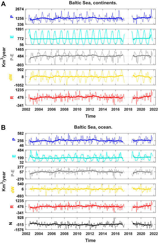
FIGURE 2. WT time series in the Baltic Sea (Kattegat and Skagerrak straits are excluded) for both (A) continental drainage basins and (B) ocean basins. Thick lines depict the 12-month moving average. Negative (positive) values of N correspond to Baltic Sea outflows (inflow). The labels in the y-axis of each time series correspond to their mean, maximum, and minimum values.

Mean Values of WT

The mean values of all WT components of the Baltic Sea are shown in Table 3. The continental drainage basins receive net precipitation of 484 ± 20 km³/year, which produces R = 476 ± 17 km³/year (Table 1). This estimate of R agrees with the average of reported values of river runoff (Table 1). P also exceeds E in the sea, producing a net inflow of P−E = 57 ± 7 km³/year, in contrast with the global ocean or the Mediterranean-Black Sea system where E exceeds P (Hartmann, 1994; García-García et al., 2020; García-García et al., 2022). Then, the excess fresh water given by P−E + R leaves the Baltic Sea through the Arkona Sea at a mean rate of 515 ± 27 km³/year. Surprisingly, this value is identical, within error estimates, to the average net outflow, 508 ± 23 km³/year, estimated from previously reported values (Table 2), despite the differences in the targeted period of study, methodology, and data used. The net WT component N is the result of a stratified water exchange in both senses. Saltier water from the Atlantic Ocean enters the Baltic Sea near the bottom at a mean rate of 1,301 ± 227 km³/year, while less salty water leaves the Baltic Sea near the surface at a mean rate of 1,793 ± 214 km³/year.

TABLE 3

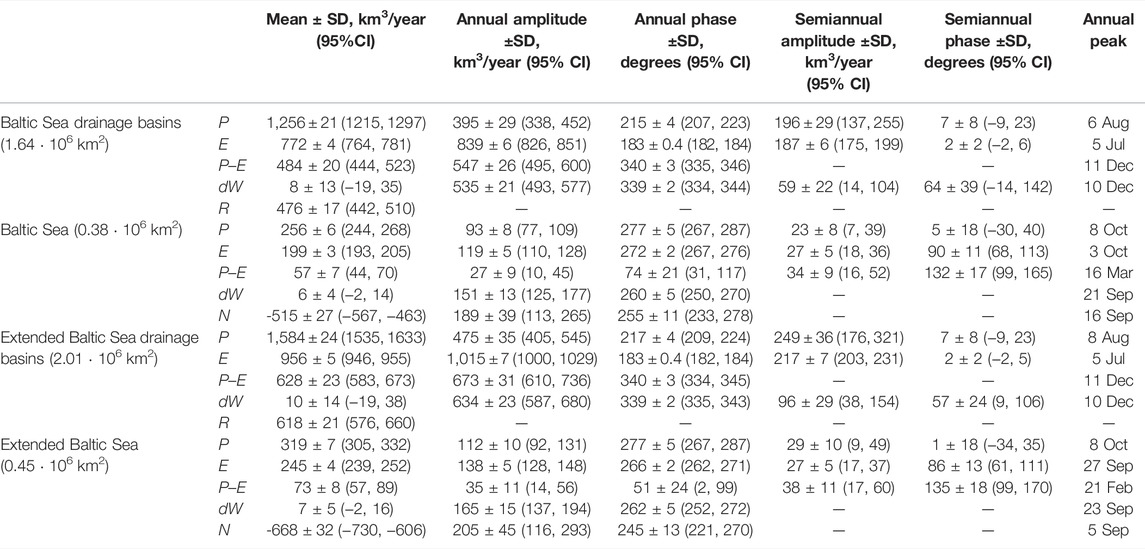
TABLE 3. Mean, annual, and semiannual signal, estimated from Eq. 2, for WT components for both the Baltic Sea and the extended Baltic Sea (Kattegat and Skagerrak straits are included) shown in Figure 2 and Supplementary Figure S1. Time spans from 06/2002–06/2017 to 06/2018–11/2021. Units are km³/year for mean values and amplitudes, and degrees for phases. In each cell the following are reported: 1) the point estimate (based on the original time series) plus/minus the standard deviation (SD; estimated by bootstrap based on the reduced series, that is from 181 observations); 2) the 95% confidence interval, CI, computed as the point estimate plus/minus 2 SD. Empty cells correspond to the amplitude of a phase of periodic (annual/semiannual) components not statistically significant at the significance level α = 0.05. Regional surface areas are estimated with our grid resolution (see Figure 1). Negative N means a flux from the Baltic Sea to the North Sea. For the conversion of mass transport to volume transport, water density is fixed to 1,000 kg/m³ for fresh water and 1,025 kg/m³ for seawater.

When the region is extended to include the Kattegat and Skagerrak straits, the drainage basin increases from 1.64 · 10⁶ km² to 2.01 · 10⁶ km², and the oceanic surface area increases from 0.38 · 10⁶ km² to 0.45 · 10⁶ km². On land, the net precipitation increases to P−E = 628 ± 23 km³/year, and the drainage to the sea increases to R = 618 ± 21 km³/year (Table 3). In the ocean, net precipitation is 73 ± 8 km³/year, which together with the contribution of R yields a net outflow to the North Sea of 668 ± 32 km³/year. A schematic representation of the averaged water cycle of the Baltic Sea and that of the extended Baltic Sea are shown in Figure 3.

FIGURE 3

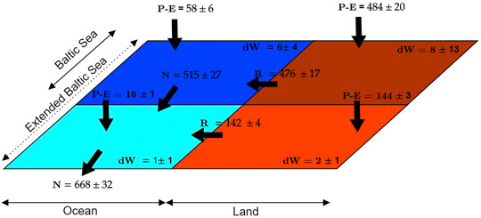
FIGURE 3. Mean WT components that make up the water cycle in the extended Baltic Sea (Kattegat and Skagerrak straits are included). Units are km³/year and errors are the standard deviation of the mean estimated by stationary bootstrap based on the reduced series (with 181 observations).

Seasonal Signal of WT

The Baltic Sea (either including the Kattegat and Skagerrak straits or not) receives an excess of fresh water that must leave the basin. However, the water mass imbalance is not compensated instantaneously, and a climatological signal arises in all WT components and water mass budgets. To analyze such climatology, the annual cycle of each WT component is estimated by averaging the signal of all Januarys, all Februarys, and so on. Figure 4 shows the average year or climatology for all WT components displayed in Figure 2.

FIGURE 4

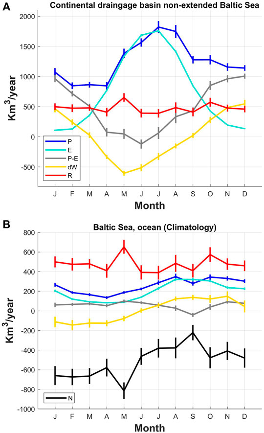
FIGURE 4. Climatology (monthly averages) of signals shown in Figure 2.

In the continental drainage region of the Baltic Sea, both P and E climatologies show a good agreement in spring and summer, with maximum values of 1,822 ± 99 km³/year and 1,759 ± 18 km³/year occurring in July for P and E, respectively (Figure 4A). In autumn and winter, E is reduced much more than P, reaching a minimum of 109 ± 10 km³/year in December and January. This disagreement during the cold season is probably due to the increase of snow percentage in P, which is harder to evaporate than liquid water. This result agrees with the annual cycle of dW, which mimics the P−E climatology, showing a Pearson correlation of 0.81 ± 0.02 between the original time series (Figure 5A). Positive (negative) values of dW represent an increase (decrease) in the water budget. In particular, dW shows a mean value of 340 ± 80 km³/year for autumn and winter, when snow accumulation (and low E) is expected, and −317 ± 95 km³/year for spring and summer, when ice melting (and E) takes place. dW and E are strongly anticorrelated, showing a correlation coefficient of −0.76 ± 0.02 between their original time series. The annual maximum and minimum of dW are reached in December (547 ± 66 km³/year) and May (−605 ± 40 km³/year), respectively. This minimum is produced by the annual maximum of R = 654 ± 71 km³/year, although there is no significant correlation between dW and R.

FIGURE 5

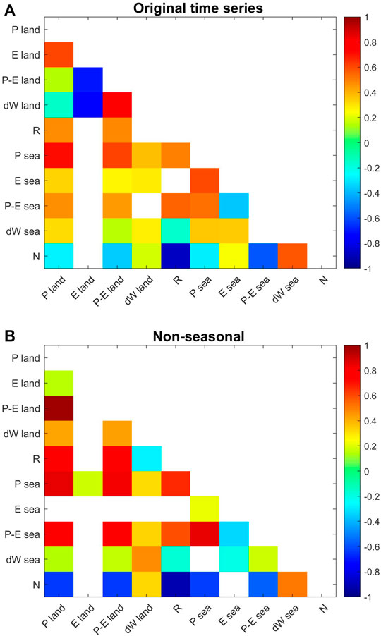
FIGURE 5. Pearson correlation coefficients between (A) all seasonal signals shown in Figure 2 and (B) all nonseasonal signals shown in Figure 7.

In the Baltic Sea, the annual cycle of dW mimics that of P and E, despite Pearson correlations between the original time series being 0.36 ± 0.05 and 0.35 ± 0.045, respectively. Hereafter, when SD is given with more than two decimals, it is used to reconstruct the 95% CI as plus/minus 2 SD if needed. Both dW and P present maximum values from August to November and minimum from February to April (Figure 4B). The annual maximum of E is reached between August and October, while the annual minimum takes place between February and May, when sea-ice coverage is maximum (Omstedt et al., 1997; Vihma and Haapala, 2009). The larger values of dW found during the second half of the year represent an increase in the water budget, which is related to a minimum net outflow N = 390 ± 42 km³/year from July to December. From January to May, N is almost doubled up to 678 ± 38 km³/year. Except for this half-year difference, N mirrors the month-to-month variability of R, presenting a significant Pearson correlation between the original time series of −0.88 ± 0.015 (Figure 6A), reminding that negative values of N represent the Baltic outflow. Then the greater the R, the larger (in absolute value) the N, that is, the larger the output. As shown in Figure 4B, the annual maximum of R (654 ± 71 km³/year) is reached in May, which results in the annual maximum magnitude of N (814 ± 85 km³/year).

FIGURE 6

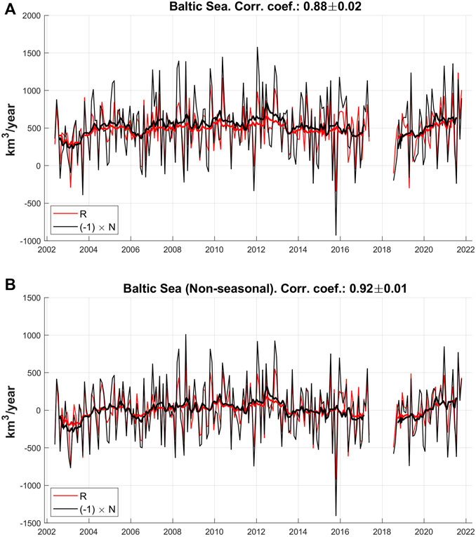
FIGURE 6. (A) Seasonal and (B) nonseasonal water transport from land to the Baltic Sea (red curve) and net outflow from the Baltic Sea (black curve). Black curve represents −N. As N is multiplied by −1, positive (negative) values of black curve represent above-average (below-average) flows. Correlations between R and N are negative in both cases.

The seasonal signals of WT components, of both continental and oceanic regions, in the extended Baltic Sea are almost identical to those of the (non-extended) Baltic Sea, although with larger absolute values for P, E, R, and N (Supplementary Figure S2).

Nonseasonal Signal of WT

The nonseasonal signal is obtained by subtracting the climatology from the original signal. This way is more appropriate than fitting an annual sinusoid since the average year is not always sinusoidal in shape (Figure 4). In general, all components show a larger nonseasonal variability on land than in the ocean (Figure 7). All components present a nonsignificant linear trend.

FIGURE 7

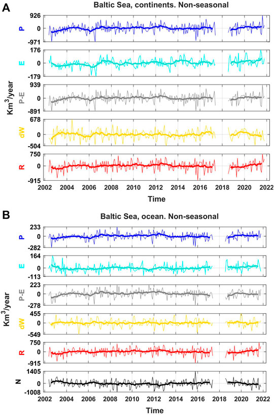
FIGURE 7. Nonseasonal signal of WT components shown in Figure 2. The labels in the y-axis of each time series correspond to their mean, maximum, and minimum values.

On land, the nonseasonal variability of P is the largest one, and it is propagated to P–E, dW, and R. Pearson correlation coefficients between P and P–E, R, and dW are 0.98 ± 0.0025, 0.74 ± 0.035, and 0.42 ± 0.06, respectively (Figure 5B). Note that 1) the correlation between the original time series of P and P–E was very low (0.15 ± 0.05), but there is a high correlation of 0.98 ± 0.003 between the nonseasonal time series; 2) the correlation between the original time series of P–E and E is –0.70 ± 0.025, but it is not statistically significant between the nonseasonal time series. This means that P–E on land is driven by E at a seasonal scale and by P at a non-seasonal one. In the Baltic Sea, P and P–E show a high correlation (0.85 ± 0.025) for the nonseasonal signals and a lower one for the original signals (0.53 ± 0.05). On the contrary, E and P–E show a similar correlation around –0.35 ± 0.065 for both seasonal and nonseasonal signals. Then, P has more influence than E on P–E variability at both seasonal and nonseasonal scales. It is also significant that the P signal is similar over both continents and ocean (the corresponding correlation coefficient is 0.86 ± 0.025), unlike E, for which no significant correlation is found between the continental and oceanic signals.

The interannual variability of P, P–E, and R is quite strong, showing differences of around 200–250 km³/year between some annual averages. Such differences even reach values around 470 km³/year for N. For example, in 2012, both P and P–E showed an above-average annual mean value of 1,406 km³/year and 643 km³/year, respectively, which produced a maximum R = 658 km³/year. On the contrary, in 2006, a below-average P = 1,159 km³/year produced a below-average P–E = 444 km³/year, which in turn produced a below-average R = 395 km³/year. Although P–E was 40 km³/year lower than average during this year, R decreased double that amount, 81 km³/year, because there was an extra accumulation of water in the continents of 41 km³/year. On the other hand, the correlation between R and N increases in magnitude from –0.88 ± 0.015 (original series in Figure 2) to –0.92 ± 0.01 for the nonseasonal signals (Figure 6). This means that the water transported by R into the Baltic Sea produces almost simultaneously, or with a lag of less than a month, an outflow from the Baltic Sea. The above-average R in 2012 produced an above-average outflow of water mass from the Baltic Sea of 833 km³/year, while the below-average R in 2006 reduced N to more than half until 360 km³/year. The reduction of N is larger than that of R because P–E over the Baltic Sea also showed an above-average annual mean in 2012 (110 km³/year) and a below-average in 2006 (53 km³/year) that increased and reduced N, respectively.

Although the climatology of N shows an outflow from the Baltic Sea every month of the year, it can sporadically reverse. For example, in October 2015, the net WT was N = 927 km³/year (1,400 km³/year more than the average value in October), which represented a huge net inflow to the Baltic Sea from the Atlantic Ocean that doubled the mean outflow of the 2002–2021 period. This event was produced by extremely low values of R and unusual high net evaporation over the Baltic Sea (Figures 6, 7), that is, by a decrease of freshwater input. On the other hand, a positive value of dW indicates an increment of the water mass budget in the Baltic Sea, which should have been produced by a Major Baltic Inflow (MBI). The MBI plays an important role in the Baltic Sea conditions because it introduces large volumes of saline and oxygen-rich water into the bottom layers that partially determine the faunal and floral composition. These three events (low R, high net E, and MBI) agree with the fact that the lower the runoff, the larger the deep-water salinity (Hänninen et al., 2000). However, note that N is not a direct estimate of MBI since some water transport models suggest that an increase in the outflow in the uppermost layer is related to an increase in the inflow in the bottom layer (Lehman and Hinrichsen, 2002). Mohrholz et al. (2015) reported a very strong MBI produced by wind anomalies in December 2014. In that month, N showed 523 km³/year more than the average value found for all Decembers, which is a third of the anomaly reported in October 2015. However, the MBI of December 2014 was stronger than that of October 2015 (Mohrholz, 2018).

The extended Baltic Sea shows the same kind of nonseasonal variability (Supplementary Figure S3) and the relationship between the WT components (Supplementary Figures S4, S5) above shown for the Baltic Sea.

Influence of NAO on WT

The NAO is a climate atmospheric index that summarizes the surface pressure variability over the North Atlantic. It can be estimated as the sea level air pressure differences between the high-pressure system located over the Azores islands and the low-pressure system over Iceland. Then, changes in the NAO are associated with changes in the westerly winds in the North Atlantic, which influence weather conditions in Europe and eastern North America. In particular, NAO effects are stronger in winter, when positive (negative) phases of NAO produce above-average (below-average) P and temperature in northern Europe, and below-average (above-average) P and temperature in the Mediterranean region and Hudson Bay area (Hurrell, 1995; Hurrell et al., 2003). In the Baltic Sea, positive (negative) winter NAO decreases (increases) the sea-ice extent (Omstedt and Chen, 2001; Heino et al., 2008), and rises (drops) the sea level (Andersson, 2002). We explore the influence of winter NAO on WT components of the Baltic Sea region as follows. The NAO index estimated by NOAA (https://www.cpc.ncep.noaa.gov/products/precip/CWlink/pna/nao.shtml; data accessed on 26/01/2022) and the nonseasonal time series shown in Figure 7 are averaged over winter months (December to March), and their Pearson correlation coefficients are estimated. Only 5 out of the 10 WT components present a statistically significant correlation: 0.64 ± 0.09 for continental P, 0.78 ± 0.05 for continental E, 0.52 ± 0.12 for continental P–E, 0.39 ± 0.16 for oceanic P, and 0.55 ± 0.12 for oceanic P–E. We have not found a significant correlation between NAO and R for the period 2002–2021, but it does not mean that it does not exist for a different period. For example, Johansson (2016) found a correlation of 0.47 between NAO and runoff for the period 1990–2009, but not for the period 1960–1979.

Discussion

Assuming the water budget equation, we used an atmospheric reanalysis and satellite-based time-variable gravity data to estimate the hydrological cycle of the Baltic Sea and its continental catchment region for the period 2002–2021. We provide the annual mean, climatology, and nonseasonal signals for all WT components. In general, the mean hydrological cycle and the climatology of P−E are similar to those reported by Jacob (2001) from a global and a regional climate model.

We have estimated a freshwater input from the continent, including superficial runoff (in river courses or not) and underground water discharge, of R = 476 ± 17 km³/year. Our results about the climatology of R share some important features with previous studies based on almost a century of data and reconstructed data. In agreement with the existing literature (Cyberski and Wróblewski, 2000; Meier and Kauker, 2003), we found an annual maximum in May. There are, however, some important differences. In particular, in comparison with previous studies of the climatology of R, we found: 1) a lower annual range (264 km³/year versus ∼ 480 km³/year); 2) a larger increase from September to the local maxima in October (164 km³/year versus 12 km³/year); and 3) a lower annual maximum (654 km³/year versus 728 km³/year). These differences may be a consequence of a real change in the climatology but also of the different periods and methodology used. At the interannual scale, we have reported values of R = 395 km³/year in 2006 and R = 658 km³/year in 2012. This type of variability has been observed in previous studies. For example, Winsor et al. (2001) reported an annual mean river runoff of ∼ 330 km³/year in 1976 and ∼ 535 km³/year in 1981 (see also Meier and Kauker, 2003).

Another key result of this study is the estimated net water mass exchange between the Baltic Sea and the Atlantic Ocean. We report a mean net outflow of 515 ± 27 km³/year that evacuates the surplus of fresh water in the Baltic Sea, whose 92% comes from R. In addition, N shows a clear annual cycle with an amplitude of 189 ± 39 km³/year that peaks around September 16. On average, all months present a net outflow from the Baltic Sea, although in particular months, N flows in the opposite direction. On top of the climatology, N shows a significant interannual variability mainly driven by R. It is worth noting that such interannual variability is observed in both surface outflow and near-bottom inflow (Lehmann and Hinrichsen, 2002).

Conclusion

During the last 2 decades, knowledge of the dynamics of the Earth system has undergone a tremendous advance, thanks to the GRACE missions, whose data have become key for many new applications aimed to enhance our knowledge in relevant problems. In this study, we illustrate the fundamental role of GRACE data for the study of the net seawater mass exchange in the Baltic Sea (and the hydrological cycle in the region) using an algorithm proposed by García-García et al. (2020). When the exchange of water can only take place along one path, as is the case with semi-enclosed basins like the Baltic Sea, the algorithm provides net WT through that path. Using GRACE and ERA5 data as inputs, we have estimated the mean values, the climatology, and the interannual variability of the water exchange between the Baltic Sea and the open ocean, and also for an extended region including the Kattegat and Skagerrak straits. In this case, the mean net outflow from the extended Baltic Sea to the North Sea is 668 ± 32 km³/year, which is 30% larger than the net outflow from the non-extended Baltic Sea. This increment is produced by a continental contribution of 618 ± 21 km³/year, which is also an increase of 30% with respect to the non-extended Baltic Sea. In the annual amplitude, a smaller increment of 8% is observed, although it is not statistically significant. The overall conclusion is that the difference in water transport between the extended and non-extended regions considered in this study is mainly produced by the mean value.

The strengths of the methodology presented in this study are the following:

1) The results are independent of those reported in previous studies, which were mostly based on in situ observations and models.

2) The studied regions can be easily redefined, which makes possible the estimation of net water fluxes at any passage or section. This can be useful to make comparisons with independent studies or to define boundary conditions for oceanic models.

3) The results are based on two datasets (GRACE/GRACE-FO and ERA5) which are expected to be updated periodically. Therefore, the proposed methodology is a potential tool for continuously monitoring the hydrological cycle of the Baltic Sea, as well as to understand its time evolution. In this respect, when longer time series will be available, the proposed methodology would allow to detect the predicted changes consequence of the ongoing climate change.

Data Availability Statement

Publicly available datasets were analyzed in this study. These data can be found at: https://cds.climate.copernicus.eu/cdsapp#!/home http://www2.csr.utexas.edu/grace https://www.cpc.ncep.noaa.gov/products/precip/CWlink/pna/nao.shtml.

Author Contributions

DG-G designed the study. AB processed datasets and wrote the first draft of the manuscript. MT and MV implemented the bootstrap and contributed to other aspects of the data analysis. MV also provided funding for the research. All authors discussed and interpreted the results and contributed to the writing and revision of the manuscript.

Funding

DG-G, MV, and MT are partially funded by the Spanish Ministry of Science, Innovation, and Universities grant number RTI2018-093874-B-100, and the Generalitat Valenciana grant number GVA-THINKINAZUL/2021/035. DG-G and MV are partially funded by the Generalitat Valenciana grant number PROMETEO/2021/030. J-MS thanks the joint funding received from Generalitat Valenciana and the European Social Fund under Grant APOSTD/2020/254. AB benefits from a doctoral study allowance financed by the Algerian Ministry of Higher Education and Scientific Research.

Conflict of Interest

The authors declare that the research was conducted in the absence of any commercial or financial relationships that could be construed as a potential conflict of interest.

Publisher’s Note

All claims expressed in this article are solely those of the authors and do not necessarily represent those of their affiliated organizations, or those of the publisher, the editors, and the reviewers. Any product that may be evaluated in this article, or claim that may be made by its manufacturer, is not guaranteed or endorsed by the publisher.

Acknowledgments

All data used in this study are publicly available, and we thank all the organizations that provided them: ERA5 data provided by the Copernicus Climate Change Service Climate Data Store (CDS), https://cds.climate.copernicus.eu/cdsapp#!/home; GRACE time-variable gravity data provided by CSR, University of Texas, http://www2.csr.utexas.edu/grace; and North Atlantic Oscillation (NAO) from NOAA Climate Prediction Center (CPC).

Supplementary Material

The Supplementary Material for this article can be found online at: https://www.frontiersin.org/articles/10.3389/feart.2022.879148/full#supplementary-material

References

Andersson, H. C. (2002). Influence of Long-Term Regional and Large-Scale Atmospheric Circulation on the Baltic Sea Level. Tellus A: Dynamic Meteorology Oceanography 54 (1), 76–88. doi:10.3402/tellusa.v54i1.12125

CrossRef Full Text | Google Scholar

Bergström, S., and Carlsson, B. (1994). River Runoff to the Baltic Sea: 1950-1990. Ambio. R. Swedish Acad. Sci. 23 (4/5), 280–287.

Google Scholar

Chao, B. F. (2016). Caveats on the Equivalent Water Thickness and Surface Mascon Solutions Derived from the GRACE Satellite-Observed Time-Variable Gravity. J. Geod 90, 807–813. doi:10.1007/s00190-016-0912-y

CrossRef Full Text | Google Scholar

Chao, B. F. (2005). On Inversion for Mass Distribution from Global (Time-variable) Gravity Field. J. Geodynamics 39, 223–230. doi:10.1016/j.jog.2004.11.001

CrossRef Full Text | Google Scholar

Chen, J., Tapley, B., Seo, K. W., Wilson, C., and Ries, J. (2019). Improved Quantification of Global Mean Ocean Mass Change Using GRACE Satellite Gravimetry Measurements. Geophys. Res. Lett. 46, 13984–13991. doi:10.1029/2019GL085519

CrossRef Full Text | Google Scholar

Cyberski, J., and Wróblewski, A. (2000). Riverine Water Inflows and the Baltic Sea Water Volume 1901–1990. Hydrol. Earth Syst. Sci. 4, 1–11. doi:10.5194/hess-4-1-2000

CrossRef Full Text | Google Scholar

Dargahi, B., and Cvetkovic, V. (2017). Tracer Transport and Exchange Processes in the Baltic Sea 2000-2009. J. Oceanogr Mar. Res. 5, 156. doi:10.4172/2572-3103.1000156

CrossRef Full Text | Google Scholar

Dargahi, B., Kolluru, V., and Cvetkovic, V. (2017). Multi-layered Stratification in the Baltic Sea: Insight from a Modeling Study with Reference to Environmental Conditions. Jmse 5, 1–2. doi:10.3390/jmse5010002

CrossRef Full Text | Google Scholar

Durack, P. J., Wijffels, S. E., and Matear, R. J. (2012). Ocean Salinities Reveal Strong Global Water Cycle Intensification during 1950 to 2000. Science 336, 6080455–6080458. doi:10.1126/science.1212222

PubMed Abstract | CrossRef Full Text | Google Scholar

Ellmann, A. (2004). Effect of the GRACE Satellite mission on Gravity Field Studies in Fennoscandia and the Baltic Sea Region. Proc. Estonian Acad. Sci. Geology. 53 (2), 67–93. doi:10.3176/geol.2004.2.01

CrossRef Full Text | Google Scholar

Eom, J., Seo, K.-W., and Ryu, D. (2017). Estimation of Amazon River Discharge Based on EOF Analysis of GRACE Gravity Data. Remote Sensing Environ. 191, 55–66. doi:10.1016/j.rse.2017.01.011

CrossRef Full Text | Google Scholar

Fatolazadeh, F., and Goïta, K. (2021). Mapping Terrestrial Water Storage Changes in Canada Using GRACE and GRACE-FO. Sci. Total Environ. 779, 146435. doi:10.1016/j.scitotenv.2021.146435

PubMed Abstract | CrossRef Full Text | Google Scholar

García-García, D., Vigo, M.I., Trottini, M., Vargas, J., and Sayol, J.M. (2022). Hydrological cycle of the Mediterranean-Black Sea system. Climate Dynamics, 1–20. doi:10.1007/s00382-022-06188-2

CrossRef Full Text | Google Scholar

García-García, D., Vigo, M.I., and Trottini, M. (2020). Water transport among the world’s ocean basins within the water cycle. Earth Syst. Dynam. 11, 1089–1106. doi:10.5194/esd-11-1089-2020

CrossRef Full Text | Google Scholar

Giorgi, F. (2006). Climate change hot-spots. Geophys. Res. Lett. 33, 8. doi:10.1029/2006GL025734

CrossRef Full Text | Google Scholar

Greve, P., Orlowsky, B., Mueller, B., Sheffield, J., Reichstein, M., and Seneviratne, S. I. (2014). Global Assessment of Trends in Wetting and Drying over Land. Nat. Geosci 7, 716–721. doi:10.1038/ngeo2247

CrossRef Full Text | Google Scholar

Gustafsson, B. (1997). Interaction between the Baltic Sea and the North Sea. Deutsche Hydrographische Z. 49, 165–183. doi:10.1007/bf02764031

CrossRef Full Text | Google Scholar

Håkanson, L., and Lindgren, D. (2010). Water Transport and Water Retention in Five Connected Subbasins in the Baltic Sea-Simulations Using a General Mass-Balance Modeling Approach for Salt and Substances. J. Coastal Res. 262 (2), 241–264. doi:10.2112/08-1082.1

CrossRef Full Text | Google Scholar

Hänninen, J., Mäkinen, K., Rajasilta, M., and Vuorinen, I. (2021). The Baltic Sea and the Adjacent North Sea Silicate Concentrations. Estuarine, Coastal Shelf Sci. 249, 107110. doi:10.1016/j.ecss.2020.107110

CrossRef Full Text | Google Scholar

Hänninen, J., Vuorinen, I., and Hjelt, P. (2000). Climatic Factors in the Atlantic Control the Oceanographic and Ecological Changes in the Baltic Sea. Limnol. Oceanogr. 45 (3), 703–710. doi:10.4319/lo.2000.45.3.0703

CrossRef Full Text | Google Scholar

Hänninen, J., and Vuorinen, I. (2011). Time-Varying Parameter Analysis of the Baltic Sea Freshwater Runoffs. Environ. Model. Assess. 16 (1), 53–60. doi:10.1007/s10666-010-9231-5

CrossRef Full Text | Google Scholar

Hansson, D., Eriksson, C., Omstedt, A., and Chen, D. (2011). Reconstruction of River Runoff to the Baltic Sea, AD 1500-1995. Int. J. Climatol. 31 (5), 696–703. doi:10.1002/joc.2097

CrossRef Full Text | Google Scholar

Hartmann, D. L. (1994). Global Physical Climatology. Amsterdam, the Netherlands: Elsevier.

Google Scholar

Heino, R., Tuomenvirta, H., Vuglinsky, V. S., and Gustafsson, B. G. (2008). “Past and Current Climate Change,” in The BACC Author Team Assessment of Climate Change for the Baltic Sea Basin (Berlin-Heidelberg: Springer-Verlag), 72. doi:10.1007/978-3-540-72786-6_2

CrossRef Full Text | Google Scholar

Held, I. M., and Soden, B. J. (2006). Robust Responses of the Hydrological Cycle to Global Warming. J. Clim. 19 (21), 5686–5699. doi:10.1175/jcli3990.1

CrossRef Full Text | Google Scholar

Hersbach, H., de Rosnay, P., Bell, B., Schepers, D., Simmons, A., Soci, C., et al. (2018). Operational Global Re- Analysis: Progress, Future Directions, and Synergies with NWP. ERA Report Series 27. Shinfield Park, Reading, Berkshire, England: European Centre for Medium Range Weather Forecasts.

Google Scholar

Huntington, T. G. (2006). Evidence for Intensification of the Global Water Cycle: Review and Synthesis. J. Hydrol. 319 (1-4), 83–95. doi:10.1016/j.jhydrol.2005.07.003

CrossRef Full Text | Google Scholar

Hurrell, J. W. (1995). Decadal Trends in the North Atlantic Oscillation: Regional Temperatures and Precipitation. Science 269 (5224), 676–679. doi:10.1126/science.269.5224.676

PubMed Abstract | CrossRef Full Text | Google Scholar

Hurrell, J. W., Kushnir, Y., Ottersen, G., and Visbeck, M. (2003). An Overview of the North Atlantic Oscillation. Washington: Washington American Geophysical Union Vol. 134, 1–35. doi:10.1029/134GM01

CrossRef Full Text | Google Scholar

Jacob, D. (2001). A Note to the Simulation of the Annual and Inter-annual Variability of the Water Budget over the Baltic Sea Drainage basin. Meteorology Atmos. Phys. 77 (1), 61–73. doi:10.1007/s007030170017

CrossRef Full Text | Google Scholar

Jin, S., and Feng, G. (2013). Large-scale Variations of Global Groundwater from Satellite Gravimetry and Hydrological Models, 2002-2012. Glob. Planet. Change 106, 20–30. doi:10.1016/j.gloplacha.2013.02.008

CrossRef Full Text | Google Scholar

Johansson, J. (2016). Total and Regional Runoff to the Baltic Sea. Baltic Sea Environment Fact Sheet. Available at: http://www.helcom.fi/baltic-sea-trends/environment-fact-sheets/ (Accessed February 2022).

Google Scholar

Jordà, G., Von Schuckmann, K., Josey, S. A., Caniaux, G., García-Lafuente, J., Sammartino, S., et al. (2017). The Mediterranean Sea Heat and Mass Budgets: Estimates, Uncertainties and Perspectives. Prog. Oceanogr. 156, 174–208. doi:10.1016/j.pocean.2017.07.001

CrossRef Full Text | Google Scholar

Lee, E., Livino, A., Han, S.-C., Zhang, K., Briscoe, J., Kelman, J., et al. (2018). Land Cover Change Explains the Increasing Discharge of the Paraná River. Reg. Environ. Change 18 (6), 1871–1881. doi:10.1007/s10113-018-1321-y

PubMed Abstract | CrossRef Full Text | Google Scholar

Lehmann, A., and Hinrichsen, H. H. (2002). Water, Heat, and Salt Exchange between the Deep Basins of the Baltic Sea. Boreal Environ. Res. 7 (4), 405–415.

Google Scholar

Li, Q., Zhong, B., Luo, Z., and Yao, C. (2016). GRACE-based Estimates of Water Discharge over the Yellow River basin. Geodesy. Geodynamics 7 (3), 187–193. doi:10.1016/j.geog.2016.04.007

CrossRef Full Text | Google Scholar

Lorenz, C., Kunstmann, H., Devaraju, B., Tourian, M. J., Sneeuw, N., and Riegger, J. (2014). Large-Scale Runoff from Landmasses: A Global Assessment of the Closure of the Hydrological and Atmospheric Water Balances*. J. Hydrometeorology 15 (6), 2111–2139. doi:10.1175/JHM-D-13-0157.s1

CrossRef Full Text | Google Scholar

Markonis, Y., Papalexiou, S. M., Martinkova, M., and Hanel, M. (2019). Assessment of Water Cycle Intensification over Land Using a Multisource Global Gridded Precipitation Dataset. J. Geophys. Res. Atmos. 124 (21), 11175–11187. doi:10.1029/2019JD030855

CrossRef Full Text | Google Scholar

Matthäus, W., and Schinke, H. (1999). The Influence of River Runoff on Deep Water Conditions of the Baltic Sea. Hydrobiologia. Biological, Phys. Geochemical Features Enclosed Semi-enclosed Mar. Syst. 393, 1–10.

Google Scholar

Meier, H. E. M., and Döscher, R. (2002). Simulated Water and Heat Cycles of the Baltic Sea Using a 3D Coupled Atmosphere – Ice – Ocean Model. Boreal Environ. Res. 7, 327–334.

Google Scholar

Meier, H. E. M., and Kauker, F. (2003). Modeling Decadal Variability of the Baltic Sea: 2. Role of Freshwater Inflow and Large-Scale Atmospheric Circulation for Salinity. J. Geophys 108, 1–10. doi:10.1029/2003jc001799

CrossRef Full Text | Google Scholar

Mikulski, Z. (1986). Water balance of the Baltic Sea. Geophysica 17120 (1–2), 159.

Google Scholar

Mohrholz, V. (2018). Major Baltic inflow statistics - Revised. Front. Mar. Sci. 5. doi:10.3389/fmars.2018.00384

CrossRef Full Text | Google Scholar

Mohrholz, V., Naumann, M., Nausch, G., Krüger, S., and Gräwe, U. (2015). Fresh oxygen for the Baltic Sea - an exceptional saline inflow after a decade of stagnation. J. Marine Sys. 148, 152–166. doi:10.1016/j.jmarsys.2015.03.005

CrossRef Full Text | Google Scholar

Oki, T., and Sud, Y. C. (1998). Design of Total Runoff Integrating Pathways (TRIP)-A Global River Channel Network. Earth Interact. 2, 1–37. doi:10.1175/1087-3562(1998)002<0001:dotrip>2.3.co;2

CrossRef Full Text | Google Scholar

Omstedt, A., and Chen, D. (2001). Influence of atmospheric circulation on the maximum ice extent in the Baltic Sea. J. Geophys. Res. 106, 4493–4500. doi:10.1029/1999jc000173

CrossRef Full Text | Google Scholar

Omstedt, A., Elken, J., Lehmann, A., and Piechura, J. (2004). Knowledge of the Baltic Sea physics gained during the BALTEX and related programs. Progress Oceanography 63, 1–28. doi:10.1016/j.pocean.2004.09.001

CrossRef Full Text | Google Scholar

Omstedt, A., Meuller, L., and Nyberg, L. (1997). Interannual, seasonal, and regional variations of precipitation and evaporation over the Baltic Sea. Ambio 26 (8), 484–492.

Google Scholar

Omstedt, A., and Nohr, C. (2004). Calculating the water and heat balances of the Baltic Sea using ocean modeling and available meteorological, hydrological, and ocean data. Tellus A: Dynamic Meteorology and Oceanography 56 (4), 400–414. doi:10.3402/tellusa.v56i4.14428

CrossRef Full Text | Google Scholar

Omstedt, A., and Rutgersson, A. (2000). Closing the Water and Heat Cycles of the Baltic Sea. metz 9 (1), 59–66. doi:10.1127/metz/9/2000/59

CrossRef Full Text | Google Scholar

Pajak, K., and Birylo, M. (2017). Seasonal Baltic Sea Level Changes in Coastal Zone. Eur. Water 59, 185–192.

Google Scholar

Patton, A., Politis, D. N., and White, H. (2009). Correction to “Automatic Block-Length Selection for the Dependent Bootstrap”. Economet. Rev. 28, 372–375. doi:10.1080/07474930802459016

CrossRef Full Text | Google Scholar

Peltier, W. R., Argus, D. F., and Drummond, R. (2018). Comment on “An Assessment of the ICE-6GC (VM5a) Glacial Isostatic Adjustment Model” by Purcell et al. J. Geophys. Res.-Solid 123, 2019–2028. doi:10.1002/2016JB013844

CrossRef Full Text | Google Scholar

Placke, M., Meier, H. E. M., Gräwe, U., Neumann, T., Frauen, C., and Liu, Y. (2018). Long-term Mean Circulation of the Baltic Sea as Represented by Various Ocean Circulation Models. Front. Mar. Sci. 5, 287. doi:10.3389/fmars.2018.00287

CrossRef Full Text | Google Scholar

Politis, D. N., and Romano, J. P. (1994). The Stationary Bootstrap. J. Am. Stat. Assoc. 89, 1303–1313. doi:10.1080/01621459.1994.10476870

CrossRef Full Text | Google Scholar

Save, H. (2019). CSR GRACE RL06 Mascon Solutions, Texas Data Repository Dataverse. doi:10.18738/T8/UN91VR

CrossRef Full Text | Google Scholar

Save, H., Bettadpur, S., and Tapley, B. D. (2016). High Resolution CSR GRACE RL05 Mascons. J. Geophys. Res.-Solid 121, 7547–7569. doi:10.1002/2016JB013007

CrossRef Full Text | Google Scholar

Stramska, M., and Aniskiewicz, P. (2019). Satellite Remote Sensing Signatures of the Major Baltic Inflows. Remote Sensing 11, 954. doi:10.3390/rs11080954

CrossRef Full Text | Google Scholar

Sun, Y., Riva, R., and Ditmar, P. (2016). Optimizing Estimates of Annual Variations and Trends in Geocenter Motion and J2 From a Combination of GRACE Data and Geophysical Models. J. Geophys. Res. Solid Earth 121. doi:10.1002/2016JB013073

CrossRef Full Text | Google Scholar

Swenson, S., Chambers, D., and Wahr, J. (2008). Estimating Geo- Center Variations From a Combination of GRACE and Ocean Model Output. J. Geophys. Res. 113, B08410. doi:10.1029/2007JB005338

CrossRef Full Text | Google Scholar

Syed, T. H., Famiglietti, J. S., and Chambers, D. P. (2009). GRACE-based Estimates of Terrestrial Freshwater Discharge from basin to continental Scales. J. Hydrometeorology 10 (1), 22–40. doi:10.1175/2008JHM993.1

CrossRef Full Text | Google Scholar

Syed, T. H., Famiglietti, J. S., Chen, J., Rodell, M., Seneviratne, S. I., Viterbo, P., et al. (2005). Total basin Discharge for the Amazon and Mississippi River Basins from GRACE and a Land-Atmosphere Water Balance. Geophys. Res. Lett. 32 (24), 1–5. doi:10.1029/2005GL024851

CrossRef Full Text | Google Scholar

The BACC Author Team (2008). Assessment of Climate Change for the Baltic Sea basin. Berlin: Springer Science & Business Media. doi:10.1007/978-3-540-72786-6

CrossRef Full Text | Google Scholar

Vihma, T., and Haapala, J. (2009). Assessment of Climate Change for the Baltic Sea Basin. Prog. Oceanography 80 (3–4), 129–148. doi:10.1016/j.pocean.2009.02.002

CrossRef Full Text | Google Scholar

Virtanen, J., Mäkinen, J., Bilker-Koivula, M., Virtanen, H., Nordman, M., Kangas, A., et al. (2010). Baltic Sea Mass Variations from GRACE: Comparison with In Situ and Modelled Sea Level Heights. Gravity. Geoid. Earth Observation 135, 571–577. doi:10.1007/978-3-642-10634-7_76

CrossRef Full Text | Google Scholar

Wahr, J., Molenaar, M., and Bryan, F. (1998). Time Variability of the Earth’s Gravity Field: Hydrological and Oceanic Effects and Their Possible Detection Using GRACE. J. Geophys. Res. 103 (30), 229. doi:10.1029/98jb02844

CrossRef Full Text | Google Scholar

Winsor, P., Rodhe, J., and Omstedt, A. (2001). The Baltic Sea Ocean Climate: an Analysis of 100 Yr of Hydrographic Data with Focus on the Freshwater Budget. Clim. Res. 18 (1-2), 5–15. doi:10.3354/cr018005

CrossRef Full Text | Google Scholar

Wouters, B., Bonin, J. A., Chambers, D. P., Riva, R. E. M., Sasgen, I., and Wahr, J. (2014). GRACE, Time-Varying Gravity, Earth System Dynamics and Climate Change. Rep. Prog. Phys. 77, 116801. doi:10.1088/0034-4885/77/11/116801

PubMed Abstract | CrossRef Full Text | Google Scholar