 Yonghao Zhang
 Jinfeng Ma1†
 Yang Wang
 Luanxiao Zhao
95% of researchers rate our articles as excellent or good
Learn more about the work of our research integrity team to safeguard the quality of each article we publish.
Find out more
METHODS article
Front. Earth Sci. , 01 April 2022
Sec. Economic Geology
Volume 10 - 2022 | https://doi.org/10.3389/feart.2022.863773
This article is part of the Research Topic New Advances in Geology and Engineering Technology of Unconventional Oil and Gas View all 24 articles
Diagnosing fractures under compression is of great importance in optimizing hydraulic fracturing stimulation strategies for unconventional reservoirs. However, a lot of information, such as fracture morphology and fracture complexity, is far from being fully excavated in the laboratory limited by the immature fracture identification techniques. In the current study, we propose a set of methods to analyze the fracture complexity of cylindrical cores after triaxial fracturing. Rock failure under conventional compression tests is real-time controlled by monitoring the stress–strain evolutions to ensure that the cores remain cylindrical after failure. The lateral surface of the core cylinders is scanned with a 2D optical scanner to extract the fracture parameters, surface fracture rate, and inclination dispersion, which are normalized and averaged to derive the fracture complexity. After analyzing the data for 24 shale gas reservoir cores from the Sichuan Basin, the fractal dimension of fracture images shows a good linear correlation with the surface fracture rate but has no correlation with the dip dispersion. The calculated fracture complexity has nearly no relationship with the E-v–based brittleness index but demonstrates a positive correlation with the mineral content–based brittleness index. Moreover, the fracture complexity is associated with the core mineralogical compositions. The fracture complexity is positively correlated with the content of quartz, calcite, and dolomite and negatively correlated with the content of clay minerals and has no obvious relationship with the content of feldspar. The proposed method provides an experimental basis for the evaluation of fracturability of unconventional oil and gas reservoirs.
Unconventional shale gas or oil reservoirs are frequently characterized with extremely low permeability (Vernik, 2016; Zhao et al., 2018; Wang Y. et al., 2021). Extracting economic gas or oil flow from such reservoirs requires the use of horizontal drilling and staged hydraulic fracturing techniques (Barree et al., 2015; Ma et al., 2017; Li J. et al., 2018; Li et al., 2021).
The brittleness index has long been used to evaluate the reservoir fracability (Ishii et al., 2011; Tarasov and Potvin, 2013; Nejati and Ghazvinian, 2014; Holt et al., 2015; Zhang et al., 2016; Akinbinu, 2017; Li et al., 2017; Li et al., 2019; Feng et al., 2020; Wang Y. et al., 2020). The brittleness index, to some extent, can reflect the fracture complexity after the reservoir fracturing treatment. Reservoirs with high brittleness index can quickly form complex fracture networks, while reservoirs with low brittleness index can easily form double-wing fractures (Rickman et al., 2008). In geo-engineering applications, the mineral content–based (Eq. (1), Jarvie et al., 2007) and the E-ν–based (Eq. (2), Rickman et al., 2008) methods are frequently used to derive the reservoir brittleness index (Qin and Yang, 2019; Wang Y. et al., 2020).
where BI is the brittleness index, Q is the silicic mineral content (e.g., quartz, feldspar), C is the carbonate mineral content (e.g., calcite, dolomite, ferrodolomite), and Cl is the clay content.
where Emax and Emin are the maximum and minimum Young’s moduli, respectively; and νmax and νmin are the maximum and minimum Poisson’s ratios, respectively.
However, those empirical methods are established based on practical productions and are limited by the experimental data support. In addition, dozens of brittleness index calculation methods based on stress–strain relation, strength, and energy evolution are proposed in the material mechanics (Ai et al., 2016; Bai, 2016; Wen et al., 2020). However, these methods are essentially describing the fracture extension and do not depict the capability of forming complex fracture networks.
Quantitatively describing the fracture complexity of rocks after laboratory fracturing is a key technique in the reservoir fracability research (Jin et al., 2015). Currently, there are three post-compression fracture analysis methods. The first one is based on acoustic emission signals generated by the failure of the rock structure during the fracturing process (Stanchits et al., 2015; Li et al., 2017; Li N. et al., 2018). However, the acoustic emission response is an indirect fracture analysis method and cannot obtain the specific parameters of each fracture. The second one is to analyze the rock fragmentation characteristics based on counting the fragment size after fracturing (Akinbinu, 2017; Li et al., 2017; Li X. et al., 2018). The result of this method is relatively rough, which is strongly affected by the artificial factors. The third method is quantitatively analyzing the fractures based on image processing after rock fracturing. The most used method is the fractal geometric method (Mandelbrot, 1967; Xie, 1992). This method is based on the premise of identifying fractures in the image, and only describes the amount of fractures but cannot describe the complexity of fracture angles (Guo et al., 2014).
Axial compression fracturing is a common method for obtaining rock mechanical properties in the laboratory (Brace et al., 1966; Jaeger et al., 1969; Iyare et al., 2021; Li et al., 2020; Zhang et al., 2021). During the measurements, the cylindrical rock samples are axially compressed until the samples are fractured. Through such measurements, we can obtain the rock mechanical parameters, such as compressive strength, Young’s modulus, and Poisson’s ratio. In addition, the fracture morphology contains a lot of information (Figure 1). Figure 1A shows the image of tight sandstone with single-shear fractures. Figure 1B is a shale after fracturing treatments, accompanied by different fracture angles and sizes. The information reflected by the sample images is far from being excavated. From a technical point of view, there are two main reasons. One is that the fracture morphology after uniaxial fracturing is highly affected by the degree of fracturing; the other is that the fracture discrimination using the color difference in the images is low. As shown in Figure 1A, the degree of fracture opening is relatively low. The fractures are distributed in the form of faint bands, which makes it difficult to evaluate the fracture width. As shown in Figure 1B, some fractures are filled with fragmental products and appear white, while the unfilled fractures are black, which brings great difficulties in extracting fracture information using the color difference threshold. Therefore, there exist inherent shortages in the quantitative fracture analysis using fractal geometry methods (Zhang et al., 2014).
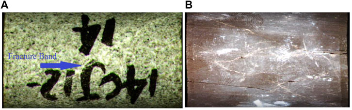
FIGURE 1. Core photos after triaxial fracturing. (A) A post-frac sandstone. The fractures are barely opened and distributed in the form of faint bands. (B) A post-frac shale. Some fractures are filled with fragmental products, appearing white. The unfilled fractures are black.
In this study, we propose a set of experimental methods, including core sample fracturing, image acquisition, and fracture analysis, to quantitatively analyze fracture complexity. We attempt to keep the fractured rocks not scattered by controlling a constant strain rate during the triaxial compression. In addition, we summarize a set of fracture grading methods for cylindrical samples after triaxial fracturing. Subsequently, we can conveniently extract the characteristic parameters of each fracture, such as fracture length, width, and dip angle. Based on the extracted parameters, we propose a calculation method for the fracture complexity after triaxial fracturing treatment.
In this research study, we select 24 gray–black mud shale samples drilled from Longmaxi and Wufeng formations in the Zhaotong area of the Sichuan Basin. All drilled samples are cut in the direction parallel to the bedding planes and machined to cylinders with a diameter of 2.54 cm and a length ranging from 4.5 to 5.0 cm. Figure 2 shows the results of the X-ray diffraction (XRD) analysis, which indicate that the quartz content ranges from 13.9% to 59.9%, the feldspar content ranges from 1.6% to 10.9%, the carbonate mineral (e.g., calcite, dolomite, and ferrodolomite) content ranges from 8.4% to 60.9%, and the clay content ranges from 8.2% to 44.1%. Figure 3 shows the scanning electron microscope (SEM) images for #15 sample at two different scales. The fractures are relatively developed in the direction parallel to the bedding plane. The clay minerals display a sheet-like structure and are distributed in directional orientation sub-parallel to the bedding plane.
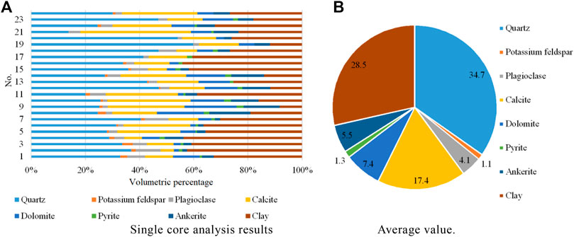
FIGURE 2. X-ray diffraction (XRD) analysis results for 24 shale samples. (A) Single-core analysis results. (B) Average value.
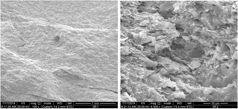
FIGURE 3. Scanning electron microscope (SEM) images for #15 sample.
We carry out the triaxial tests on all 24 samples using a servo-hydraulically controlled triaxial testing system, AutoLab 1,500 manufactured by New England Research Inc., as shown in Figure 4A. The triaxial testing system comprises a load cell, pressure intensifier that allows applying the confining pressure up to 68 MPa, pore pressure system, and digital recording system. The sample, wrapped with a Viton rubber, is placed between the top and bottom endcaps, as shown in Figure 4B. The contacting area between the buffer and sample is twined by copper wires to ensure good alignment and avoid potential sliding during the measurements. The axial strain (εa) is recorded by mounting a pair of linear variable differential transformers (LVDTs) between the top and bottom endcaps. The radial strain (εr) is measured by placing another LVDT at the middle of the sample. The precision of strain measurements is about 0.01 μm. Given that the selected shales have visible bedding planes in the direction of axial loading, the radial LVDT is fixed in the direction perpendicular to the bedding plane.
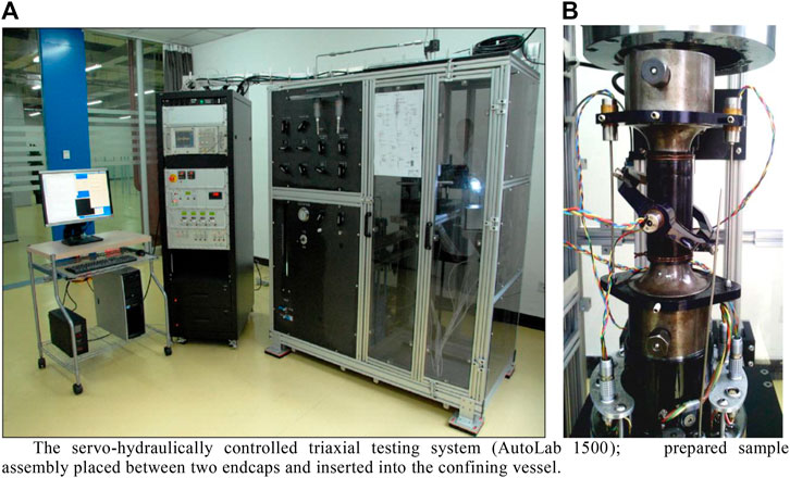
FIGURE 4. Triaxial testing system and prepared sample. (A) Servo-hydraulically controlled triaxial testing system (AutoLab 1500); (B) prepared sample assembly placed between two endcaps and inserted into the confining vessel.
In this study, the main equipment used for collecting core images after triaxial compression is the JB-PDC core optical image scanner developed by Huafu Company (Figure 5). The equipment mainly comprises a camera and sample carrier. The camera is a line-array camera with a resolution of 2000 dpi. The sample carrier is capable of loading samples with a flat surface or a sample tray with flat particles. The sample carrier can be driven to scan the sample horizontally. It can also load a cylindrical sample, which drives the sample to roll in situ under the camera by the rotation of two rollers. Figure 5 shows that the side surface of a cylindrical sample is unfolded into a rectangular image after rolling the sample in the scanner. The rectangular image can be restored to a cylindrical shape, as shown in Figures 1, 2.
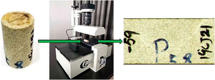
FIGURE 5. JB-PDC core optical image scanner and its principle.
The experimental procedures for quantitatively analyzing the fracture complexity after triaxial fracturing treatment of 24 shale samples include five steps:
1) Carrying out triaxial fracturing experiments to achieve a state of “fractured without scattering”;
2) Scanning the core images after triaxial fracturing treatment and acquiring the fracture information;
3) Preprocessing the core images and conducting fracture classification;
4) Extracting the fracture parameters, such as length, width, and dip angle;
5) Calculating the surface fracture rate and fracture dip dispersion. Subsequently, calculating the fracture complexity.
The sample assemblage is mounted inside the confining vessel. The vessel is, subsequently, filled with mineral oil by driving the confining pump. Then, we move the hydraulic piston downward to touch the top endcap and apply axial stress on the rock sample. To ensure the comparability of the fracture complexity of 24 shale samples, a uniform fracturing degree must be controlled during the measurements. First, the confining pressure is set to a value simulating the in situ horizontal effective stress at the original buried depth. Second, the axial loading is controlled with a constant strain rate, that is, lowering the hydraulic piston at a constant speed to avoid squashing the cores. After fracturing, the hydraulic piston slowly lowers with a constant speed, and the axial stress is released automatically. Thus, we can monitor the stress–strain evolution to determine the fracturing degree.
A large number of experimental observations have revealed that the fracture would develop with different stages under conditions of controlling a constant strain rate. Figure 6 shows the applied stress as a function of time in the process of triaxial fracturing for a shale sample. When the hydraulic piston lowers downward, the axial stress increases and the stress inside the rock accumulates. When the axial stress is beyond point A, the internal microstructure inside the rock starts getting destroyed. When the axial stress reaches the compressive strength, point B, the microstructural fractures accumulate to form a macro-fracture, and the axial stress quickly decreases. With the macro-fracture extension, the internal stress quickly releases. The stress release rate is greater than the stress increase rate caused by lowering the hydraulic piston. The first-level fracture extension would stop when the fracture front stress is lower than the residual strength of the rock. Subsequently, the axial stress begins to accumulate again. Therefore, we can observe point C in the stress–time curve. As the hydraulic piston continues to be lowered, the stress accumulation inside the rock continues. When the first-level residual strength (point D) is reached, the internal structure of the rock is destroyed again, accompanied by fracture extension or newborn fractures. The stress is released again and decreases by showing the second-level residual strength (point E). With such periodical processes, the rock sample is shattered completely. The segment from points C to D represents the development of the first-level fractures. To ensure similar fracturing degree for all 24 samples, we uniformly compress all samples to point D.
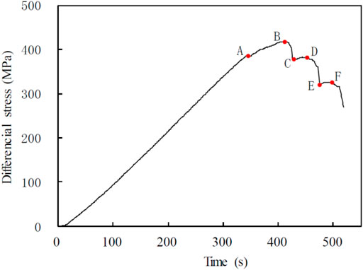
FIGURE 6. Differential stress and strain vs. time in triaxial fracturing.
As shown in Figure 5, the post-fractured sample is placed on the JB-PDC core optical image scanner. The fractures on the side surface of the cylindrical sample are displayed on a planar graph. For a cylindrical sample with a diameter of 1.0 inch, the resolution of the scanner is about 0.04 mm.
Even if the triaxial fracturing experiment described in Section 2.3.1 is used to control the degree of fracturing, most of the post-fractured images are still difficult to be identified due to the low fracture opening degree, background interference, and insufficient acquisition accuracy. It is necessary to preprocess the core images to make the fractures recognizable. Although the traditional image processing software has poor results in brightness, contrast, and other color difference processing, it is still easy to be used for observing the fractures in actual core samples. We summarize a set of fracture classification methods by analyzing the core fracturing process and observing the post-fractured core images. The fracture images are preprocessed accordingly to make the fractures easy to be identified and extracted.
The fracture classification method is summarized in Table 1. The fractures are classified into four levels according to the fracture morphology (extension degree, penetration degree, width, and dip angle of each fracture) and fracture generation mechanism.
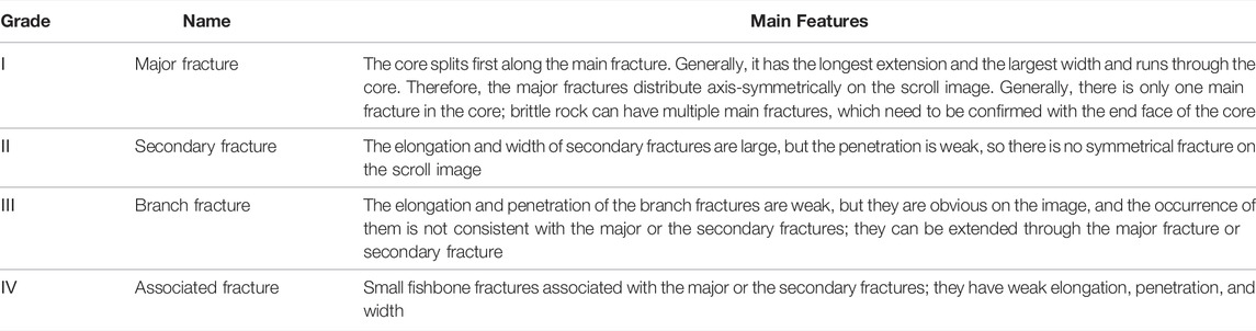
TABLE 1. Post-fractured core fracture classification method.
According to the aforementioned classification method, the fractures with different levels are redrawn with lines of different thicknesses, as shown in Figure 7. In Figure 7A, the original core image after fracturing has a low fracture opening degree and is highly affected by the artificial markers. In Figure 7B, through the image preprocessing in Section 2.3.3, the fractures after triaxial compression are clearly identified.
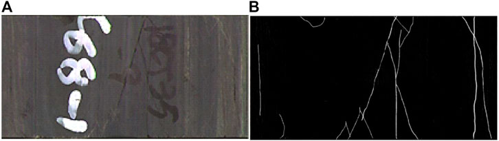
FIGURE 7. (A) An original post-frac core image. Fractures are difficult to be identified due to the image resolution. (B) A post-frac core image preprocessed with the method in Section 2.3.3. The fractures are clearly identified.
We extract the length of each fracture and the height and width pixel values of the circumscribed rectangle. The length is subsequently converted into the actual length:
where li is the actual length of the ith fracture (mm), lp is the fracture’s pixel length (pixel), h is the actual height of the sample (mm), and hp is the sample’s pixel height (pixel). The fracture width is the product of each pixel length and the corresponding pixel value.
The dip angle of each fracture can be calculated with the height and width of the circumscribed rectangle:
where A is the fracture dip angle (degree), ranging between 0° and 90°; and H and W are the height and width of the circumscribed rectangle (pixel), respectively.
The complex fracture network after triaxial fracturing treatment has three characteristics: large number, large fracture, and complex morphology. Therefore, the fracture complexity is a function of the number, size, and morphology of the fractures. The fracture number can be directly counted from the fracture image. The fracture size can be characterized by the fracture area in the image. The more discrete the fracture dip angle after core compression, the closer the fracture is to a network. As a result, the fracture morphology can be characterized by the disorder degree of the fracture dip angle. We propose the concepts of surface fracture rate and fracture dip dispersion.
The surface fracture rate is the area sum of all fractures divided by the sum of the side surfaces.
where Rf is the surface fracture rate (dimensionless), Si is the area of the ith fracture (mm2), and Sl is the area of the side surface (mm2).
The fracture dip dispersion is calculated by Eq. (6).
where Da is the fracture dip dispersion (dimensionless),
The surface fracture rate and fracture dip dispersion contain information of the number, size, and morphology of the generated fractures. According to the statistical analysis method, the surface fracture rate and fracture dip dispersion are averaged to represent the fracture complexity (Fc). The surface fracture rate and fracture dip dispersion are necessary to be normalized because the values in different samples are quite different.
where Fc is the fracture complexity. According to the theoretical and empirical analyses of cylindrical samples with a diameter of 1 inch, the maximum and minimum surface fracture rates are 3 and 0, respectively. The maximum and minimum fracture dip dispersion is 45° and 0°, respectively. Hence, Eq. 7 can be simplified as follows:
The 24 core samples were subjected to triaxial fracturing according to the method described in Section 2.3.1. After fracturing, the samples remained cylindrical (partially split into two halves and bonded with glue), and then optical scroll scanning was performed according to the method described in Section 2.3.2. Figure 8 shows the photos of the post-fractured cores arranged by sample number.
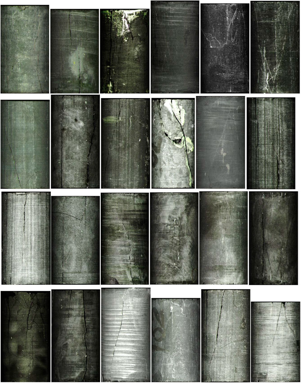
FIGURE 8. Photos of 24 post-fractured core samples.
Figure 9 is a group photo of the unfolded side surface of the 24 cores (sorted by NO.), preprocessed according to the method described in Section 2.3.3, and the parameters of each fracture were extracted according to the method described in Section 2.3.4. Then, the fracture rate (
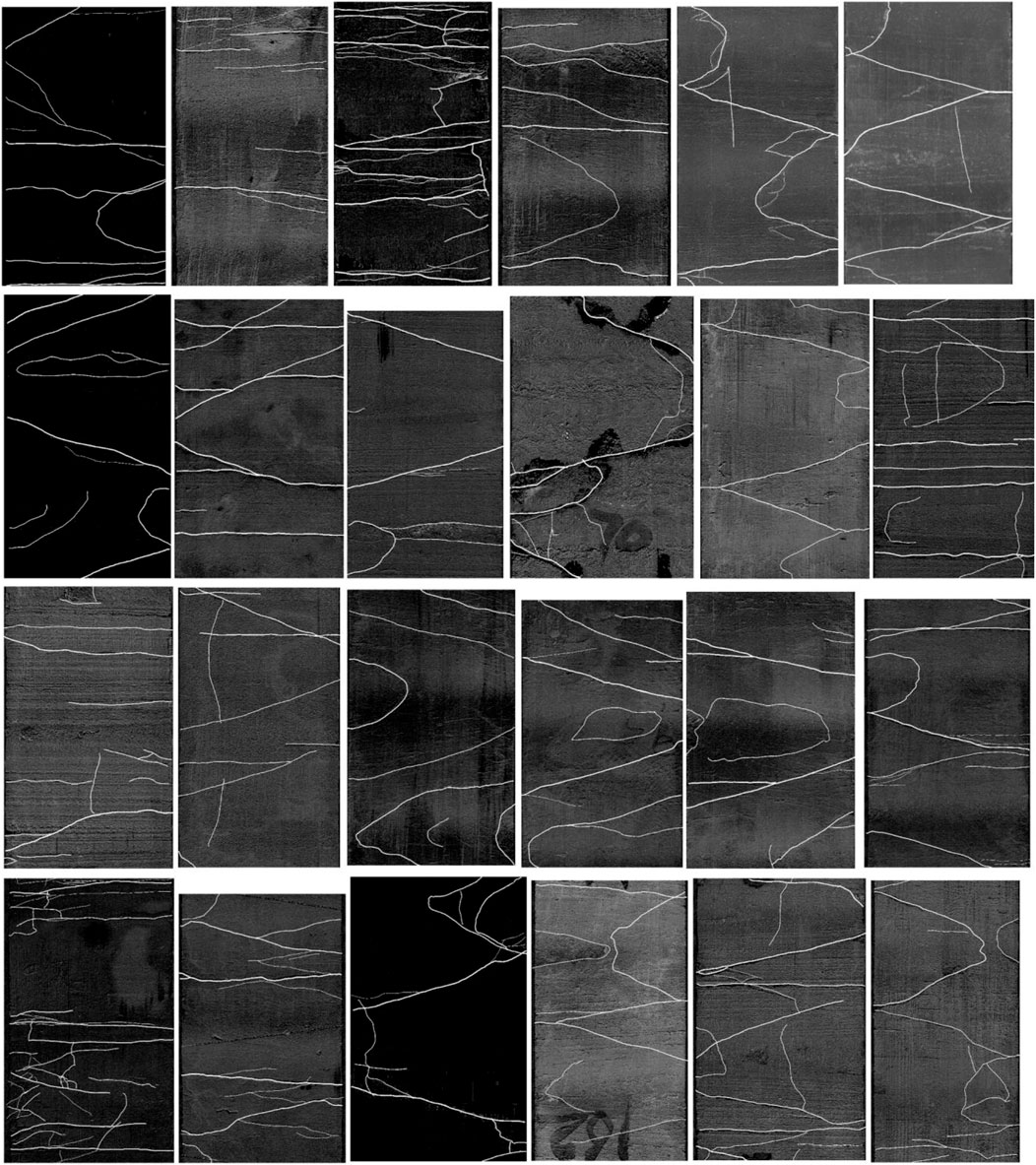
FIGURE 9. Crack extraction results of the lateral surface expansion map of 24 cores after compression test.
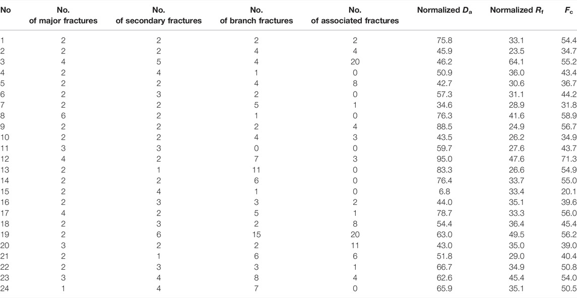
TABLE 2. Fracturing and fracture analysis results of 24 cores after compression test.
The fractal theory was proposed by Mandelbrot (1967). It is one of the important branches of modern nonlinear science and is widely used in many fields such as mathematics, physics, chemistry, biology, medicine, geography, and geology. Xie (1992) first combined the fractal theory with rock mechanics and studied the relationship between fracture fractals and mechanical properties of fracture structure planes. Later, numerous researchers studied the relationship between a large number of fractures and fractal dimensions and achieved good results. At present, the commonly used fractal description methods for rock fractures include the area perimeter method (Miller and Ross, 1993), box dimension method (Peng et al., 2004), and variogram method. The box dimension method is widely used due to operation convenience. The box dimension method uses the fracture fractal dimension to characterize the irregularity of fractures.
In this study, after preprocessing the core images of 24 shales, the box dimension method is used to calculate the fractal dimension. The square grid with a length of r is used to cover the entire core. The number of square grids [N(r)] containing the fractures is counted. The side length of the square grid (r) is gradually changed to obtain N(r). In the double-logarithmic coordinate system, the least square is used to make regression analysis on the statistical data (r and N(r)). The slope of the regression line is the fractal dimension (D). The calculation results are shown in Table 2. The parameters in Tables 1, 2 are cross-plotted, as shown in Figure 10. The fractal dimension is positively correlated with fracture complexity, but the correlation is weak. The fractal dimension does not show correlation with the fracture dip dispersion, but has a good linear correlation with the surface fracture rate. This is because the fractal dimension only considers the proportion of abnormal points in the binarized image, which is essentially the same as the surface fracture rate. However, the image noise has an effect on the fractal dimension but has no effect on the surface fracture rate. Therefore, in contrast, it is more advantageous in describing the complex fractures after triaxial fracturing treatment by using the fracture complexity than by using the fractal dimension.
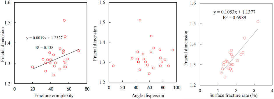
FIGURE 10. Relationship between the fractal dimension and fracture complexity, angle dispersion, and surface fracture rate.
Table 3 shows the rock mechanical parameters for all 24 shale samples. We use Eq. 1 to calculate the brittleness index (BI-Mi). According to the ultrasonic velocity data, we calculate the dynamic Young’s modulus and Poisson’s ratio, which are subsequently used to calculate the brittleness index (BI-Ac), according to Eq. 2. The maximum and minimum values of Young’s modulus and Poisson’s ratio are from the empirical values of the target reservoirs, which are 70.2 GPa and 40.0 GPa and 0.33 and 0.04, respectively. The static Young’s modulus and Poisson’s ratio obtained in the triaxial fracturing experiment are used to calculate the rock mechanical brittleness index (BI-Me), according to Eq. 2. Figure 11 shows the comparisons of brittleness index from three methods. The fracture complexity (Fc) and brittleness index (BI-Mi) show a positive correlation. There is no obvious correlation between Fc and BI-Ac or BI-Me.
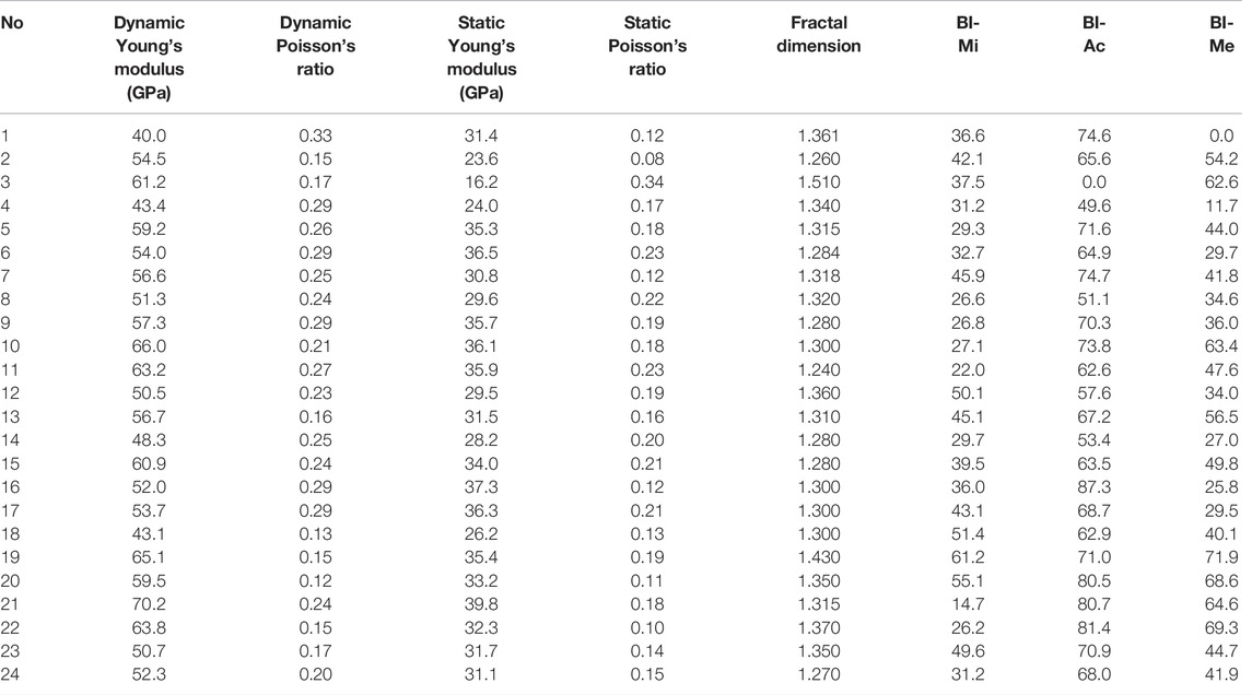
TABLE 3. Calculated brittleness indices.
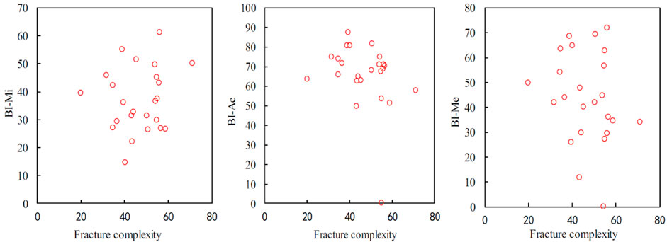
FIGURE 11. Relationship between the brittleness index and fracture complexity.
Figure 12 shows the correlations between mineral contents and fracture complexity. The fracture complexity has a positive correlation with the quartz, calcite, and dolomite content. The fracture complexity has a negative correlation with clay content. The fracture complexity has no obvious relationship with feldspar content.
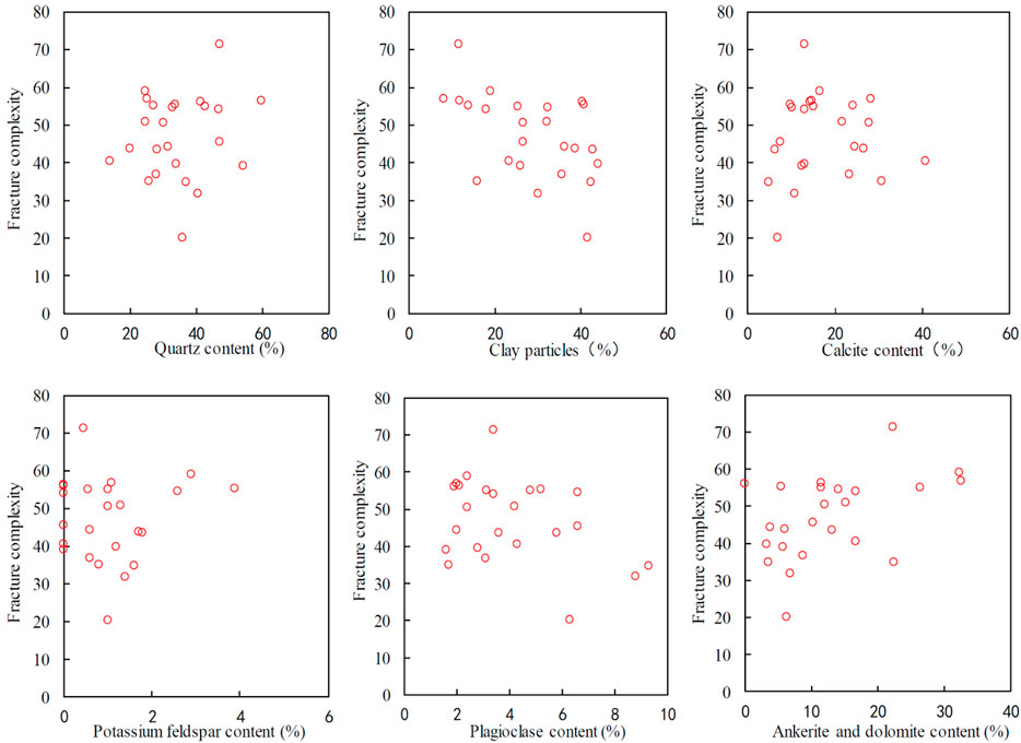
FIGURE 12. Relationship between mineral content and fracture complexity.
In this study, the cores are broken by the axial compression method, which would finally result in shear fracturing. In practice, reservoirs are broken by increasing the pore pressure in hydraulic fracturing, which would result in tensile fracturing. Although the fracturing methods are different, due to the microscopic heterogeneity and anisotropy of the rock, the fractures of the two fracturing methods are preferentially generated or extended along the weak planes of the internal microstructure. The number and morphology of fractures and the fracturing strength are all determined by the weak planes at micro scale. Therefore, the rock mechanical properties obtained from the triaxial compression experiment can be applied to hydraulic fracturing to analyze the fracability of oil and gas reservoirs (Jin et al., 2015; Li N. et al., 2018).
The quantification of the fracture complexity proposed in this study is a new technology. Many new problems have risen in practical applications and are still being improved. For example, the verticality and flatness of the cylindrical core end face has a serious impact on fracture morphology, which puts forward higher requirements for core processing accuracy than the current industry level. The Fc calculation method is still being optimized. For example, the calculation of fracture dip dispersion in Eq. (4) does not consider the influence of fracture size. In addition, the image preprocessing software is being developed to formulate rules to realize automatic fracture classification and reduce the artificial influences. The microscopic mechanism that affects the surface fracture rate and fracture dip dispersion also needs to be studied.
The post-fracturing fracture complexity describes the complexity of the primary fractures generated after core fracturing. A larger Fc represents a better fracturing result but it does not fully represent the fracability of the rock. To fully analyze the fracability of rocks, the fracturing process can be divided into three stages: In the first stage, the internal microstructures are continuously destroyed until the axial stress increases to the compressive strength. In the second stage, the microscopic fractures are connected to form macroscopic fractures, and the strength of the rock decreases. In the third stage, the macroscopic fractures continue to extend along the weak planes, and the energy of fracturing is also reduced until it is insufficient to support the fracture extension. Through the aforementioned analysis, in addition to the fracture complexity, a complete description of the fracturing process requires rock strength and fracture extensibility. Less rock strength means that a smaller stress is required for hydraulic fracturing. Therefore, the rock strength and fracability are negatively correlated. In addition, a faster fracture extension after fracturing means a faster hydraulic fracturing speed, resulting in less proppant, shorter soaking time, and lower cost. Therefore, the fracture extensibility is positively related to the fracability. For the triaxial fracturing experiment in this study, the strength can be described by the triaxial compressive strength, and the extensibility of the fracture produced after compression can be described by the analysis of the stress–strain curve. Through the triaxial fracturing experiment, the rock fracability can be completely analyzed.
We propose a set of methods for quantitatively analyzing the fracture complexity of rocks after triaxial fracturing. The results suggest that
1) Fracture complexity can represent the complex fracture characteristics of mud shales after triaxial fracturing;
2) The fractal dimension of fractures has a good linear correlation with the surface fracture rate and has no correlation with the fracture dip dispersion. By comparison, the fracture complexity is more suitable for describing the complex fracture network than the fractal dimension;
3) Fracture complexity has no obvious relationship with the brittleness index based on Young’s modulus and Poisson’s ratio and has a positive correlation with the brittleness index based on mineral compositions;
4) Fracture complexity is positively correlated with the content of quartz, calcite, and dolomite and negatively correlated with the content of clay minerals and has no obvious relationship with the content of feldspar.
The quantitative analysis method for the fracture complexity calculation after triaxial fracturing is a new technology. There are still many problems to be solved. However, this technology provides a solution to the bottleneck problem in the fracturing evaluation of unconventional oil and gas reservoirs and has good application prospects.
The original contributions presented in the study are included in the article/Supplementary Material, further inquiries can be directed to the corresponding author.
All authors listed have made a substantial, direct, and intellectual contribution to the work and approved it for publication.
This work is supported by the Scientific Research and Technology Development Project of the China National Petroleum Corporation (2021DJ4003).
YZ and XL were employed by the CNPC Logging Company Limited. Author YW was employed by the SINOPEC Geophysical Research Institute.
The remaining authors declare that the research was conducted in the absence of any commercial or financial relationships that could be constructed as a potential conflict of interest.
All claims expressed in this article are solely those of the authors and do not necessarily represent those of their affiliated organizations, or those of the publisher, the editors, and the reviewers. Any product that may be evaluated in this article, or claim that may be made by its manufacturer, is not guaranteed or endorsed by the publisher.
Ai, C., Zhang, J., Li, Y., Zeng, J., Yang, X., and Wang, J. (2016). Estimation Criteria for Rock Brittleness Based on Energy Analysis during the Rupturing Process. Rock Mech. Rock Eng. 49 (12), 4681–4698. doi:10.1007/s00603-016-1078-x
Akinbinu, V. A. (2017). Relationship of Brittleness and Fragmentation in Brittle Compression. Eng. Geology. 221, 82–90. doi:10.1016/j.enggeo.2017.02.029
Bai, M. (2016). Why Are Brittleness and Fracability Not Equivalent in Designing Hydraulic Fracturing in Tight Shale Gas Reservoirs. Petroleum 2 (1), 1–19. doi:10.1016/j.petlm.2016.01.001
Barree, R. D. D., Cox, S. A. A., Miskimins, J. L. L., Gilbert, J. V. V., and Conway, M. W. W. (2015). Economic Optimization of Horizontal-Well Completions in Unconventional Reservoirs. SPE Prod. Operations 30 (04), 293–311. doi:10.2118/168612-pa
Brace, W. F., Paulding Jr., B. W., and Scholz, C. (1966). Dilatancy in the Fracture of Crystalline Rocks. J. Geophys. Res. 71 (16), 3939–3953. doi:10.1029/jz071i016p03939
Feng, R., Zhang, Y., Rezagholilou, A., Roshan, H., and Sarmadivaleh, M. (2020). Brittleness Index: From Conventional to Hydraulic Fracturing Energy Model. Rock Mech. Rock Eng. 53 (2), 739–753. doi:10.1007/s00603-019-01942-1
Guo, T., Zhang, S., Qu, Z., Zhou, T., Xiao, Y., and Gao, J. (2014). Experimental Study of Hydraulic Fracturing for Shale by Stimulated Reservoir Volume. Fuel 128, 373–380. doi:10.1016/j.fuel.2014.03.029
Holt, R. M., Fjær, E., Stenebråten, J. F., and Nes, O.-M. (2015). Brittleness of Shales: Relevance to Borehole Collapse and Hydraulic Fracturing. J. Pet. Sci. Eng. 131, 200–209. doi:10.1016/j.petrol.2015.04.006
Ishii, E., Sanada, H., Funaki, H., Sugita, Y., and Kurikami, H. (2011). The Relationships Among Brittleness, Deformation Behavior, and Transport Properties in Mudstones: An Example from the Horonobe Underground Research Laboratory, Japan. J. Geophys. Res. Solid Earth 116 (B9), 1–15. doi:10.1029/2011jb008279
Iyare, U. C., Blake, O. O., and Ramsook, R. (2021). Brittleness Evaluation of Naparima Hill Mudstones. J. Pet. Sci. Eng. 196, 107737. doi:10.1016/j.petrol.2020.107737
Jaeger, J. C., Cook, N. G., and Zimmerman, R. (1969). Fundamentals of Rock Mechanics. London: Methuen.
Jarvie, D. M., Hill, R. J., Ruble, T. E., and Pollastro, R. M. (2007). Unconventional Shale-Gas Systems: The Mississippian Barnett Shale of North-Central Texas as One Model for Thermogenic Shale-Gas Assessment. AAPG Bull. 91 (4), 475–499. doi:10.1306/12190606068
Jin, X., Shah, S. N., Roegiers, J.-C., and Zhang, B. (2015). An Integrated Petrophysics and Geomechanics Approach for Fracability Evaluation in Shale Reservoirs. SPE J. 20 (03), 518–526. doi:10.2118/168589-pa
Li, J., Li, Y., and Wu, K. (2021). “An Efficient Higher Order Displacement Discontinuity Method with Joint Element for Hydraulic Fracture Modeling,” in 55th US Rock Mechanics/Geomechanics Symposium (OnePetro, Virtual, June 2021).
Li, J., Yu, W., Guerra, D., and Wu, K. (2018). Modeling Wettability Alteration Effect on Well Performance in Permian basin with Complex Fracture Networks. Fuel 224, 740–751. doi:10.1016/j.fuel.2018.03.059
Li, N., Zhang, S., Zou, Y., Ma, X., Wu, S., and Zou, Y. (2018). Experimental Analysis of Hydraulic Fracture Growth and Acoustic Emission Response in a Layered Formation. Rock Mech. Rock Eng. 51 (4), 1047–1062. doi:10.1007/s00603-018-1547-5
Li, X., Wang, S., Ge, S., Reza, M., and Li, Z. (2018). Investigation on the Influence Mechanism of Rock Brittleness on Rock Fragmentation and Cutting Performance by Discrete Element Method. Measurement 113, 120–130. doi:10.1016/j.measurement.2017.07.043
Li, Y., Long, M., Tang, J., Chen, M., and Fu, X. (2020). A Hydraulic Fracture Height Mathematical Model Considering the Influence of Plastic Region at Fracture Tip. Pet. Exploration Develop. 47 (1), 184–195. doi:10.1016/S1876-3804(20)60017-9
Li, Y., Jia, D., Rui, Z., Peng, J., Fu, C., and Zhang, J. (2017). Evaluation Method of Rock Brittleness Based on Statistical Constitutive Relations for Rock Damage. J. Pet. Sci. Eng. 153, 123–132. doi:10.1016/j.petrol.2017.03.041
Li, Y., Long, M., Zuo, L., Li, W., and Zhao, W. (2019). Brittleness Evaluation of Coal Based on Statistical Damage and Energy Evolution Theory. J. Pet. Sci. Eng. 172, 753–763. doi:10.1016/j.petrol.2018.08.069
Ma, X., Li, N., Yin, C., Li, Y., Zou, Y., Wu, S., et al. (2017). Hydraulic Fracture Propagation Geometry and Acoustic Emission Interpretation: A Case Study of Silurian Longmaxi Formation Shale in Sichuan Basin, SW China. Pet. Exploration Develop. 44 (6), 1030–1037. doi:10.1016/s1876-3804(17)30116-7
Mandelbrot, B. (1967). How Long Is the Coast of Britain? Statistical Self-Similarity and Fractional Dimension. Science 156 (3775), 636–638. doi:10.1126/science.156.3775.636
Miller, K. S., and Ross, B. (1993). An Introduction to the Fractional Calculus and Fractional Differential Equations. New York: Wiley.
Nejati, H. R., and Ghazvinian, A. (2014). Brittleness Effect on Rock Fatigue Damage Evolution. Rock Mech. Rock Eng. 47 (5), 1839–1848. doi:10.1007/s00603-013-0486-4
Peng, R. D., Xie, H. P., and Ju, Y. (2004). Computation Method of Fractal Dimension for 2-D Digital Image. J. China Univ. Mining Technol. 33 (1), 19–24. doi:10.1023/B:APIN.0000033637.51909.04
Qin, H., and Yang, X. (2019). Log Interpretation Methods for Measuring the Brittleness of Tight Reservoir. Well Logging Technol. 43 (5), 509–513+530. doi:10.16489/j.issn.1004-1338.2019.05.013
Rickman, R., Mullen, M. J., Petre, J. E., Grieser, W. V., and Kundert, D. (2008). “A Practical Use of Shale Petrophysics for Stimulation Design Optimization: All Shale Plays Are Not Clones of the Barnett Shale,” in SPE annual technical conference and exhibition (Denver, Colorado, USA, September 2008: Society of Petroleum Engineers). doi:10.2118/115258-ms
Stanchits, S., Burghardt, J., and Surdi, A. (2015). Hydraulic Fracturing of Heterogeneous Rock Monitored by Acoustic Emission. Rock Mech. Rock Eng. 48 (6), 2513–2527. doi:10.1007/s00603-015-0848-1
Tarasov, B., and Potvin, Y. (2013). Universal Criteria for Rock Brittleness Estimation under Triaxial Compression. Int. J. Rock Mech. Mining Sci. 59, 57–69. doi:10.1016/j.ijrmms.2012.12.011
Vernik, L. (2016). Seismic Petrophysics in Quantitative Interpretation. Society of Exploration Geophysicists, Tulsa. doi:10.1190/1.9781560803256
Wang, Y., Li, H., Mitra, A., Han, D.-H., and Long, T. (2020). Anisotropic Strength and Failure Behaviors of Transversely Isotropic Shales: An Experimental Investigation. Interpretation 8 (3), SL59–SL70. doi:10.1190/INT-2019-0275.1
Wang, Y., Zhao, L., Han, D.-H., Mitra, A., Li, H., and Aldin, S. (2021). Anisotropic Dynamic and Static Mechanical Properties of Organic-Rich Shale: The Influence of Stress. Geophysics 86 (2), C51–C63. doi:10.1190/geo2020-0010.1
Wen, T., Tang, H., and Wang, Y. (2020). Brittleness Evaluation Based on the Energy Evolution throughout the Failure Process of Rocks. J. Pet. Sci. Eng. 194, 107361. doi:10.1016/j.petrol.2020.107361
Xie, H. (1992). Fractal Geometry and its Application in Rock and Soil Mechanics. Chin. J. Geotechnical Eng. 14 (1), 14–24.
Zhang, D., Ranjith, P. G., and Perera, M. S. A. (2016). The Brittleness Indices Used in Rock Mechanics and Their Application in Shale Hydraulic Fracturing: A Review. J. Pet. Sci. Eng. 143, 158–170. doi:10.1016/j.petrol.2016.02.011
Zhang, J., Li, Y., Pan, Y., Wang, X., Yan, M., Shi, X., et al. (2021). Experiments and Analysis on the Influence of Multiple Closed Cemented Natural Fractures on Hydraulic Fracture Propagation in a Tight sandstone Reservoir. Eng. Geology. 281, 105981. doi:10.1016/j.enggeo.2020.105981
Zhang, S., Guo, T., Zhou, T., Zou, Y., and Mu, S. (2014). Fracture Propagation Mechanism experiment of Hydraulic Fracturing in Natural Shale. Acta Petrolei Sinica 35 (3), 496–503. doi:10.7623/syxb201403011
Keywords: triaxial compression, fracability, fracture morphology, fractal dimension, fracture complexity
Citation: Zhang Y, Ma J, Wang Y, Wang F, Li X and Zhao L (2022) Quantification of the Fracture Complexity of Shale Cores After Triaxial Fracturing. Front. Earth Sci. 10:863773. doi: 10.3389/feart.2022.863773
Received: 27 January 2022; Accepted: 08 March 2022;
Published: 01 April 2022.
Edited by:
Yuwei Li, Liaoning University, ChinaReviewed by:
Junxin Guo, Southern University of Science and Technology, ChinaCopyright © 2022 Zhang, Ma, Wang, Wang, Li and Zhao. This is an open-access article distributed under the terms of the Creative Commons Attribution License (CC BY). The use, distribution or reproduction in other forums is permitted, provided the original author(s) and the copyright owner(s) are credited and that the original publication in this journal is cited, in accordance with accepted academic practice. No use, distribution or reproduction is permitted which does not comply with these terms.
*Correspondence: Yang Wang, eXdhbmcwNjA1QGhvdG1haWwuY29t, b3JjaWQub3JnLzAwMDAtMDAwMi01NzkyLTk4NTI=
†These authors have contributed equally to this work and share first authorship
Disclaimer: All claims expressed in this article are solely those of the authors and do not necessarily represent those of their affiliated organizations, or those of the publisher, the editors and the reviewers. Any product that may be evaluated in this article or claim that may be made by its manufacturer is not guaranteed or endorsed by the publisher.
Research integrity at Frontiers
Learn more about the work of our research integrity team to safeguard the quality of each article we publish.